Sequential Monte Carlo methods for epidemic data

(1)

Sequential Monte Carlo Methods

for Epidemic Data

Jessica Welding

Department of Mathematics and Statistics

Submitted for the degree of Doctor of Philosophy at

Lancaster University

(2)

Sequential Monte Carlo Methods for Epidemic Data Jessica Welding

Submitted for the degree of Doctor of Philosophy at Lancaster University January 2020

Abstract

Epidemics often occur rapidly, with new cases being observed daily. Due to the frequently severe social and economic consequences of an outbreak, this is an area of research that benefits greatly from online inference. This motivates research into the construction of fast, adaptive methods for performing real-time statistical analysis of epidemic data.

The aim of this thesis is to develop sequential Monte Carlo (SMC) methods for infec-tious disease outbreaks. These methods utilize the observed removal times of individuals, obtained throughout the outbreak. The SMC algorithm adaptively generates samples from the evolving posterior distribution, allowing for the real-time estimation of the parameters underpinning the outbreak. This is achieved by transforming the samples when new data arrives, so that they represent samples from the posterior distribution which incorporates all of the data.

To assess the performance of the SMC algorithm we additionally develop a novel Markov chain Monte Carlo (MCMC) algorithm, utilising adaptive proposal schemes to improve its mixing. We test the SMC and MCMC algorithms on various simulated outbreaks, finding that the two methods produce comparable results in terms of param-eter estimation and disease dynamics. However, due to the parallel nature of the SMC algorithm it is computationally much faster.

The SMC and MCMC algorithms are applied to the 2001 UK Foot-and-Mouth out-break: notable for its rapid spread and requirement of control measures to contain the outbreak. This presents an ideal candidate for real-time analysis. We find good agree-ment between the two methods, with the SMC algorithm again much quicker than the MCMC algorithm. Additionally, the performed inference matches well with previous work conducted on this data set.

Overall, we find that the SMC algorithm developed is suitable for the real-time analysis of an epidemic and is highly competitive with the current gold-standard of

(3)

Acknowledgements

First I must credit the financial support offered to me by the EPSRC, which allowed me to complete this work.

I must also thank my eternally optimistic supervisor, Pete Neal, I am truly grateful for your supervision and guidance during my PhD, as well as your seemingly endless patience! I additionally extend my gratitude to Selina Wang, for teaching me to see problems from a different perspective and being an inspiring person to have worked with.

Thanks also to my ever-understanding family and friends, for listening to me moan and understanding when I’m grouchy because everything has broken. Thank you for the cat pictures, the food and cake supplies, for teaching and guiding me to try new things and providing endless (lively!) discussions.

Finally I have to thank my partner David, for being generally a wonderful human being/support team/chef/bug-fixer/bug-catcher/player 2.

(4)

Declaration

I declare that this thesis is my own work and has not been submitted in substantially the same form for the award of a higher degree elsewhere.

(5)

List of Figures

1.1 The target (black) and proposal (orange) density functions. . . 10

1.2 The target and scaled proposal densities. . . 10

1.3 The samples accepted (black) and rejected (orange). . . 10

1.4 A histogram of the accepted samples with the truth overlaid. . . 10

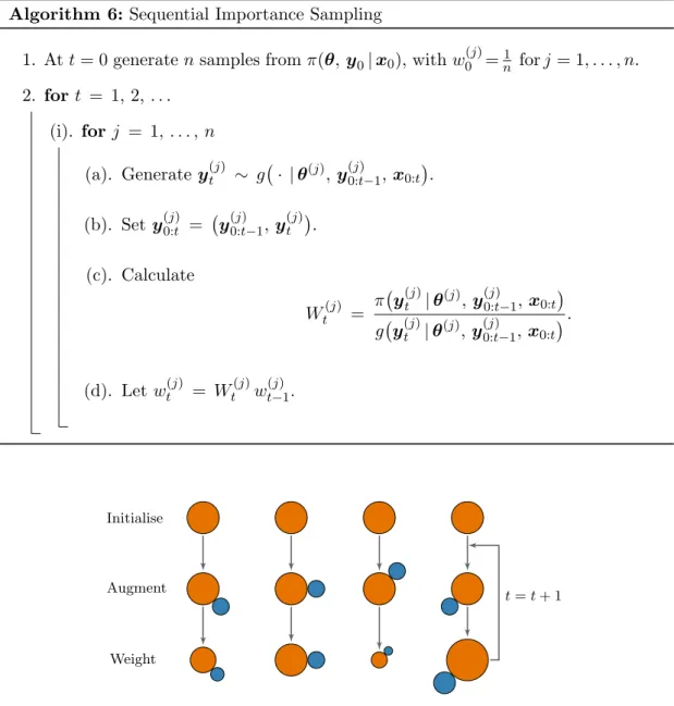
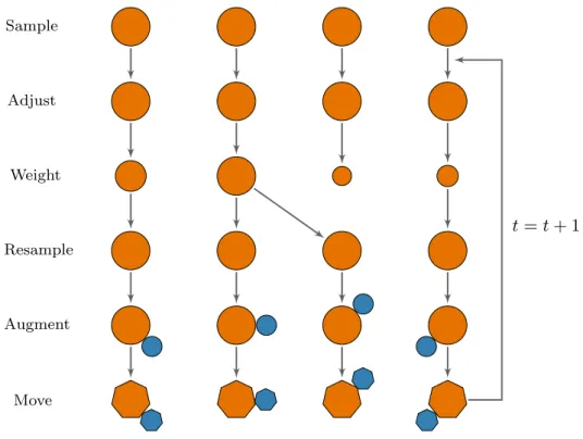
1.5 An illustration of the sequential importance sampling algorithm. The or-ange circles represent the (initial) particles and the blue circles represent the new information sampled during the augmentation step. The size of the particles represents the relative contribution of each particle, depen-dent on their weight. We can see that there is no interaction between the different particles. . . 33

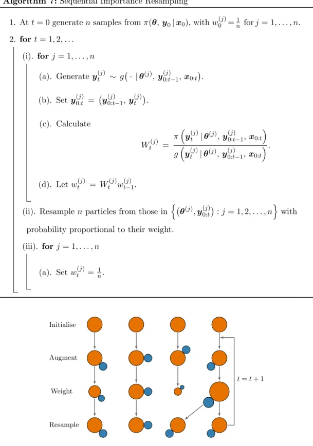
1.6 An illustration of the sequential importance resampling algorithm. . . 36

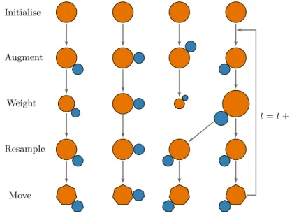
1.7 An illustration of the sequential importance resampling and move algorithm. 39 2.1 The SIR model, often referred to as the ‘general’ model. . . 58

2.2 The SI model, often referred to as the ‘simple’ model. . . 58

2.3 The SEIR model. . . 58

2.4 The SIS model. . . 59

2.5 The SINR model. . . 59

3.1 An illustration of the adjustment process applied to each particle, the cir-cles and squares indicate different individuals. The left-hand side shows the original labelling of the particle and the right-hand side shows a pos-sible amendment, which ensures that the particle is consistent with the new removals observed. . . 108

(12)

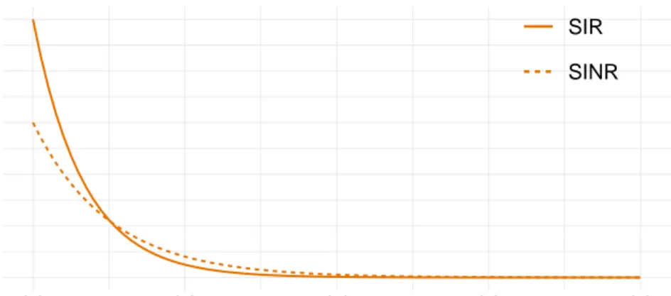
4.1 The transmission probability evaluated for different values of the Eu-clidean distance, d(x, y), for both the SIR outbreak, with γ = 15 and

p= 0.975, and the SINR outbreak, withγ = 10 and p= 0.985. . . 143 4.2 The location of each individual within the population on which the

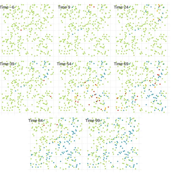
simu-lated SIR outbreak occurs. The colour indicates each individual’s status at the current time step (top-right) as either susceptible (green), infectious (red) or removed (blue). . . 144 4.3 The number of individuals in each of the three states: ‘Susceptible’,

‘In-fectious’, or ‘Removed, at each time step of the SIR outbreak. . . 144 4.4 The location of each individual within the population on which the

simu-lated SINR outbreak occurs. The colour indicates each individual’s status at the current time step (top-left) as either susceptible (green), infectious (red), notified (yellow) or removed (blue). . . 145 4.5 The number of individuals in each of the four states: ‘Susceptible’,

‘Infec-tious’, ‘Notified’, or ‘Removed, at each time step of the SINR outbreak. . . . 145 4.6 Lines showing the median (solid) and the lower (2.5%) and upper (97.5%)

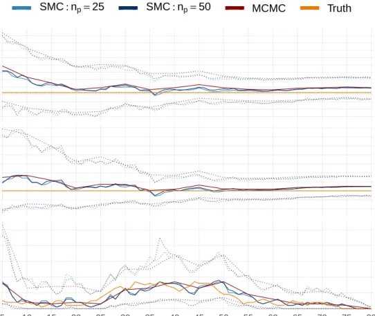
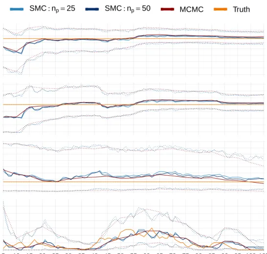
quantiles (dotted) of the samples, at each time step, generated using two runs of the SMC algorithm (blues) and an MCMC algorithm (red), as applied to the SIR outbreak. The SMC algorithm has been applied with movement step of length np = 25 and np = 50. Also shown are the true

values (orange), which were used to simulate the outbreak. The SMC output is shown every time step and the MCMC every 5 times steps (5, 10,. . .). . . 147 4.7 Lines showing the median (solid) and the lower (2.5%) and upper (97.5%)

quantiles (dotted) of the samples, at each time step, generated using two runs of the SMC algorithm (blues) and an MCMC algorithm (red), as applied to the SINR outbreak. The SMC algorithm has been applied with movement step of lengthnp = 25 and np = 50. Also shown are the

true values (orange). The SMC output is shown every time step and the MCMC every 5 times steps (5, 10,. . .). . . 150

(13)

4.8 The density plots generated at the end of the SINR outbreak, using SMC methods (solid blue) applied from the start of the outbreak. We also include the initial particles used to seed the SMC (solid grey) and the prior distributions used (dashed orange). . . 151 4.9 A comparison of the (estimated) time taken to apply both the SMC and

MCMC methods to the SIR and SINR outbreaks, where the former is applied with two values ofnp. The MCMC (black) is run with a burn-in

of b = 10000 and has been applied every 5 time-steps (5, 10, . . .). The SMC has been applied at every time step and split into X jobs, where different values of X are represented by a different colour. . . 155 4.10 A comparison of the particles generated using SMC methods with different

values of np (blues) and MCMC methods (red), as applied to the SINR

outbreak. . . 157 4.11 The average acceptance rates for each proposal step in the MCMC

move-ment step applied to each particle within the SMC algorithm. We consider both the SIR and the SINR simulated outbreaks. . . 159 4.12 The number of unique particles resampled in each iteration of the SMC

algorithm during the resampling step, when different lengths of the move-ment step (np) are considered. . . 160

4.13 A comparison of the output generated using MCMC (red) and SMC meth-ods with np = 25 (blue), where the latter no longer has the particle

ad-justment step. . . 162 4.14 The number of unique particles resampled in each iteration, when using

the SMC algorithm with no adjustment step andnp = 25. The colour of

each bar represents the number of new removals observed at that time step.162 4.15 The mean values (solid) for each parameter generated using the SMC

algorithm which uses either an exponential or a Gaussian distance kernel. Also shown is the mean ±the standard deviation (dashed). . . 164 4.16 The mean values (solid) for each parameter generated using the SMC

algorithm which uses either an exponential or a Gaussian distance kernel. Also shown is the mean ±the standard deviation (dashed). . . 165

(14)

4.17 The transmission probability generated using the mean values outputted using SMC methods (taken at the last day of analysis), under the two different transmission models. Shown in black is the true transmission kernel used to simulate the outbreak. Also shown under each plot is the distribution of the distances between each pair of individuals within the population. . . 166 4.18 The prior distributions we place on the infectious period parameter, a. . . 169 4.19 The density plots of the particles generated for each parameter using

MCMC (solid) and SMC (dashed) methods, compared at two time steps:

t = 45,90. Each colour represents a different prior distribution for pa-rametera. We use a movement step of length np= 50 within the SMC. . 170

4.20 A comparison of the particles generated using the SMC algorithm with both the original, uniform, weighting (U-SMC) and the extension with non-uniform weights (NU-SMC). We additionally show the results from the analogous MCMC algorithm. We compare the samples generated at every 5 times steps. . . 171 4.21 A comparison of the number of unique particles resampled at each

itera-tion of the SMC algorithm, when the two different weighting schemes are used. . . 172 4.22 Illustration of the SMC algorithm for outbreak data, with the addition of

the duplication step. . . 174 4.23 The number of unique particles resampled at each step of an SMC

algo-rithm with movement np = 25 and different values for nd, the number

of duplications. This example is the SIR simulated data considered in Section 4.4. . . 175 4.24 A comparison of the output produced using the SMC algorithm (np =

25), shown every 5 time steps. We have chosen different values for the duplication parameter, nd, where nd = 1 matches the previous analysis

(15)

4.25 A comparison of the time taken to complete each stage of the SMC algo-rithm, as applied to an SIR outbreak, withnp = 25. We have considered

varying levels of duplication, nd = 1,10,20, and different values for the

number of parallel jobs: P = 100,1000. Here the ‘weight’ steps includes both the adjustment and weighting of the particle (see Section 4.5 for further details). . . 176

5.1 Summary of the key events during the 2001 UK Foot-and-Mouth epidemic. The dates are taken from the UK National Audit Office (2002). Note that, as given by UK National Audit Office (2002), the definition of controlled area is “The area affected by general control on movement of susceptible animals”. . . 181 5.2 The farms within Britain that avoided culling (blue) and the farms which

were culled during the 2001 FMD outbreak (red). The large patch of red shows the severity of the outbreak in Cumbria. This is plotted using ArcGIS. . . 182 5.3 The number of new confirmed cases per week, taken from UK National

Audit Office (2002). . . 183 5.4 The total number of farms confirmed as infectious premises, from the time

of the first observed case. . . 188 5.5 The number of notified cases (mN_t ) recorded every 7 days, from timet= 4

up to timet= 32, these will be the times at which we compare the SMC and MCMC methods later in Section 5.6. For comparison, we have also included the state of the outbreak at the time of the first notification,

t= 0. In grey we show every farm and in red we display those confirmed as infectious at timet. . . 189 5.6 The proportion of farms within Cumbria with only cattle, majority cattle

and some sheep, only sheep, majority sheep and some cattle or equal number of cattle and sheep. . . 190 5.7 Histogram of the total number of cattle and sheep on each of the farms

(16)

5.8 The time between notification and removal, for the farms infected within Cumbria during the 2001 UK FMD outbreak. . . 191 5.9 The estimated posterior distribution of each parameter, formed using the

particles generated using SMC (blue) and MCMC (red) methods. In grey we show the initial particles used within the SMC algorithm. . . 200 5.10 The posterior distribution (blue) generated at time t = 32 by the SMC

algorithm with np = 500. Also shown is the prior distribution (orange)

for each parameter. . . 202 5.11 The distance kernel, K(i, j) = exp(−γd(i, j)), evaluated at each of the

values ofγ generated using the three methods, at timest= 11 andt= 32. We only show a portion of the distance range due to the kernel flattening out for very large distances. In black we show the kernel evaluated using the mean value ofγ generated using each method. . . 203 5.12 The probability of infection, qt(i, j), against distance, d(i, j), between

farms of different sizes (see Table 5.3), where ‘Inf’ represents the infectious farm and ‘Sus’ represents the susceptible farm. qt(i, j) is evaluated at the

average value generated for each parameter, at time t = 32, using the three different algorithms. . . 207 5.13 An illustration of the correlation between the parameters, as computed

using the particles generated by the three different algorithms. We display the results for timest= 18 and t= 32. . . 209 5.14 The median number of occults (solid) at each time step, generated using

an SMC algorithm withnp = 500. Also shown are the upper (97.5%) and

lower (2.5%) quantiles represented by the dashed lines. . . 211 5.15 The number of new confirmed cases (notifications) observed at each time

step, from the start of the SMC at t = 4 to the end of the time frame analysed,t= 32. . . 211 5.16 A comparison of the densities generated using the outputs from the MCMC

and SMC methods applied to the FMD data set. The SMC method has been applied using a uniform and a non-uniform adjustment, both with

(17)

5.17 A comparison of the densities generated using the outputs from the MCMC and SMC methods applied to the FMD data set. The SMC method has been applied using a uniform and a non-uniform adjustment, both with

np= 500. . . 214

5.18 The correlation between the particles generated at times t= 18 and t= 32, using MCMC, U-SMC and NU-SMC algorithms, where for the latter two methods np = 200. . . 217

(18)

List of Tables

4.1 The settings used to generate the SIR and the SINR epidemics. The trans-mission parameters areθ= (p, γ, κ), ais the infectious period parameter and dis the length of the notification period in the SINR example. . . 142 4.2 Information relating to the start and end points of when we apply the

SMC algorithm to the SIR and SINR outbreaks. HeremN_t andmR_t denote the number of notified and removed individuals, respectively, at time t. Additionally we denote byT_maxN andT_maxR the time of the last notification and removal, respectively. . . 146 4.3 The prior distributions used within the two simulated outbreaks. . . 147 4.4 A comparison, at three time steps, of the mean and the standard deviation

(S.D.) generated using MCMC and SMC methods on the SIR outbreak, where the latter method has been run with movement steps of length

np= 25 and np = 50. . . 148

4.5 Comparison of the mean and the standard deviation (S.D.) generated using SMC methods, with two values for np, and MCMC methods, as

applied to the SINR outbreak. . . 151 4.6 The settings used to generate the SIR epidemic, for which we aim to

estimate the value of the infectious period distribution parameter,a. . . . 169

5.1 The uninformative priors placed on each parameter used to model the FMD data set. . . 198 5.2 The mean and standard deviation (S.D) of the particles generated for each

parameter, at time stepst= 11,18,25,32. We compare the output from an SMC withnp = 200 andnp= 500, as well as the equivalent MCMC. . 201

(19)

5.3 The composition of the four ‘typical’ farm types in the Cumbria data set, as used in Jewell et al. (2009). . . 206 5.4 The mean and standard deviation generated using the non-uniform SMC

(NU-SMC), with np = 200 and np = 500, and MCMC methods. The

results are displayed at timest= 11,18,25,32. . . 215 5.5 The (maximum) expected time it will take, in hours, to complete the

movement step of the NU-SMC at timet= 32, where we split the calcu-lations intoX parallel jobs and have n= 1000 particles. The burn-in of the comparative MCMC was computed over the course of several days. . . 218

(20)

Chapter 1

Introduction

For many years statisticians have played a pivotal role in furthering the understanding of infectious disease outbreaks (see, for example, Bartlett (1949), Bailey and Thomas (1971), Becker (1979), Gibson (1997), Jewell et al. (2009), Deardon et al. (2010) and Stockdale et al. (2017)). The aim has always remained the same: to gain an understand-ing of the properties which allowed an epidemic to occur, and thus produce strategies for preventing future severe outbreaks.

Epidemics can be an incredibly destructive occurrence: causing the loss of harvests, livestock and often lives. In recent years we have seen many instances of such conse-quences; from the heavy financial burden of the UK Foot-and-Mouth epidemic, estimated at costing over £3 billion to the public sector and over £5 billion to the private sector (UK National Audit Office (2002)), to the devastating loss of life in the recent Ebola outbreak, an estimated 28,616 cases resulting in 11,310 deaths (WHO (2016)). By mod-elling epidemics we can gain vital insight, that is key to understanding and limiting the severity of future outbreaks of infectious diseases.

With the rapid advancement in technology we have gained the ability to collect vast amounts of information about an outbreak. Increasingly this data is extremely rich and often obtained instantaneously, throughout the course of an epidemic. With such data readily available, epidemic modelling has gained the capability to move from retrospective analysis, to real-time analysis. Swiftly obtaining information about the characteristics of an epidemic can then help to inform on control measures that can then be put in place during an active outbreak.

(21)

we aim to illustrate a novel way of utilising advances in computing power to construct a method of inferring the underlying parameters of an infectious disease outbreak, in real time.

1.1 Thesis Structure

This thesis is concerned with the construction of a sequential method of analysing epi-demic data in real time. We will describe the formulation of a generic algorithm, for use in conjunction with epidemic data, and then apply it to both simulated and real data sets.

Chapter 1: Introduction

In this chapter we introduce the Bayesian paradigm and the concept of simulation meth-ods. We then proceed to discuss simple simulation techniques such as inverse, rejection and importance sampling as well as more complex methods such as Markov chain Monte Carlo (MCMC) and sequential Monte Carlo (SMC). We aim to provide an overview of these methods and describe when each is most appropriate to use.

Chapter 2: Epidemic Modelling

In this chapter we introduce epidemic modelling. We begin by describing the key choices we must consider prior to analysing outbreak data. This is then followed by a brief overview of the historical and present work performed within this field. We also consider a selection of epidemic models in detail, specifically: the deterministic model, the Reed-Frost chain binomial model and the general stochastic epidemic model.

Chapter 3: Developing Sequential Monte Carlo Methods for Epidemic Data

This chapter is where we construct the sequential Monte Carlo algorithm that forms the focus of this thesis. We begin by outlining the discrete-time stochastic epidemic model we will use throughout, before forming the posterior distribution which will be the focus of our analysis. Once constructed we use the methods discussed in Chapters 1 and 2 to construct a novel MCMC algorithm, with an emphasis on ensuring we obtain an optimal acceptance rate. We then proceed to developing the SMC algorithm, with an in-depth discussion of each of its steps.

(22)

Chapter 4: A Comprehensive Simulation Study

In this chapter we conduct an in-depth study of the performance of the SMC algorithm on multiple simulated outbreaks. We illustrate the application of the SMC algorithm and compare it to the current ‘gold-standard’ of MCMC methods. This is with the aim of better understanding the performance and behaviour of the SMC algorithm we have developed.

Chapter 5: UK Foot-and-Mouth Disease Outbreak (2001)

In this chapter we apply the MCMC and SMC algorithms of Chapter 3 to the 2001 UK Foot-and-Mouth outbreak. We begin by reviewing the previous methods used to analyse this outbreak, as well as describing their key findings. Using this we then outline the assumptions we make when working with this data set and then discuss, in detail, the results we obtain. We compare the output generated using the SMC algorithm to both the results produced by the MCMC, as well as the work previously conducted on the Foot-and-Mouth data set.

Chapter 6: Conclusions

Finally, in this chapter we summarise the overall conclusions of the work in this thesis and propose future extensions to the SMC methods developed.

1.2 Bayesian Framework

1.2.1 Motivation

Within statistics we are often presented with situations in which we are required to make inference about an unknown set of parameters. Without any formal observations we may make an initial prediction about their form, for example using relevant previous research. If we then receive data, which is dependent on these parameters, it would be wasteful to fully discard our previous conclusions; instead we can update them using this new information. We therefore have made a prior estimate of the parameters and then updated our estimates post-observation. This is the underlying motivation behind the Bayesian framework.

(23)

1.2.2 The Posterior Distribution

Formally, letθ denote the unknown parameters of interest andxthe observed data. We wish to find the conditional distribution ofθ givenx, defined byπ(θ|x) and referred to as theposterior distribution. We assign to θa prior distribution, defined asπ(θ), which is chosen to represent our current knowledge about θ and which we choose prior to the collection of the data. We will discuss the form of the prior distribution in Section 1.2.3. Once a prior distribution has been chosen we can use Bayes’ theorem to construct the posterior distribution:

π(θ|x) = π(θ,x)

π(x) =

π(x|θ)π(θ)

π(x) ∝ L(θ;x)π(θ), (1.2.1)

where L(θ;x) is the likelihood and treated as a function of θ. In the denominator we have π(x): this is the normalising constant and will often not have a tractable form. This intractability is a major impediment to Bayesian inference. However, as this is independent of θ, we will often be able to avoid its calculation altogether, for example using MCMC methods (see Section 1.4).

1.2.3 The Prior Distribution

Clearly the choice of prior distribution will have an impact on the form of the posterior distribution. If we do not know much about the parameters then we may choose an un-informative prior (also called non-informative or diffuse prior), this form of prior only provides general information about the nature of θ. For example, if we allocate equal weight to all valuesθcould take then this would be an uninformative prior distribution. This form of prior maximises the information about θ provided by the data, x. Con-versely we could choose an informative prior. This form of prior can arise if we have some definite knowledge about the formθwill take, for example from previous research. One well-used group of prior distributions are conjugate priors. These are chosen such that the posterior and prior are from the same class of distributions. This has the advantage that the posterior distribution has a closed form, which can ease the compu-tational burden during analysis. This class of prior distributions will be of particular importance when discussingGibbs sampling in Section 1.4.3.

(24)

Example: Conjugate Prior

Suppose that we havex= (x1, . . . , xn): nindependent and identically distributed

observations from a Poisson(θ) distribution. Then the likelihood is of the form

L(θ;x) ∝ θ n P j=1 xj e−θn. (1.2.2)

If we select Gamma(α, β) as the prior distribution forθthen the posterior distri-bution is π(θ|x) ∝  θ n P j=1 xj e−θn   θα−1e−βθ (1.2.3) and therefore, π(θ|x) ∼ Gamma   n X j=1 xj+α, n+β  . (1.2.4)

We see that both the posterior and prior belong to the Gamma class of distribu-tions.

Overall it will often be that the data, and therefore the likelihood, dominates the posterior distribution and thus the prior distribution will be less influential. Therefore, althoughπ(θ) must be chosen with care, it will not be the focus of our discussions, and throughout we will primarily use uninformative priors. Once the posterior distribution has been determined we can analyse it as we would any other distribution.

1.3 Introduction to Simple Simulation Methods

Suppose that we have constructed the posterior distribution and find that it has a complex, often high-dimensional, form. How can we obtain useful information about such a distribution? The underlying idea behind simulation methods is well described by Halton (1970):

“representing the solution of a problem as a parameter of a hypothetical population, and using a random sequence of numbers to construct a sample of the population, from which statistical estimates of the parameter can be obtained”.

(25)

Thus, if we have a method of sampling from some population then we can utilize these samples to estimate various statistical quantities about the distribution of interest. There exist many algorithms for computing such samples from a given distribution; we will discuss some of those most commonly used in the subsequent sections. However, first we illustrate in the next section how to use such samples to generate quantities of interest. The set-up we shall use to discuss the methods will remain the same throughout: we are interested in a random variable, Θ, with probability density function,π(θ). However, we should note that the methods we will describe can be extended to more complex, high-dimensional, problems.

1.3.1 Perfect Monte Carlo Sampling

Frequently, we will be concerned with evaluating integrals of the form

Eπ[h(Θ)] =

Z

π(θ)h(θ)dθ. (1.3.1)

However, direct calculation of (1.3.1) will often be impossible. Alternatively, if we have independent and identically distributed (i.i.d.) samples θ(1)_{, . . . , θ}(n) _∼ _π_{, then we can}

estimate (1.3.1) as ˆ Eπ[h(Θ)] = 1 n n X j=1 h θ(j) . (1.3.2)

By the Strong Law of Large Numbers (SLLN) if Eπ[h(θ(i))] =Eπ[h(Θ)]<∞ then

lim

n→∞

ˆ

Eπ[h(Θ)] = Eπ[h(Θ)]. (1.3.3)

This method requires i.i.d. samples from the distribution of interest. Unfortunately, many distributions are not easy to sample from, therefore producing estimates such as (1.3.2) is not straightforward. This provides the motivation for the remainder of this chapter where we discuss various methods for simulating samples from a distribution of interest. These can then be utilised to estimate quantities such as (1.3.1).

In the following sections we will discuss three well-studied simulation methods. We begin by considering one of the simplest simulation methods, inversion sampling, in Section 1.3.2. This method is incredibly simple to use, however, it can only be applied

(26)

in a limited number of situations. Following this we shall discuss the more flexible

rejection sampling in Section 1.3.3, this uses an intermediate distribution to facilitate generating samples from the target distribution. Finally in Section 1.3.4 we discuss

importance sampling, this shares many characteristics with rejection sampling in that we use an intermediate distribution to generate samples from the target distribution, although now we do not ‘reject’ any of the samples.

1.3.2 Inversion Sampling

The first method we consider isinversion sampling, one of the most intuitive methods of generating samples from a target distribution. We begin by generating pseudo-random samples, typically using a computer, from a uniform, U(0,1), distribution. The idea underpinning theinversion methodis to then apply a transformation to such realisations, in order to generate samples from the distribution we desire.

We denote the cumulative distribution function (cdf) of the target distribution by

F(θ) =P(Θ≤θ). As suggested by its name, this simulation method requires the inverse of the cdf, denotedF−1; however, this does not necessarily exist in a closed form. Instead we will define thegeneralised inverse asF−(φ) = inf{θ:F(θ)≥φ}, whenF is strictly increasing and continuous we have F−1(φ) =F−(φ). Once the generalised inverse has been found we can use Theorem 1 to generatensamples from the distribution of interest, as displayed formally in Algorithm 1.

Theorem 1 (The Inversion Theorem).

Let F be a cdf and F− be its generalised inverse. If Φ∼U(0,1) thenF−(Φ) has cdf F.

Proof. We start by observing that, asF− is an increasing function, for allθ

F−(Φ) ≤ θ ⇐⇒ Φ ≤ F(θ).

Thus, for Φ∼U(0,1),

(27)

Algorithm 1: Inversion Sampling

1. forj = 1, . . . , n

(i). Sampleφ(j) ∼ U(0,1).

(ii). Let θ(j) = F−(φ(j)).

Assuming we can findF−, this method is highly efficient and very straightforward to implement. However, in practice, there are few distributions for whichF− has a closed form, especially for higher dimensional problems. Devroye (1986) contains examples of when this method can be used, as well as an extension to using numerical solutions if an explicit form of the inverse cannot be found.

1.3.3 Rejection Sampling

The next simulation method we consider isrejection sampling, introduced by von Neu-mann (1951). The idea of rejection sampling (also referred to as the Accept-Reject method) is to first sample from an intermediate distribution, called the proposal dis-tribution, and then accept or reject these samples as from the distribution we desire, according to some probability. This method aims to accept those samples which are most likely to have come from the target distribution.

We are interested in a target distribution with density π. Suppose that we have access to a second density,g, such that ∀θ∈Ω, π(θ) ≤M g(θ), for some M >1, where Ω is the support of π. This condition ensures that M g(θ) fully envelopes the target distribution. To generate samples fromπ rejection sampling uses Algorithm 2.

(28)

Algorithm 2:Rejection Sampling

1. Suppose we desire a sample of size n, then let j = 0. 2. while j < n

(i). Generate a proposal sample,θ∗ ∼ g.

(ii). Calculate the acceptance probability,

α = π(θ ∗₎ M g(θ∗₎. (iii). Generateu∼U(0,1). (iv). if u ≤ α then (a) Set j = j + 1. (b) Accept θ(j) = θ∗.

We can easily see why using Algorithm 2 produces i.i.d. samples from the correct distribution. LetX be a subset of Ω and Θ∗∼g then,

P(Θ∗ is accepted) = Z _π₍_θ₎ M g(θ)g(θ)dθ = 1 M, (1.3.4) P(Θ∗∈ X and is accepted) = Z X π(θ) M g(θ)g(θ)dθ = 1 M Z X π(θ)dθ. (1.3.5) Therefore we find, P(Θ∗ ∈ X |Θ∗ accepted) = P(Θ ∗ _{∈ X} _{and is accepted)} P(Θ∗ _{is accepted)} = Z X π(θ)dθ. (1.3.6)

This states that the density of the accepted samples is the same as the target density, as required. Therefore the rejection sampling algorithm successfully uses samples generated from g to produce samples from π. To illustrate the intuition behind the rejection sampling algorithm we shall apply it to a simple example.

(29)

Example: Rejection Sampling

Suppose that we want to generate samples from a mixture of Beta distributions, with density function

f(x) = 3 10 x10−1₍₁₋_x₎20−1 B(10,20) + 7 10 x20−1₍₁₋_x₎10−1 B(20,10) ,

using a Beta(3,2) as the proposal distribution, with density

g(x) = x

3−1₍₁₋_x₎2−1 B(3,2) .

HereB(a, b) denotes the beta function. We display the two distributions in Figure 1.1. To find the value of M we will use the optimize function in R. We find

M = 1.83 and show in Figure 1.2 that this value ofM ensures that we satisfy the required condition and that this choice is optimal.

0.0 0.2 0.4 0.6 0.8 1.0 0.0 1.0 2.0 3.0 x Density Target Proposal f(x) g(x)

Figure 1.1: The target (black) and proposal (orange) density functions.

0.0 0.2 0.4 0.6 0.8 1.0 0.0 1.0 2.0 3.0 x Density f(x) Mg(x) Reject Accept

Figure 1.2: The target and scaled proposal densities.

We continue generating samples until we have accepted 500 samples from the target distribution, the results of which can be seen in Figure 1.3. As we can see in Figure 1.4 these are from the correct distribution.

0.0 0.2 0.4 0.6 0.8 1.0 0.0 1.0 2.0 3.0 x Density

Figure 1.3: The samples accepted (black) and rejected (orange).

x Density 0.0 0.2 0.4 0.6 0.8 1.0 0.0 1.0 2.0 3.0

Figure 1.4: A histogram of the ac-cepted samples with the truth over-laid.

(30)

Rejection sampling proves to be an effective simulation method as it only requires knowledge of the target density up to a constant of proportionality. However, it is by no means a perfect method: often finding an appropriate proposal distribution is not straightforward. We require the proposal distribution to have thicker tails than the target distribution in order for π/g to be bounded. For example, we could not use a Normal proposal to generate samples from a Cauchy-type distribution, although the reverse would work. Additionally, as the dimension of the distribution increases, it can become difficult to choose a proposal distribution that produces a usable acceptance rate. Rejection sampling is covered in detail in Robert and Casella (2005, Section 2.3), where it is called theAccept-Reject method.

1.3.4 Importance Sampling

The next simulation method we consider is importance sampling. This shares many characteristics with rejection sampling, however, instead of rejecting samples we will attach a weight to them.

We once again have a target distribution with densityπ(θ) and also assume that we have access to a proposal distribution with densityg(θ), from which we can sample. The motivation underlying importance sampling is the observation that

P(Θ ∈ X) = Z X π(θ)dθ = Z X g(θ)π(θ) g(θ) dθ = Z X g(θ)w(θ)dθ, (1.3.7)

for all measurableX, where w(θ) := π_g₍(_θθ₎) is referred to as the importance weight and g

is often referred to as theimportance distribution. This naturally leads to the following relationship Eπ[h(Θ)] = Z h(θ)π(θ)dθ = Z h(θ)w(θ)g(θ)dθ = Eg[h(Θ)w(Θ)]. (1.3.8)

If we can generate samples θ(1), . . . , θ(n) ∼ g then, under some mild assumptions (Geweke (1989)), we can use the Strong Law of Large Numbers to find

1 n n X j=1 h θ(j)w θ(j) −−−→a.s. n→∞ Eg[h(Θ)w(Θ)] = Eπ[h(Θ)]. (1.3.9)

(31)

As such we can estimateEπ[h(Θ)] using ˆ Eπ[h(Θ)] = 1 n n X j=1 h θ(j)w θ(j). (1.3.10)

We can easily see that this will be an unbiased estimator ofEπ[h(Θ)].

The weights, w θ(1), . . . , w θ(n), may not necessarily add up ton, therefore often of use is theself-normalised estimator,

˜ Eπ[h(Θ)] = 1 Pn i=1w θ(i) n X j=1 h θ(j) w θ(j) . (1.3.11) ˜

Eπ[h(Θ)] will also converge toEπ[h(Θ)] although it is now a biased estimator, however,

it can result in a smaller mean square error than the unbiased estimator (Liu (2008, Chapter 2)). Additionally, the biased estimator is useful for when we only know the target distribution up to proportionality. To see this we assume that the target distri-bution is known only up to a constant of proportionality, such that π(θ) = cπ¯(θ), for some constant c. Then we can see that, in order to be computed, the self-normalised estimator does not require knowledge ofc:

˜ Eπ[h(Θ)] = Pn j=1h θ(j) w θ(j) Pn i=1w θ(i) = Pn j=1h θ(j) π(θ(j)) g(θ(j)₎ Pn i=1 π(θ(i)₎ g(θ(i)₎ = Pn j=1h θ(j) c¯π(θ(j)) g(θ(j)₎ Pn i=1 cπ¯(θ(i)₎ g(θ(i)₎ = Pn j=1h θ(j) π¯(θ(j)) g(θ(j)₎ Pn i=1 ¯ π(θ(i)₎ g(θ(i)₎ . (1.3.12)

We can use a similar argument to show that we only need to know the proposal distribution,g, up to a multiplicative constant. Altogether, we note that for the biased estimator we only need to know the importance weight, π_g₍(_θθ₎), up to a multiplicative constant. We illustrate using importance sampling in Algorithm 3.

(32)

Algorithm 3:Importance Sampling 1. forj = 1, . . . , n (i). Sampleθ(j) ∼ g. (ii). Calculate w θ(j) = π(θ (j)₎ g₍θ(j)₎. 2. EstimateEπ[h(Θ)] as either ˆ Eπ[h(Θ)] = 1 n n X j=1 h θ(j)w θ(j) (1.3.13) or ˜ Eπ[h(Θ)] = 1 Pn i=1w θ(i) n X j=1 h θ(j)w θ(j). (1.3.14)

Underpinning importance sampling is the concept ofproperly weighted samplesfrom Liu and Chen (1998) and Doucet et al. (2001, pages 227–228). A set of samples and their corresponding weights, denoted by

n

θ(j), w θ(j): j= 1, . . . , no, (1.3.15)

is called properly weighted with respect to the target distribution,π, if for any square integrable function,h(·),

Eh θ(j)w θ(j) = cEπ[h(Θ)] (1.3.16)

wherecis a normalising constant. If we directly sampled from π then

n

θ(j),1: j= 1, . . . , n

o

(1.3.17)

would be a properly weighted sample.

This idea is why we can use importance sampling to estimate the desired integrals. Additionally, using this idea, we can translate importance sampling to a method for generating samples from the target distribution by sampling from θ(1), . . . , θ(n) with

(33)

probability proportional to their weights. This will then produce samples, each with equal weighting, from the distribution we desire (Smith and Gelfand, 1992). For further details regarding importance sampling we refer the reader to Doucet et al. (2001, Chapter 1) and Robert and Casella (2005, Section 3.3).

1.3.5 Conclusions

In this section we have discussed three simulation methods. Although relatively simple, these methods have been applied to many real-world problems. If we consider the field we will be interested in, epidemic modelling, Clancy and O’Neill (2007) used rejection sampling to study outbreaks of influenza. This method is particular useful as the final samples are exact, avoiding the convergence issues encountered with other simulation methods (see Section 1.4 where we introduce MCMC methods). Importance sampling has also been applied within this field, for example Marion et al. (2003) used importance sampling within the context of plant epidemiology.

Although simple, these methods are highly intuitive and (usually) straightforward to implement, resulting in their usage still to this day.

1.4 Markov Chain Monte Carlo Methods

“In view of all that we have said in the foregoing sections, the many obstacles we appear to have surmounted, what casts the pall over our victory celebration? It is the curse of dimensionality, a malediction that has plagued the scientist from earliest days.”

– Bellman (1961)

The simulation methods we have considered thus far each have their own strengths and weaknesses (summarised later in Section 1.5). One important drawback to all of the methods described is that they become increasingly difficult to implement as the dimen-sion of the distribution we are interested in increases. Called thecurse of dimensionality

(Bellman (1961)) it renders these methods fairly inflexible and lacking in the generality we will often require. It is this weakness that will be the main advantage of the next subset of simulation methods we shall discuss: Markov chain Monte Carlo (MCMC). In

(34)

this section, as we are now interested in higher dimensional problems, we shall consider target distributions of the formπ(θ), where θ= (θ1, . . . , θd) for d≥1.

MCMC methods were first developed by Metropolis et al. (1953), before being later generalised by Hastings (1970). However, it was not until Gelfand and Smith (1990) first highlighted the wide range of problems MCMC methods could be used in that their popularity as a statistical tool began to grow. A substantial amount of research has been conducted into the advancement of MCMC methods; we recommend Robert and Casella (2011) and Brooks et al. (2011) for a review of their development.

The aim of this section is to provide an overview of some of the properties and techniques used when considering MCMC methods. We will begin by providing the mo-tivation behind MCMC methods in Section 1.4.1 before describing thedetailed balance condition in Section 1.4.2, which we use to check that the MCMC is generating sam-ples from the required distribution. In Section 1.4.3 we construct theGibbs sampler, a special form of MCMC algorithm which makes use of the marginal distributions of each parameter. In Section 1.4.4 we extend this idea: utilising a more generic set of distri-butions to facilitate sampling from the target distribution, with theMetropolis-Hastings

algorithm. This includes discussion of the form of MCMC we will use throughout,

random-walk Metropolis, in Section 1.4.4.2, with further discussion of optimising this in Sections 1.4.4.3–1.4.4.4. This optimisation is primarily achieved using adaptive MCMC schemes, which adaptively choose an efficient proposal distribution. We then discuss hybrid MCMC algorithms, which combine the ideas of Metropolis-Hastings and Gibbs samplers, in Section 1.4.5.

Frequently the data we will be working with will only be partially observed, often re-sulting in an intractable likelihood. In Section 1.4.6 we discuss utilising MCMC methods in conjunction with data augmentation and hierarchical models, to overcome the issue of missing data. An extension to this is discussed in Section 1.4.6.1, where we describe constructing efficient MCMC methods usingnon-centeringmethods. In Section 1.4.7 we discuss another extension to MCMC methods which can propose jumps between spaces of differing dimensions, termedreversible-jump MCMC (RJ-MCMC).

(35)

1.4.1 The Key Idea

Recall that we have a distribution of interest,π; the underlying idea of MCMC methods is to generate a Markov chain,{θn:n≥0}, which admits a stationary distribution ofπ.

We can then use the values of this converged Markov chain as samples fromπ. We will be interested in the form of the transition kernel,K(θ, A) =P(θn+1 ∈A|θn =θ), for

this chain. We should note that throughout we shall discuss these methods in relation to densities, however the ideas also relate to more general measures.

Formally, suppose that π exists on a space Ω ⊆ _Rd _{and we can find a} _π_-invariant

transition kernel which admits a densityK, i.e.

Z A Z Ω π(θ∗)K(θ∗,θ)dθ∗dθ = Z A π(θ)dθ (1.4.1)

for all sets A. We say K is preserving the distribution of π. Therefore, if θs ∼π then

θt ∼ π for allt > s. The question is, do we ever have ans such that θs ∼ π? We do

not cover here the conditions under which the Markov chain converges to its stationary distribution, nor the rate of convergence. We instead refer the reader to Tierney (1994) if they wish to consider the theory underpinning the methods we describe.

Due to its construction we may often begin the chain far from the stationary distri-bution, however, asn increases the chain will get arbitrarily close to it. Therefore we discard the firstbiterations as a burn-in period, after which point we begin keeping the samples. Not all MCMC algorithms require a burn-in period (see, Brooks et al. (2011, pages 19-20)), but we shall use one throughout. The choice of b will depend on the problem we are working with: unfortunately MCMC methods are notoriously slow to converge, and therefore often a significant burn-in is necessary. We will return to this idea later.

1.4.2 Detailed Balance Condition

Determining the stationary distribution of a Markov chain is simplified by the detailed balance condition. We begin by assuming that we have a Markov chain with transition kernel, K. The Markov chain is called reversible if there exists some function, f, such that

(36)

for allθ and θ∗. This is called the detailed balance condition. From this condition we can see thatf will be the stationary distribution of this Markov chain:

Z Ω K(θ∗,θ)f(θ∗)dθ∗ = Z Ω K(θ,θ∗)f(θ)dθ∗ = f(θ) Z Ω K(θ,θ∗)dθ∗ = f(θ), (1.4.3)

as, by construction, the transition kernel integrates overθ∗ to 1. The detailed balance condition is a simple way of checking the stationary distribution of a Markov chain.

1.4.3 Gibbs Sampler

We require a method of constructing Markov chains with the desired stationary distri-bution, π = π(θ) = π(θ1, . . . , θd). One possibility is the Gibbs sampler (as described

by Geman and Geman (1984)), which successively samples from the conditional distri-butions of the parameters. This is formalised in Algorithm 4 where we describe the (systematic scan or deterministic scan) Gibbs sampler. Under mild regularity condi-tions the Gibbs sampler will converge to the desired target distribution, see Roberts and Smith (1994).

Algorithm 4:The (Systematic-Scan) Gibbs Sampler

1. Start the chain atθ(0) = θ(0)₁ , . . . , θ_d(0). 2. for j = 1,2, . . . ,(n+b) Sampleθ₁(j) from πθ1|θ (j−1) 2 , . . . , θ (j−1) d . Sampleθ₂(j) from πθ2|θ1(j), θ (j−1) 3 , . . . , θ (j−1) d . .. . ... Sampleθ_d(j) from π θd|θ1(j), θ (j) 2 , . . . , θ (j) d−1 .

3. Discard samplesθ(0), . . .θ(b) and use the remaining nsamples.

As mentioned previously in Section 1.2.3 this method is often used in conjunction with conjugate priors, as these ensure the posterior distribution takes a known and

(37)

will not take a ‘nice’ form from which we can easily sample.

Finally, we note that we have described the systematic scan Gibbs sampler, how-ever, other forms exist. For example the random scan Gibbs sampler which updates a component at random, in each iteration.

1.4.3.1 Collapsed Gibbs Sampler

An extension of the Gibbs sampler is described in Liu (1994), who illustrate a method of reducing the space over which the MCMC algorithm must search. For example, suppose that we have three parameters of interest, θ = (θ1, θ2, θ3), and that we are able to

integrate out parameter θ3. We can begin by generating samples for θ1 and θ2 using a standard Gibbs MCMC applied toπ(θ1, θ2). Once these samples have been collected we can then use them to draw θ3 directly fromπ(θ3|θ1, θ2). Liu (1994) noted this has two benefits: firstly, it can reduce the computational cost of the MCMC algorithm by sampling θ3 directly; secondly, it can reduce the autocorrelation between the samples.

Collapsing is important within epidemic modelling, where there is considerable need for efficient MCMC algorithms, see, for example, Xiang and Neal (2014).

1.4.4 Metropolis-Hastings Algorithm

To generate a Markov chain with the required stationary distribution we have introduced the Gibbs sampler, this is a special case of the more general Metropolis-Hastings algo-rithm (Brooks et al. (2011, Section 1.12)), where the probability of accepting a proposed sample is 1. The Metropolis-Hastings (MH) method shares many characteristics with the rejection sampling algorithm described previously in Section 1.3.3. Specifically, we once again use an intermediate distribution to propose values and accept or reject these based on how probable they are.

Firstly, assume that we again wish to sample from the distribution, π(θ). For this method we define aproposal distribution,g(θ,θ∗), from which we generate a candidate sample, denotedθ∗, given the previous value,θ. We then either accept or reject this new value as being from the required distribution. This method is displayed in Algorithm 5; under mild conditions (Hastings (1970)) this will construct a Markov chain that converges to the distribution we desire.

(38)

Algorithm 5:Metropolis-Hastings Algorithm

1. Start the chain atθ = θ(0). 2. for j = 1, . . . ,(n+b)

(i). Generate a candidate sample, θ∗ ∼ g(θ(j−1),·).

(ii). Calculate the acceptance probability,

α(θ(j−1),θ∗) = min ( 1, π(θ ∗ )g(θ∗,θ(j−1)) π(θ(j−1))g(θ(j−1),θ∗) ) . (iii). Generateu ∼ U(0,1). (iv). if u ≤ α(θ(j−1),θ∗) then Setθ(j) = θ∗. (v). else Setθ(j) = θ(j−1).

3. Discard samplesθ(0), . . .θ(b) and use the remaining nsamples.

1.4.4.1 Convergence of the Metropolis-Hastings Algorithm

To prove that constructing a Markov chain in this way does produce samples from the target distribution we require the detailed balance condition described in Section 1.4.2. If we can prove that the Metropolis-Hastings algorithm satisfies detailed balance with

f =π(θ) then, upon convergence, it will generate samples from the required distribution. We are interested in proving that the transition kernel, K, satisfies the condition

K(θ,θ∗)π(θ) =K(θ∗,θ)π(θ∗). Using the MH algorithm we see that

K(θ,θ∗) = δθ(θ∗) 1− Z α(θ,θ0)g(θ,θ0)dθ0 + α(θ,θ∗)g(θ,θ∗), (1.4.4)

whereδθis the Dirac delta function with a mass of one atθ. To show that the Metropolis-Hastings transition kernel satisfies the detailed balance condition we consider two cases.

(39)

Firstly ifθ 6= θ∗, then K(θ,θ∗)π(θ) = α(θ,θ∗)g(θ,θ∗)π(θ) = min 1, π(θ ∗₎_g_(θ∗_,_θ) π(θ)g(θ,θ∗) π(θ)g(θ,θ∗) = min{π(θ)g(θ,θ∗), π(θ∗)g(θ∗,θ)} = min π(θ)g(θ,θ∗) π(θ∗)g(θ∗,θ),1 π(θ∗)g(θ∗,θ) = α(θ∗,θ)g(θ∗,θ)π(θ∗) = K(θ∗,θ)π(θ∗). (1.4.5)

Thus we see detailed balance has been satisfied. In the case where θ =θ∗ it is trivial to show that the detailed balance condition has been met. Therefore, under some mild conditions on the proposal distribution (Tierney (1994)), we find that, once converged, the Metropolis-Hastings algorithm will generate samples from the target distribution (see Tierney (1994) and Robert and Casella (2005)).

We can note that the Markov chain will suffer from a high correlation between samples. One way to reduce this is to thin the output so that only every kth value is kept. Thinning is predominantly justified for computational reasons, such as memory or time constraints, therefore in many cases it will not be required.

An important property of the Metropolis-Hastings algorithm is the acceptance rate

we achieve. This is the proportion of proposed samples which are accepted (we may also refer to this as a percentage). If this value is very high then we are possibly proposing steps which are too small, therefore we will converge slowly to the target distribution. In contrast, if the acceptance rate is very low then we are likely proposing jumps that are too large and thus rarely move about the space. Balancing these two properties is key to the success of the Metropolis-Hastings algorithm.

1.4.4.2 Random-Walk Metropolis

The Metropolis-Hastings algorithm’s popularity is in part due to the relative freedom we have when choosing the proposal distribution. A widely used choice is to center the

(40)

proposals on the current value, we call this subset of algorithms the(symmetric) random-walk Metropolis (RWM) (Tierney (1994)). If we are in iteration j of the MCMC, with current valueθ(j), then the RWM algorithm generates a new sample using a proposal of the form

θ∗ = θ(j) + , (1.4.6)

where in each iteration is from some (symmetric) distribution, which is independent ofθ(j).

A common choice, which we shall use throughout, is to choose a Gaussian proposal, such that

θ∗ = θ(j) + N(0,Md), (1.4.7)

which we refer to as the Gaussian RWM. The choice of matrix, Md, will determine

the acceptance rate we achieve, as well as how well we explore the sample space. The selection of a matrix that balances these two aims is often a non-trivial task. We shall discuss the optimal choice forMdin Section 1.4.4.3 and describe how to achieve this in

Section 1.4.4.4.

1.4.4.3 Optimal Acceptance Rate

Before we can answer the question of how to generate an optimal Gaussian RWM algo-rithm we need to define what we mean by the term optimal. We will be interested in what the optimal acceptance rate is: we expect this is the value that balances the rate of convergence with the rate at which we explore the sample space. It seems reasonable to expect that some optimal value for this exists. In this section we provide only the key results, with little explanation or background. This is a pragmatic approach as the topic of optimal MCMC algorithms could fill many books. We would encourage those who wish to gain a greater understanding of this topic, to consult the papers which we reference. Additionally we suggest Sherlock (2006) or Brooks et al. (2011, Chapter 4) as an in-depth and clear explanation of the key results.

Some of the first major optimality results for Metropolis-Hastings algorithms can be found in Roberts et al. (1997) and Roberts and Rosenthal (2001), where it is shown that, under certain conditions, as the dimension of state space tends to infinity, the optimal

(41)

chain. In general, as our focus is not on optimizing MCMC algorithms, we will not be too concerned with the acceptance rate our MCMC achieves, as long as it is not too high or too low. This is based on the work in Roberts and Rosenthal (2001) which found that “for RWM on smooth densities, any acceptance rate between 0.1 and 0.4 ought to perform close to optimal.”. Although this is found under specific conditions, such as taking the dimension to infinity (d → ∞), we shall use it as a good ‘rule-of-thumb’. For example, Roberts and Rosenthal (2001) found that even with just five dimensions (d= 5) the optimal acceptance rate is close enough to 0.234 to make little difference in practice.

1.4.4.4 Adaptive MCMC

Now that we have an optimality criterion we can return to the question of how exactly we obtain this acceptance rate. Fortunately, there has been significant work performed in the optimizing of MCMC algorithms. In general for high-dimensional target distributions a good choice of proposal distribution isN(θ,(2.38)2Σ/d) (see Roberts and Rosenthal (2001, 2009)), whereθis the current position of the chain andΣis the covariance matrix of the target distribution. The factor (2.38)2/densures the chain produces the optimal acceptance rate, 0.234, as determined by Roberts and Rosenthal (2001).

Often we will not knowΣ, therefore another reasonable proposal distribution would beN(θ,(2.38)2Σ/dˆ ), where ˆΣis some estimation of the true covariance matrix. How-ever, often we will have little information about the form of the underlying distribution of the parameters, therefore the estimation of the covariance matrix may be poor. One option is to use an adaptive scheme that aims to learn about the form of the distribution as we run the MCMC.

The first major advancement in easily applicable adaptive MCMC algorithms was described by Haario et al. (2001). Here they defined an adaptive algorithm based on the random-walk Metropolis centred on the current state, with covariance matrix determined using all previous states visited so far, denotedΣj in iterationj. This takes the form of

the proposal gj(θ,·) =         N(θ,Σ0) if j ≤ t0 N(θ, s Σ ) + N(θ, s I ) if j > t0 , (1.4.8)

(42)

where Σ0 is an initial guess at the covariance matrix, Id is the d-dimensional identity

matrix, > 0 is a constant that can be chosen to be very small and sd is a scaling

parameter dependent on the dimension, d. Using the results mentioned previously in Roberts et al. (1997) the choice of sd= (2.4)2/d is found to be optimal. Some work is

required to prove that this adaptive scheme satisfies the convergence conditions required of MCMC algorithms; for the interested reader we refer them to Haario et al. (2001). A variant on this algorithm is displayed in Roberts and Rosenthal (2009) which uses the proposal distribution gj(θ,·) =          N(θ,(0.1)2_I d/d) if j≤2d (1−β)N(θ, sdΣj) + βN(θ,(0.1)2Id/d) if j >2d , (1.4.9)

wheresd= (2.34)2/dand β is a small (positive) constant.

Throughout we will use the ideas of these algorithms to adaptively tune our MCMC algorithms. However, we will avoid the need to prove the algorithms suitability by only using these adaptive schemes between iterations (b1, b2) whereb2< b i.e. this all occurs within the burn-in period (up to iterationb). Thus we will use the adaptive scheme,

gj(θ,·) =                    N(θ,Σ0) if j ≤b1 (1−β)N(θ, sdΣj) + βN(θ,Mj) if b1 < j ≤b2 (1−β)N(θ, sdΣb2) + βN(θ,Mb2) if j > b2 (1.4.10)

whereMj is a matrix, dependent on the dimension of the problem andsdis as previously

stated. Throughout we will chooseMj =AVj, whereVj is a diagonal matrix containing

the empirical variances of each parameter, estimated using the values sampled up to iterationj, andA is a constant. Additionally, matching Roberts and Rosenthal (2009), we setβ = 0.05.

1.4.5 Hybrid MCMC

The Metropolis-Hastings algorithm has the advantage over the Gibbs sampler that we do not require any knowledge of the conditional distributions of the parameters. However,

(43)

a chain that converges slowly, or does not explore the entire sample space. A hybrid of both Metropolis-Hastings and Gibbs samplers is an alternative choice, this method is sometimes called aMetropolis-within-Gibbs algorithm orcomponent-wise MCMC.

One of the simplest ways to construct this form of algorithm is to update each parameter individually; often referred to as a single-site update (Brooks et al. (2011)). However, this can be slow if we have parameters that are highly correlated with each other. Similarly we could instead update the parameters in ‘blocks’. For example, if we have parameters of interest, θ, which can be split intok, not necessarily equally sized, blocks e.g. θ= (φ₁, . . . ,φ_k), then we can update each of the kblocks separately within each iteration. This can be useful for ensuring the MCMC mixes well and fully explores the sample space.

Throughout we will be using a hybrid model, which uses a mix of different chains, choosing proposal steps that are best suited to our problem.

1.4.6 Hierarchical Models and Data Augmentation

The posterior distribution will inform us about the nature of the parameters we are interested in. Commonly one would generate samples from the posterior distribution and then produce summary statistics or density estimates to learn about the parameters of interest. However, to accomplish this many algorithms rely on the likelihood being analytically and numerically tractable. In many situations this will not be the case, one example we will be looking at is the case ofhierarchical models.

The hierarchical models we will be considering will involve three components: an observed process, X, dependent on an unobserved process, Y, dependent on a set of underlying parameters, θ. Under this construction we have independence between X andθ, dependent on Y (X ⊥⊥θ |Y). This is often called the centered parametrisation

(Papaspiliopoulos (2003), Neal and Roberts (2005)). We are thus now interested in learning about the posterior distribution of the parameters given the observed data, denoted byπ(θ|x).

Due to the missing information (Y) the likelihood may not take a form which we can easily evaluate. As such, we will often employ the technique ofdata augmentation. This method is regularly used within missing value problems and is described in the context of calculating the posterior distribution by Tanner and Wong (1987) as “augmenting

(44)

the observed data so as to make it more easy to analyze”. The motivation behind data augmentation is the observation that if we have an the observed realisation ofX, denoted byx, and denote the realisation of the unobserved process byy, then

π(θ|x) = Z

Y

π(θ|y,x)π(y|x)dy, (1.4.11)

whereY is the space on which the unobserved process lies. If for the unknown process we can generate samples from π(y|x) then the average ofπ(θ|y,x) over all of these samples will be approximatelyπ(θ|x) (see, Tanner and Wong (1987)). Thus if we have a likelihood that is intractable due to missing information we can additionally sample over this information, making analysis feasible.

For most algorithms sampling the augmented (missing) data, y, can be difficult, especially as this is likely to increase the dimension of the distribution we are considering. This is not a problem for MCMC methods, which work well in conjunction with data augmentation. For example, if we now consider the posterior distribution which includes the augmented data,π(θ,y|x), an MCMC algorithm can alternate between the steps:

(i). Update θ|y,x,

(ii). Update y|θ,x.

For obvious reasons this is often referred to as the two-component Gibbs sampler. We will explore this method as applied to epidemic modelling in later chapters.

1.4.6.1 Non-Centering

One problem with the centered parameterisation we have used to described the hierar-chical model is that, due to the high a priori dependency between the parameters and the missing data, the MCMC can achieve poor mixing. Non-centering is a method of re-parametrisation that can greatly improve the mixing within MCMC algorithms. It is shown to be especially effective within the framework of epidemic models, which can suf-fer from a high dependency between the parameters and the missing data. This method aims to break this dependency by introducing a new variable. Using non-centering meth-ods in conjunction with MCMC algorithms was popularised by Papaspiliopoulos (2003) and, as they can be used in a wide range of situations, they have gained in popularity

(45)

We continue to consider the hierarchical modelθ →Y→Xand denote thecentered

parametrisation as (θ,Y). In many casesYandθwill be highly dependent and thus the standard, centered, parametrisation will result in poor convergence of the MCMC. The non-centered method reparameterise the problem by finding a functionhsuch thatY =

h(θ,Y˜), whereθ and ˜Y are a priori independent. The non-centered parametrisation is then defined as (θ,Y˜). This breaks the a priori dependence between the parameters and the missing data, thereby hopefully hastening the exploration of the sample space. We note that we may not always be able to define a functionhwhich allows us to break this dependency. Examples of using non-centering methods are described in Papaspiliopoulos (2003), additionally, application of these methods to epidemic modelling can be found in Neal and Roberts (2005), O’Neill (2009) and Jewell et al. (2009).

Which parametrisation to use will depend on the relationship between the missing data and the parameters. Within MCMC algorithms non-centering is generally preferred if there is a strong dependence between the model parameters and the missing data being analysed (Papaspiliopoulos (2003), Neal and Roberts (2005)). However, if we have informative data then the dependency seen in the centered parameterisation can break down and we may not benefit from this technique (Papaspiliopoulos et al., 2007), in this situation a centered parameterisation is preferred. A bridge between the two models is the proposed partially non-centered algorithm from Papaspiliopoulos (2003, Chapter 7), which we will not discuss further: Neal and Roberts (2005) provide examples of its application within an epidemic setting.

1.4.7 Reversible-Jump MCMC

So far the MCMC algorithms we have considered can only perform moves from spaces of equal dimension. However, often we shall face scenarios where we require proposals from a space with different dimensions to our current state, for example if we have missing data whose dimension is unknown (see, for example, Gibson and Renshaw (1998)). An extension to the Metropolis-Hastings methods we have discussed was proposed by Green (1995) who constructed a generic framework for generating a Markov chain which can switch between parameter subspaces of variable dimension, whilst satisfying the detailed balance condition. This is known as thereversible-jump MCMC (RJ-MCMC). We will only be discussing the principal ideas behind this method, for details of why it satisfies