Alma Mater Studiorum – Università di Bologna
Dottorato di Ricerca in
ECOMOMIA POLITICA
Ciclo xxiv
Settore Concorsuale di afferenza: 13/A1
Settore Scientifico disciplinare: SECS-P/01
Essays on the Empirical Analysis of Economic and
Political Development in Sub-Saharan Africa
Thanee Chaiwat
Coordinatore Dottorato: Professor Giacomo Calzolari
Relatore: Professor Matteo Cervellati
Essays on the Empirical Analysis of Economic and
Political Development in Sub-Saharan Africa
Thanee Chaiwat
Dipartimento di Scienze Economiche, Univserit´a di Bologna, Italy thanee.chaiwat2@unibo.it
ABSTRACT
In Sub-Saharan Africa, non-democratic events, like civil wars and coup d’etat,
destroy economic development. This study investigates both domestic and
spatial effects on the likelihood of civil wars and coup d’etat. To civil wars, an increase of income growth is one of common research conclusions to stop wars. This study adds a concern on ethnic fractionalization. IV-2SLS is applied to overcome causality problem. The findings document that income growth is significant to reduce number and degree of violence in high ethnic fractionalized
countries, otherwise they are trade-off. Income growth reduces amount of
wars, but increases its violent level, in the countries with few large ethnic groups. Promoting growth should consider ethnic composition. This study also investigates the clustering and contagion of civil wars using spatial panel data models. Onset, incidence and end of civil conflicts spread across the network of neighboring countries while peace, the end of conflicts, diffuse only with the nearest neighbor. There is an evidence of indirect links from neighboring income growth, without too much inequality, to reduce the likelihood of civil wars. To coup d’etat, this study revisits its diffusion for both all types of coups and only successful ones. The results find an existence of both domestic and spatial determinants in different periods. Domestic income growth plays major role to reduce the likelihood of coup before cold war ends, while spatial effects
do negative afterward. Results on probability to succeed coup are similar.
After cold war ends, international organisations seriously promote democracy with pressure against coup d’etat, and it seems to be effective. In sum, this study indicates the role of domestic ethnic fractionalization and the spread of neighboring effects to the likelihood of non-democratic events in a country. Policy implementation should concern these factors.
Keywords: Instrumental Variables; Civil War; Civil Violence; Economic Growth; Ethnic Fractionalization; Africa; Geography; Cluster; Diffusion; Spatial Analysis; Contagion Process; Rainfall; Conflict; Coup; Commodity Prices; Spatial Econometrics
Table of Contents
1. Civil Wars, Civil Violence and Ethnic Fractionalization 2. The Diffusion of Civil War and Peace in Sub-Saharan Africa
First Paper
Civil Wars, Civil Violence and
Ethnic Fractionalization
Thanee Chaiwat
∗Department of Economics, University of Bologna
June 7, 2013
Abstract In Sub-Saharan Africa, civil wars, also civil violence, destroy economic development. An increase of income growth is one of common research conclusions to stop wars and reduce violence. However, literature did not rely much on the effect of ethnic fractionalization. This paper includes interaction of ethnic fractionalization index. An IV-2SLS estimation is applied to overcome causality problem. The findings document that income growth is significant to reduce both number and degree of violence in high ethnic fractionalized countries, while there is a trade-off among them in the low ones. It shows that income growth reduces amount of wars, but increases its violent level, in the countries with few large ethnic groups. The policy implication to promote growth should consider ethnic composition as well.
Keywords: Instrumental Variables; Civil War; Civil Violence; Economic Growth; Ethnic Fractionalization
JEL Classification Numbers: C26; D74; H56.
∗I am grateful to Matteo Cervellati for the valuable comments. I also thank Chiara Monfardini for discussion on econometric issue. All errors are mine. [email: thanee.chaiwat2@unibo.it]
1
Introduction
Civil wars are the most common type of armed conflicts during the past half-century accounting for large human and economic disruption. Since 1960s about twenty percents of countries have experienced at least ten years of civil wars. The plague of violent civil strives is particularly cumbersome for Sub-Saharan Africa where more than a third of the countries experienced at least a civil war during even during the past twenty years.
The causes of civil wars have focused on ethnic divisions, fragile institutions, and economic conditions (World Bank, 2003), but the precise answers remain difficult and are still debated. One of the common answers is that civil wars are partly caused by income growth (United Nations Economic Commission for Africa, 1999; World Bank, 2003), empirically countries with a bad growth record in the region have had more civil wars. However, this does not prove that civil wars are started by worsening economic conditions because civil wars and poor economic growth might be caused by the same factors (Acemoglu, 2005).
In the past, many empirical studies estimated the likelihood of civil wars on income growth in a one-way relationship equation (Collier and Hoeffler, 1998, 2004; Sambanis, 2002; Fearon and Laitin, 2003; Hegre and Sambanis, 2006). They implicitly assumed one of these two variables as an exogenous determinant to each other. The relationship be-tween the likelihood of civil wars and income growth estimated by single equation model produces biased and inconsistent estimators, since they do not take into account the causality problem. Miguel, Satyanath and Sergenti (2004), Ciccone and Br¨uckner (2010) and Br¨uckner and Ciccone (2011) have dealt with this problem by instrumental vari-able two-stage-least-squared estimation. They used rainfall variation and/or commodity prices growth instrumenting income growth, then estimated the correlation between in-strumented growth and the likelihood of civil wars in Sub-saharan Africa. In general, these studies agreeably concluded that an income growth can significantly reduce the likelihood of civil wars.
Beyond income growth, there are some studies pointing out the effects of ethnic frac-tionalization to the likelihood of civil wars in Sub-Saharan Africa. On the one hand,
Easterly and Levine (1997) estimated this correlation with seemingly unrelated regres-sions. They found that largeness of ethnic fractionalization explains African growth tragedy. On the other hand, Collier and H¨oeffler (1998) used probit and tobit models of income growth and ethnic fractionalization on the occurrence and duration of civil wars. They still concluded that growth has negative effect to civil wars, but wars is likely happened in the low ethnic fractionalized countries than the higher one. In other words, countries with few large ethnic groups have more chance to be suffered from civil wars than the one with many small groups. Collier and H¨oeffler (1998)’s conclusion contradicts to Easterly and Levine (1997)’s conclusion. Since there is a debate on the direction of the ethnic fractionalization effect, the existence of heterogeneous growth effects of ethnic fractionalization on the likelihood of civil wars in this region needs to be investigated as a contribution of this paper.
In addition, although the likelihood of civil wars, in term of its amount, has been widely studied in the literature, the degree, in term of number of deaths or level of violence, has not yet been much explored. Most of the literature has focused on whether civil wars happen, not on its degree of violence. The knowledge about the correlation between degree of civil violence, an income growth and ethnic fractionalization is very thin, so it needs to be explored as well.
This paper proposes two contributions to the literature. Firstly, this is the first paper linking the degree of civil violence not only to income growth but to ethnic fractional-ization as well. They are estimated with instrumental variable two-stage-least-squared approach to overcome inconsistence and biasedness of causality problem between the degree of civil violence and income growth. The result is shown in a systematic and comparable view with the likelihood of civil wars, which has already studied widely in the literature.
Secondly, the findings point out heterogenous growth effects of ethnic fractionalization on both the likelihood of civil wars and the degree of civil violence. An increase of income growth always reduces the likelihood of civil wars going in line with literature. However, the results show heterogeneous effects. The ability of an increase of income
growth to reduce the likelihood of civil wars is lower in the higher fragmented countries. Moreover, the heterogeneous growth effects on the degree of civil violence are higher than the likelihood of civil wars. An increase of income growth pushes up the degree of civil violence in the few large ethnic groups countries, while it pulls down in the many small ethnic groups countries. In other words, an increase of income growth can benefit to civil violence only in the many small ethnic group countries, not for all types of ethnic composited countries.
Next section presents data and measurement Then, Section 3 discusses the method of estimation. Section 4 provides results. Concluding remarks are proposed in Section 5.
2
Data and Measurement
The period of study ranges from 1981 to 2003. Most of Sub-saharan African countries were independent and majority ruled before 1980, then the year 1981 kicked off the second democratization wave in Africa. This paper covers 39 countries in Sub-saharan Africa.1
Civil War: Data on civil war is obtained from the UCDP/PRIO Armed Conflicts Dataset of the International Peace Research Institutes (PRIO) Centre for the Study of Civil War and the Uppsala Conflict Data Program (UCDP).2 The UCDP/PRIO Armed Conflict Database defines civil war as a “contested incompatibility which concerns govern-ment and/or territory where the use of armed force between two parties, of which at least one is the government of a state, results in at least 1000 battle deaths per year”.3 This data represents the number of civil wars by one if exceed 999 deaths and zero otherwise. Civil Violence: Data on civil violence, which comes from Marshall (2006), Center for Systemic Peace, defines as total summed magnitudes of all societal Major Episodes of Political Violence.4 Data is ordered from zero (no episodes) to one (highest) by one-1Only four countries of Sub-saharan Africa which are Zimbabwe, Namibia, Eritrea and South Africa
were independent after 1980 at different years, hence most of the studies started their analysis at 1981. There are 43 data-available countries in Sub-saharan Africa. Four omitted countries from this paper are Djibouti, Eritrea, Equatorial Guinea, Lesotho due to the absence of data [McGowan (2003)].
2The dataset is available at http://new.prio.no/CSCW-Datasets/Data-on-Armed-Conflict.
3The definition of civil wars is exactly the same as civil conflicts. Civil conflicts count 25 to 999
battle-related deaths per year, while civil wars count more than 1,000 deaths.
tenths on the number of deaths adjusted by other factors including state capabilities, interactive intensity (means and goals), area and scope of death and destruction, popu-lation displacement, and episode duration. So it represents the degree of violence from zero to one.
Income Growth: Data for annual real GDP per capita growth is taken from the Penn World Tables 6.2 for the 1961-2004 period (the data stops in 2004) and from the World Development Indicators (2010).5
Rainfall Variation. Data on rainfall variation for the 1981-2003 period comes from the NASA Global Precipitation Climatology Project (GPCP), Version 2. The GPCP rainfall data is based on data from satellites and rain gauges, but alternative rainfall data sets are based on rain gauges only. Although the rainfall data from rain gauges may be more precise than from satellites on average, the gauge coverage in many Sub-Saharan African countries is very sparse and the number of reporting stations could be affected by socio-economic conditions. Only gauge data applied therefore may produce more errors. International Commodity Prices Growth. Data on international commodity prices growth is obtained from the International Monetary Fund (2009). The original data of 19 commodities is monthly price data, then Br¨uckner and Ciccone (2009) aver-ages across all observations in a calendar year to yield an annual price series for each commodity i, Pi,t (the 1990 value is set equal to unity for all commodities). The
com-modity prices growth rate for country c in this paper is the 3-year average value of the annual commodity prices growth rates between t and t−2 to smooth their fluctuations. Ethnic Fractionalization Index. The variable ethnic fractionalization index is defined as “the probability that two randomly selected individuals from a given country will not belong to the same ethnic group”. This index is calculated by ethf rac = 1−
Σπ2
i = Σπi(1−πi) where i is the proportion of people that belong to the ethnic group i
and the data of πi comes from CIA - The World Fact Book. If this variable is close to
zero, the country composes of few large ethnic groups. If it is close to one, it composes of many small ethnic groups.
5The data is available at http://data.worldbank.org/data-catalog/world-development-indicators.
3
Method of Estimation
Since civil wars and income growth have two-way relationship, this paper employs an instrument-variable two-stage-least-squared approach which is an unbiased estimation technique especially to the recursive relationship. Since this approach requires strong instruments and some specification assumptions, Sub-Saharan Africa, where is based on large agricultural sector and being a world’s large commodity exporter, provides the strong and valid instruments; rainfall variation and commodity prices growth. Both instruments reasonably affect growth of the region. Moreover, they have no direct effect on the likelihood of civil wars and also no reverse direction, hence they satisfy assumptions of instrument-variable two-stage-least-squared approach.
The estimation framework consists of two equations. The first-stage equation links per capita income growth, denoted bygrowthi,t, to rainfall variation, denoted by raini,t,
and commodity prices growth, denoted by pricesi,t, controlling for cross country fixed effects, denoted by ai, specific time trends, denoted by biY eart, and year effects that
capture common shocks, denoted by Tt,
growthi,t =ai+biY eart+Tt+c raini,t+d pricesi,t+εi,t (1)
where εi,t is a disturbance term that can be correlated across years t for the country i.
The second-stage equation is the relationship between the instrumented income growth and the likelihood of civil wars, denoted by wari,t, controlling for country fixed
effects, denoted by αi, country-specific time trends, denoted by βiY eart, and year effects that capture common shocks, denoted by τt,
wari,t =αi+βiY eart+τt+γ growthi,t+i,t (2)
where wari,t can be either the likelihood of civil wars or the degree of civil violence and is a disturbance term.
Furthermore, the second-stage equation dealing with index of ethnic fractionalization, denoted by ethf raci, is
wari,t =αc+βcY eart+τt+γ growthi,t+θ (ethf raci∗growthi,t) +i,t (3)
whereθ denotes parameter for the heterogeneous growth effect of ethnic fractionalization on the likelihood of civil wars. Moreover, this paper estimates first stage equations for this case with interactions of independent variables to comply with econometric technique.
4
Results
4.1
Descriptive Statistics
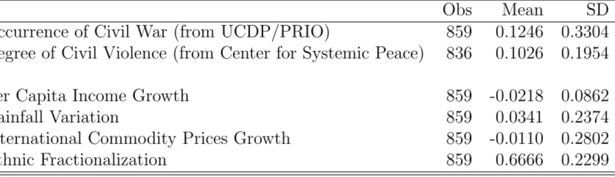
Table 1 presents descriptive statistics of Sub-Saharan Africa during 1981-2003. Along these 23 years, countries in this region have confronted 107 episodes of civil wars. On average, each country has an experience of civil war once in every ten years. This statistics is in line with the degree of civil violence from zero to one divided by one-tenth. The mean of the violence degree is around 0.1 and its range is around 0.2. Large range of deviation points out several degree of violence from the modest to the strongest ones. The correlation between the likelihood of civil wars and the degree of civil violence is at 72 percents indicating consistency between datasets from two sources.
Average income growth of the region is close to zero at -2.2 percentages annually. Its standard deviation has wide range at 8.6 percents or around 4 times of its mean, indicating the various characteristics of countries in Sub-Saharan Africa. This high range of income growth particularly comes from the high range of its determinants; commodity prices growth and rainfall variation. The average value of commodity prices growth is -1.1 percentages, while its standard deviation is around 25 times to its mean. Likewise, average value of rainfall variation is 3.4 percentages, while its standard deviation is almost 7 times. Henceforth, wide ranges of these determinants forward to high variability of income growth of the whole region.
However, wide range of Sub-Saharan African characteristics is not only based on income growth but also based on index of ethnic fractionalization. Mean of ethnic frac-tionalization index is reported at 0.667, while the minimum and maximum values are 0.036 and 0.925. This statistics indicates that the country composition of this region goes from almost unique-group country to almost scattered-group country.
4.2
First Stage Results
Table 2 shows the estimates of first-stage regression replicating several combinations of independent variables from the literature with the 1981-2003 dataset. Column (1) produces the link between rainfall variation at time t and t−1 replicating Miguel et al. (2004). The equation shows the positive statistical significance of contemporaneous and lagged rainfall variation. Ciccone and Br¨uckner (2010) adjusted Miguel et al. (2004)’s first stage equation by adding a variable commodity prices growth. They found as shown in column (2) that all three variables are statistically significant to instrument income growth. However, Br¨uckner and Ciccone (2011) revised their 2009 paper as shown in column (3) by eliminating rainfall variation to one variable commodity prices growth. The significance of this one instrumental variable case is still very strong.
Although these replicated first stage equations are statistically significance with in-dividual hypothetical testing for each independent variables, the overall testing of hy-pothesis needs to be evaluated. For the two stage least squared model with only one endogenous regressor, a rule of thumb criteria is a first-stage F statistics for weak instru-ments at least or around 10. The F-statistics and its p-value are reported at the bottom of each column in Table 2. Column (1) and (2) shows the replication of Miguel et al. (2004)’s and Ciccone and Br¨uckner (2010)’s first stage equations with 1981-2003 dataset. They report the value of F statistics 7.39 and 7.47, respectively, pointing out problem of weak instruments. The equation in column (3) replicating Br¨uckner and Ciccone (2011) by one instrumental variable commodity prices growth do not suffer by weak instrument problem, since its value of F statistics is 14.43 exceeding the criteria 10. So Br¨uckner and Ciccone (2011)’s first stage equation is one of baseline models in this paper.
According to column (1)-(3) replicated from the literature, the proper of first stage equation is based on statistical issue rather than economic issue. In Sub-Saharan Africa where is the world’s large agricultural exporter, the production of these countries pre-liminarily depends on rainfall variation. Then rainfalls is a reasonably significant deter-minant of income growth. This paper produces another combination of rainfall variation and commodity prices growth as shown in column (4). Both instrument variables are statistically significant and the overall equation does not have weak instrument problem with F statistics close to 10 which can be acceptable.
In sum, this paper uses two packages of instrument variables to estimate first stage equations passing through the second stage ones. The first package is taken from Br¨uckner and Ciccone (2011) with only one variable commodity prices growth, while the second one includes an additional variable rainfall variation.
Furthermore, the estimation including the interactions of income growth and ethnic fractionalization index needs another overall test of weak instruments problem. It is a case of more than one endogenous regressors. The criteria becomes Shea Partial R-squared. However, the formal critical value of Shea Partial R-squared has not yet academically concluded, most of the econometric papers accept this value at 0.05. These values are reported at the bottom of each column in Table 4.
4.3
Second Stage Results
Table 3 reports second stage results as baseline results. The relationship between the likelihood of civil wars and its determinants are reported in column (1)-(6), while the relationship between the degree of civil violence and its determinants are reported in column (7)-(12). The first three columns of each relationship are estimated by Br¨uckner and Ciccone (2011)’s first stage equation, and the last three columns are done by the first stage equation proposed by this paper. Moreover, each of the three columns of first stage equation are controlled by country fixed effects, specific time trends and common time dummies for unobservable factors, additionally.
Column (1)-(3) present OLS results linking the likelihood of civil wars with income growth. An increase of income growth is statistically significant to reduce the likelihood of civil wars around 30-35 percentage points. Br¨uckner and Ciccone (2011)’s first stage equations are employed for 2SLS estimates. The relationship of the likelihood of civil wars and income growth are still statistically significant but their values of coefficients are much higher, in absolute term, than the OLS estimation.
The estimates of this paper’s first stage equations linking the likelihood of civil wars and income growth are presented in column (4)-(6). The results are strongly significant as same as the Br¨uckner and Ciccone (2011)’s replication. These results are also tested against over-identification problem as reported at the bottom of each column indicating that they do not have this problem. In sum, income growth reduces the likelihood of civil wars as expected.
The OLS estimates of income growth on the degree of civil violence are presented in column (7)-(9). They show that an income growth decreases the degree of civil violence around 10 percentage points. After that, the 2SLS estimates based on Br¨uckner and Ciccone (2011)’s first stage equations show the opposite sign. They point out that an income growth increases the degree of civil violence, even if they are not statistically significant. Likewise, results based on this paper’s first stage equations confirm positive relationship of the degree of civil violence and income growth. They confirm the positive relationship as same as Br¨uckner and Ciccone (2011)’s equation without any statistical significance and overid problem. In short, after the correction of biasedness from two-way relationship, an income growth seems to increase rather than decrease the degree of civil violence.
4.4
Results on Heterogenous Growth Effects of Ethnic
Frac-tionalization
Table 4 reports results of heterogenous growth effects of ethnic fractionalization index on the likelihood of civil wars. The links of civil wars to income growth and its interaction with ethnic fractionalization index are reported in column (1)-(8), while the one of the
degree of civil violence and its determinants are reported in column (9)-(16). The first four columns of each relationship are estimated by Br¨uckner and Ciccone (2011)’s first stage equation, and the last four columns are by this paper’s first stage equation.
The 2SLS result of one regressor from income growth to the likelihood of civil wars by Br¨uckner and Ciccone (2011)’s first stage equation is shown in column (1). It indicates that an increase of income growth reduces the likelihood of civil wars . The heterogenous growth effects of ethnic fractionalization index on the likelihood of civil wars by Br¨uckner and Ciccone (2011)’s first stage equation are presented in column (2)-(4). They show the negative coefficients of stand-alone income growth and positive coefficients of its interaction with ethnic fractionalization index. It points out that income growth decreases the likelihood of civil wars by itself while the interactions indicates that there is a reverse effect in high ethnic fractionalized countries. These positive effects of the interactions are not statistically significant. However, the less values of interaction coefficients than the values of income growth coefficients indicate that income growth always reduce the likelihood of civil wars no matter what ethnic composition is.
Column (5) shows result from this paper’s first stage equation pointing out negative effects of income growth on the likelihood of civil wars . The interaction effects of income growth and ethnic fractionalization index on the likelihood of civil wars are reported in column (6)-(8). The results are almost in line with the ones with Br¨uckner and Ciccone (2011)’s first stage equation showing the negative coefficients of stand-alone income growth and positive coefficients of its interaction. However, these results show statistical significance of interaction variables confirming heterogenous growth effects of ethnic fractionalization index. As Br¨uckner and Ciccone (2011)’s first stage equation, the less values of interaction coefficients than the values of income growth coefficients indicating that income growth always reduce the likelihood of civil wars . The over-identification tests at the end of each column show no problem.
The link of the degree of civil violence to income growth without an interaction is reported in column (9). It shows that an income growth increases the degree of civil violence with no statistical significance. After adding the interaction with ethnic
tionalization index in column (10)-(12), the coefficients of income growth are positive and the coefficients of interactions are negative. An income growth increases the degree of civil violence by itself, while the effect of ethnic fractionalization decreases it. Due to less value of stand alone coefficients than their interactions, an increase of income growth reduces the degree of civil violence in the low ethnic fractionalized countries while it increases in the high ethnic fractionalized countries.
Column (13) shows the relationship between the degree of civil violence and income growth by this paper’s first stage equation. The result points out positively statistical insignificance. After adding interactions, the results turn to be statistical significance and are in line with the case of Br¨uckner and Ciccone (2011)’s first stage equation showing the coefficients of income growth are positive and the coefficients of interactions are negative. It indicates that an increase of income growth reduces the degree of civil violence in the low ethnic fractionalized countries while it increases in the high ethnic fractionalized countries. There is no over-identification problem.
The interpretation of these results can be probably based on market competition model. The market with few large producers may be more competitive than many small producers to be market leader. As in the political market, when economy grows, few large ethnic groups probably are more powerful and higher potential to compete for occupying government power than many small ethnic groups. Many small groups own too less resources and difficult to cooperate to clash with their big government. This is partly because the inefficient income distribution mechanisms in this region because excess benefit can be taken by the one who controls government power.
5
Concluding Remarks
The intuition of this paper is based on the question whether an increase of income growth affects the likelihood of civil wars different in ethnic fractionalization. This paper defines two dimensions of civil wars; its number and violent degree. The method of es-timation is instrument-variable two-stage-least-squared technique to overcome causality
problem. The commodity prices growth and rainfall variation are employed as instru-ments in the first stage with strongly statistical significance. Also the statistics reports that they have no over-identification problem.
Results coincide with literature that income growth always reduces the likelihood of civil wars. However, countries with few large ethnic groups get more reduction than countries with many small groups when income grows. This result is partly opposite to the result of the degree of civil violence. An income growth increases the degree of civil violence in the few large ethnic groups countries, while it decreases the degree in the many small ethnic groups ones.
In general, an increase of income growth reduces both the likelihood of civil wars and the degree of civil violence in the many small ethnic groups countries. So income growth is good in reduction of civil wars in both dimensions. In few large ethnic groups countries, an increase of income growth reduces the likelihood of civil wars and but increases the degree of civil violence. It is therefore like a trade-off between number and violent level of civil wars in these countries.
The policy implication from this paper points out that growth promotion may not always be beneficial to every country with civil wars. If the occurrence of civil wars is counted in number, income growth advancement seems to be advantageous. But in the few large ethnic groups countries, income growth creates more incentive to the other ethnic groups out of government power to grasp this power which they are high potential to defeat. The degree of violence would be higher, then countries would be more suffered from higher degree of violence even less amount of wars. Hence, effective policy to promote income growth for reducing civil wars needs to concern ethnic fractionalization.
References
Acemoglu, D. (2005). Evaluation of World Bank Research. in A. Deaton, K. Rogoff, A. Banerjee, N. Lustig, eds. Evaluation of World Bank Research Over the Last Decade.
Br¨uckner, M. and A. Ciccone (2010) ”International Commodity Prices, Growth and Civil Wars in Sub-Saharan Africa” The Economic Journal 120 (544): 519-534.
Ciccone, A. and Br¨uckner, M. (2011) ”Rain and the Democratic Window of Opportunity” Econometrica 79 (3): 923-947.
Collier, P. and A. Hoeffler (1998). On Economic Causes of Civil War. Oxford Economic Papers 50 (3): 563-573.
Collier, P. and A. Hoeffler (2004). Greed and Grievance in Civil War. Oxford Economic Papers 56 (4): 563-596.
Easterly, W. and R. Levine (1997) Africas Growth Tragedy: Policies and Ethnic Divisions Quarterly Journal of Economics 112 (4): 12031250.
Fearon, J. and D. Laitin (2003). Ethnicity, Insurgency and Civil War. American Political Science Review 97 (1): 75-90.
Hegre, H. and N. Sambanis (2006). Sensitivity Analysis of the Empirical Results on Civil War Onset. Journal of Conflict Resolution 50 (4): 508-535.
McGowan, P. and T.H. Johnson (1994) ”African Military Coup d’etat and Underdevel-opment: A Quantitative Historical Analysis” Journal of Modern African Studies, 22 (4): 633-66.
Miguel, E., S. Satyanath, and E. Sergenti (2004). Economic Shocks and Civil Conflict: An Instrumental Variables Approach. Journal of Political Economy 112 (41): 725-753. Sambanis, N. (2002). A Review of Recent Advances and Future Directions in the Quan-titative Literature on Civil War. Defence and Peace Economics 13 (3): 215-243.
United Nations Conference on Trade and Development (2009). Commodity Price Series. Online Database.
World Bank (2003). Breaking the Conflict Trap: Civil War and Development Policy. Oxford University Press.
Table 1: Descriptive Statistics
Obs Mean SD
Occurrence of Civil War (from UCDP/PRIO) 859 0.1246 0.3304 Degree of Civil Violence (from Center for Systemic Peace) 836 0.1026 0.1954
Per Capita Income Growth 859 -0.0218 0.0862
Rainfall Variation 859 0.0341 0.2374
International Commodity Prices Growth 859 -0.0110 0.2802
Ethnic Fractionalization 859 0.6666 0.2299
T able 2: First Stage Equations Income Gro wth Miguel et al. (2004) Ciccone and Br ¨uc kner (2010) Br ¨uc kner and Ciccone (2011) New Com bination (1) (2) (3) (4) Rainfall V ariation 0.053*** 0.049** * 0.036** (0.015) (0.016) (0.014) Lagged Rainfall V ariation 0.038 *** 0.035* * (0.013) (0.015) Commo dit y Prices G ro wth 0.039*** 0.038*** 0.039*** (0.01) (0.01) (0.01) F-statistics (Instrumen t = 0) 7.39 7.47 14.43 9.88 p-v alu e (0.00 19) (0.0005) (0.0005) (0.0004) R-squared 0.0807 0.1321 0.1199 0.1272 Cross Coun try Fixed Effects Y Y Y Y Sp ecific Time T rends Y Y Y Y Common Time D ummies N Y Y Y Note: The metho d of estimation of the first stage equations is least squares. Hub er robust standard errors (in paren theses) are clustered at the coun try lev el. The mo de ls w ere replicated from the literature of instrumen tal v ariable approac h from income gro wth to the lik eli h o o d of civil w ars in Sub-Saharan Africa; Miguel et al. (2004), Ciccone and Br ¨uc kner (2010) and Br ¨uc kner and Ciccone (2011), resp ectiv ely from column (1)-(3), with the dataset 1981-2003. Also thi s pap er pro vides new com bination of indep enden t v ariables from the literature in column (4). Commo dit y Prices Gro wth is the commo dit y price gro wth rate b et w een t and t-3, using in ternationa l commo dit y price data from IMF. F statistics and its p v alue are rep orted to test against all instrumen ts are con trolled. Cross coun try fixed effe cts, sp ecific time trends and common time dummies are con trolled as indicated at the b ottom of e a ch colum n . *Significan tly differen t from zero at the 90 p ercen t confidence lev el, ** 95 p ercen t confidence lev el, *** 99 p ercen t confidence lev el.
T able 3: Baseline Equations Occurrence of Civil W ars Degree of Civil Violence Br ¨uc kner and Ciccone (2009)’s IV New Com bination’s IV Br ¨uc kner and Ciccon e (2009)’s IV New Com bination’s IV (1) (2) (3) (4) (5) (6) (7) (8) (9) (10) (11) (12) OLS Estimates Income Gro wth -0.349*** -0.3 34*** -0.306*** -0.349*** -0.334*** -0.306*** -0.119** -0.103* -0.090* -0.119** -0.103* -0.090 * (0.105) (0.102) (0.096) (0.105) (0.102) (0.096) (0.058) (0 .057) (0.051) (0.058) (0.057) (0.051) R-squared 0.3777 0.4485 0.4799 0.3777 0.4485 0.4799 0.5305 0.6137 0.619 0.5305 0.6137 0.619 Reduced F orm Estimates Commo dit y Prices Gro wth -0.096*** -0.103*** -0.092** -0.096** * -0.103*** -0.091** 0.018 0.016 0.019 0.019 0.016 0.01 9 (0.035) (0.036) (0.036) (0.035) (0.036) (0.036) (0.021) (0 .022) (0.026) (0.021) (0.022) (0.026) Rainfall V ariation -0.035* -0.024 0.017 -0.009 -0.001 0.007 (0.019) (0.019) (0.018) (0 .013) (0.0 14) (0.01 5) R-squared 0.3764 0.4487 0.4782 0.377 0.449 0.4783 0.5 286 0.61 23 0.6181 0.5287 0.6123 0.6182 2SLS Estimates Income Gro wth -2.3 08** -2.441** -2.368** -1.706*** -1.687*** -1.200** 0.454 0.386 0.508 0.171 0.2 12 0.377 (0.950) (0.978) (1.056) (0.619) (0.639) (0.607) (0.482) (0 .495) (0.657) (0.323) (0.332) (0.424) Ov erid 1 .2905 2.19828 3.4288 1.12534 0.52361 0.142054 p-v alu e (0.256) (0.138) (0.064) (0.289) (0.469) (0.706) First Stage Estimates Income Gro wth Commo dit y Prices Gro wth 0.0 41*** 0.042*** 0.038* ** 0.041*** 0.042*** 0.039*** 0.041*** 0.042*** 0.039*** 0.041*** 0.042 *** 0.038*** (0.009) (0.009) (0.010) (0.009) 0.010 0.010 (0.009) (0.010) (0.010) (0.009) 0.010 (0.010) Rainfall V ariation .041*** 0.041*** 0.036** 0.042*** 0.042*** 0.036*** (0.013) 0.014 (0.014) (0.013) (0.014) (0.014) First Stage F-statistics 27.97 17467.08 67.46 1 9.49 9 8.12 106.81 13 .1 17434 .45 252.36 9.17 96.59 103.3 F-statistics (Instrumen t = 0) 18.5076 17.7785 14.4318 11.3583 10.4865 9.88 17.8702 10.2654 13.5246 11.0997 10.2654 9.446 Coun try Fixed Effects Y Y Y Y Y Y Y Y Y Y Y Y Sp ecific Time T rends N Y Y N Y Y N Y Y N Y Y Common Time Dummies N N Y N N Y N N Y N N Y Note: The metho d of estimation of the first stage equations is least squares. Hub er robust standard errors (in paren th e ses) are clustered at the coun try lev el. The mo dels w ere replicated from the literature of instrumen tal v ariable appro ac h of Br ¨uc kner and Ciccone (2011) in column (1)-(3) and (7)-(9), w ith the dataset 1981-2003. Also this pap er pro vides new com bination of instrumen t v ariables from the literature in column (4)-(6) and (10)-(12). Commo dit y Prices Gro wth is the comm o dit y price gro wth rate b et w een t and t-3, using in ternational commo di ty price data fro m IMF. F statistics and its p v alue are rep orted to test against all instrumen ts ar e con trolled. Cro ss coun try fixed e ffects, sp ecific time tr e nd s and common time dummies are con trolled as indicated at the b ottom of eac h column. * Si g nific a n tly differen t from zero at the 90 p ercen t confidence lev el, ** 95 p ercen t confidence lev el, *** 99 p ercen t confidence lev e l. 17
T able 4: Equations with the Heterogeneous Gro wth Effect Num b er of Civil W ars Degree of Civil Violence Br ¨uc kner and Ciccone (2009)’s IV New Com bination’s IV Br ¨uc kner and Ciccone (2009)’s IV New Com bination’s IV (1) (2) (3) (4) (5) (6) (7) (8) (9 ) (10) (11) (12) (13) (14) (15) (16) 2SLS Estimates Income Gro wth -2.368** -3.928* -4.021* -3.942* -1.200** -3.827*** -3.953*** -3.105** 0.508 2.749*** 2.782*** 2.913*** 0.377 1.898** 1.882** 1.984** (1.056) (2.258) (2.277) (2.151) (0.607) (1.524) (1.500) (1.274) (0.657) (0.978) 0.990 (1.073) (0.424) (0.908) (0.921) (0.899) Income Gro wth x Indicator for: 2.628 2.552 2 .440 3.33 6* 3.579** 3.084* -3.749*** -3.895*** -3.743*** -2.540** -2.430** -2.334** Ethnic F ractionali zation (3.174) (3.155) (2.875) (2.008) (1.950) (1.890) (1.338) (1.353) (1.238) (1.213) (1.226) (1.132) Ov erid 1.08224 2.16947 4.099 69 3.63732 4.49568 4.17308 p-v alu e (0.582) (0.338) (0.129) (0.162) (0.106) (0.124) First Stage Estimates Income Gro wth Commo dit y Prices Gro wth 0.038*** 0.050*** 0.049*** 0.0 47*** 0.039*** 0.051*** 0.049*** 0.048*** 0.038** * 0.051*** 0.049*** 0.047** 0.038*** 0 .051*** 0.049*** 0.047*** -(0.010) (0.016) (0.016) (0.018) (0.010) (0.016) (0.016) (0.017) (0.103) (0.016) (0.016 ) (0.018) (0.424) (0.016) (0.016) (0.018) Commo dit y Prices Gro wth x -0.014 -0.010 -0.014 -0.015 -0.0 10 -0.01 4 -0.014 -0.010 0.026 -0.015 -0.010 -0.014 Indicator (0.024) (0.025) (0.026) (0.024) (0.024) (0.025) (0.024) (0. 025) (0.024) (0.025) (0.026) Rainfall V ariation 0.036** 0.019 0.018 0.022 0.036** 0.018 0.017 0.02 (0.014) (0.043) (0.044) (0.044) (0.014) (0.043) (0.044) (0.045) Rainfall V ariation x 0.033 0.035 0.021 0.037 0.039 0.025 Indicator (0.068) (0.071) (0.071) (0.069) (0.071) (0.072) First Stage F-statistics 67. 46 19.23 11768.22 104.66 106.81 12.3 342566.92 623.06 90.49 27.6 11749.99 280.7 103 .3 6.32 342785.27 392.29 Shea P artial R-squared 0.037 0.0364 0.0322 0.0445 0.0438 0.0421 0. 0371 0.0365 0.0322 0.044 7 0.044 0.0424 Income Gro wth x Indicator Commo dit y Prices Gro wth -0.001 -0.002 -0.002 -0.001 -0.002 -0.002 -0.001 -0.002 -0.002 -0.001 -0.002 -0.002 (0.007) (0.007) (0.009) (0.006) (0.007) (0.009) (0.007) (0.007) (0.009) (0.006) (0.007) (0.009) Commo dit y Prices Gro wth x 0.042*** 0.045*** 0.043*** 0.042*** 0.045*** 0.043*** 0.042*** 0.045*** 0.044*** 0.042*** 0. 045*** 0.044*** Indicator (0.014) (0.015) (0.014) (0.014) (0.014) (0.014) (0.015) (0. 015) (0.015) (0.014) (0.015) (0.015) Rainfall V ariation -0.010 -0.011 -0.010 -0.012 -0.013 -0.012 (0.018) (0.019) (0.022) (0.018) (0.019) (0.022) Rainfall V ariation x 0.06 0.062 0.052 0.063 0.065 0.055 Indicator (0.039) (0.042) (0.043) (0.040) (0.042) (0.045) First Stage F-statistics 67. 46 17.48 14686.68 323.4 5.46 7 17596.02 1247.17 26.68 5502.79 433.8 5.23 718815.55 1183.55 Shea P artial R-squared 0.033 9 0.0344 0.0359 0.0443 0.0446 0.0443 0.0339 0.0345 0.0359 0.0449 0.0453 0.0456 Coun try Fixed Effects Y Y Y Y Y Y Y Y Y Y Y Y Y Y Y Y Sp ecific Time T rends Y N Y Y Y N Y Y Y N Y Y Y N Y Y Common Time Dummies Y N N Y Y N N Y Y N N Y Y N N Y Note: The metho d of estimation of the first stage equations is least squares. Hub er robust standard errors (in paren th e ses) are clustered at the coun try lev el. The mo dels w ere replicated from the literature of instrumen tal v ariable approac h of Br ¨uc kner a nd C iccone (201 1) in column (1)-(4) and (9)-(12), with the dataset 1981-2003. Also this pap er pro vides new com bination of instrumen t v ariables from the literature in column (5)-(8) and (13)-(16). Commo dit y Prices Gro wth is the comm o dit y price gro wth rate b et w een t and t-3, using in ternational commo di ty price data fro m IMF. F statistics and its p v alue are rep orted to test against all instrumen ts ar e con trolled. Cro ss coun try fixed e ffects, sp ecific time tr e nd s and common time dummies are con trolled as indicated at the b ottom of eac h column. * Si g nific a n tly differen t from zero at the 90 p ercen t confidence lev el, ** 95 p ercen t confidence lev el, *** 99 p ercen t confidence lev e l.
Second Paper
The Diffusion of Civil War and Peace
in Sub-Saharan Africa
Thanee Chaiwat
∗June 7, 2013
Abstract
This paper investigates the clustering and contagion of civil conflicts in Sub-saharan Africa using spatial panel data models. The results document that onset, incidence and end of civil conflicts spread across the network of neighboring countries while peace, the end of conflicts, diffuse only with the nearest neighbor. In term of space, these results also confirm the clustering of civil war incidence. Finally, there is an evidence of indirect links from regional income growth, without too much inequality, of neighbor countries to reduce the likelihood of civil wars.
JEL-classification: C23, D74, R12
Keywords: Civil War; Africa; Geography; Cluster; Diffusion; Spatial Analysis; Contagion Process
∗PhD student at University of Bologna. [email: thanee.chaiwat2@unibo.it] I am grateful to my
su-pervisor Matteo Cervellati, to Roberto Patuelli, Simona Valmori, Francesco Manaresi and Maria Giulia Silvagni for useful suggestions and to Carlo Gaeton for helps with the statistics packages for spatial econometrics. All errors are mine.
1
Introduction
Civil wars are the most common type of armed conflicts in the last half-century accounting for large human and economic disruption. Since 1960s about twenty percents of countries have experienced at least ten years of civil wars. The plague of violent civil strives is particularly cumbersome for Sub-Saharan Africa where more than one third of the countries experienced at least a civil war during even the past twenty years.
A large body of empirical literature, discussed in more detail in Section 2, investigates the determinants of civil wars. Most of the available investigations have concentrated their attention to the study of country specific characteristics that and/or the role of short term climatological and economics shocks increase the likelihood of conflicts and more recently some studies has turned to the investigation of the ”non domestic” determinants of civil conflicts with a special attention to the role of clustering and diffusion among neighboring countries. The results of these investigations deliver mixed findings. The available investigations mostly favor territorial neighboring concept, focusing on war onset as a dependent variable.1
This paper investigates the clustering and contagion of civil conflicts in both space and time using recently developed spatial panel data techniques. The results complement the existing literature in four main dimensions. First, the role of spatial connections be-tween countries is accounted for by using several methods to define the relevant neighbor network.2 The consideration of different possible network structures allows to investigate different possible patterns of clustering and contagion. By employing these several con-cepts with the same model specification, the paper provides systematic and comparable estimates. The results suggest that the definition of the relevant network may play a key role with respect to the pattern styles of diffusion process.
1The results in the literature, reviewed in more details below, use different data, alternative definitions
of conflict and explanatory variables, different spatial weighting schemes and time periods such as post WWII or post Cold War.
2As discussed in detail in Section 4.2, the first neighboring method is traditional definition accounting
for countries who share common borders. The second method, called distance-based, is based on distant area. Countries within circular area from the centroid of each country are included as neighbors. The last method, called one-nearest, takes into account for one country which locates the nearest, in term of distance among centroids, to each other.
Second, the paper investigates different dimensions of conflicts including their onset, incidence and end. This allows for a first test of the different pattern of clustering and contagion of the different phases of conflicts which, to our knowledge, was not investigated in the literature. The findings provide evidence of asymmetric diffusion patterns. While the start, and incidence of civil wars tend to diffuse in circular directions, the end of conflicts, or alternatively if we want the start of peace, tends to diffuse only to the nearest neighbor. This paper suggests that war diffuse more widely than peace does.
Third, the analysis explicitly studies role of time by including the different lagged spatial variables in the panel data estimation. A variety of specifications is considered to investigate the time it takes to diffuse and the duration of the effects. The asymmetry between start (or incidence) and end of conflicts emerges not only in terms of space but also in terms of time. The civil wars need only one year to diffuse and they significantly spread for about two years. In contrast, peace need two years to diffuse and the effect last less (only one year).
Finally, this paper also studies the possibility of indirect diffusion channel across coun-tries. In particular, the analysis allows for the possibility that better economic conditions in neighboring countries may indirectly help limiting conflicts. The findings document that while income growth in a country has negative correlation with the likelihood of civil war, there is an evidence that effects of economic well-being on conflicts diffuse to other countries as well. The models show significant links from neighbors’ income growth both onset and end phases of civil wars. This results provide a set of novel insights and may have relevant policy implications.
2
Related Literature
Most of the studies of civil war investigates domestic socio-economic conditions as its de-terminants, for example, per capita income growth, quality of political institutions, acces-sibility of natural resources, ethnic fractionalization and climatological shocks. Probably, the most acceptable key factor reducing civil wars is income growth [Collier and H¨oeffler (1998); Collier and H¨oeffler (2002); Miguel, Satyanath and Sergenti (2004) and Br¨ukner and Ciccone (2010)]. According to Blattman and Miguel (2010), “the correlation between
low per capita incomes and higher propensities for war is one of the most robust empir-ical relationships in the literature”. Other factors beyond socio-economic condition were also related to domestic concept such as political regime type, governmental instability and population density [Benson and Kugler (1998); Collier and H¨oeffler (2004); Sambanis (2004); Gleditsch (2007)]. These aspects are not very different in the case of civil war onset, incidence, and termination.
Early works in the spatial analysis of civil war focus how neighboring states influence the propensity to the spread of international wars. This analysis is the consequence of merger of international relations theory and spatial analysis which rediscovered the importance of contiguous effects in the diffusion of conflict, as elaborated in Most and Starr (1980). In their formulation, country’s borders offer opportunities for conflict (more borders, more conflict possibilities); the sense of vulnerability from multiple borders can lead to military preparations and a willingness to fight. Most and Starr’s diffusion analyses relied on simplified contiguity scores for states (the so-called checkerboard measure in spatial autocorrelation analysis). Their analyses of global and African wars [Starr and Most (1983)] found high correlation between international wars among border sharing countries. Kirby and Ward (1987) also confirms that in Africa neighboring influence is stronger than the effect of domestic characteristics in determining war risk.
Later, the studies extended their analysis to the impact of neighbors on the likelihood of civil wars by neighboring state factors. The results, to date, have been inconclusive partly due to different empirical specifications including different data sets, with differ-ent definitions of conflict and explanatory variables, use of differdiffer-ent spatial weighting schemes and time periods. While a number of researchers dismiss the effect of neighbors in increasing or decreasing civil war risk [Fearon and Laitin (2003)], others find strong support for neighboring effects on civil war risk when controlling for the usual explanatory variables including GDP, political regime type, governmental instability and population density [Benson and Kugler (1998); Collier and H¨oeffler (2004); Sambanis (2004); Gled-itsch (2007)].
Gleditsch (2002) found that neighboring and regional relationships set the trajectory (peaceful or conflictional) for individual states. States in high-risk regions experience “double jeopardy”, as their unstable domestic politics result in high civil war risk that
neighbors with high domestic risk compound. Hence, within developing countries, do-mestic politics are as much influenced by external relationships as by internal political, economic and social dynamics. Gleditsch (2007) extended his work that transnational linkages between states and regional factors strongly influence the risk of civil conflict such as trans-border groups, regional trade and regional democracy.
Buhaug and Gleditsch (2008) also tested whether conflicts are clustered by themselves or due to the agglomeration of poverty in some regions. data on civil conflicts at the country level around the world and found that conflicts are still clustered by themselves even if the poverty was controlled for. Similarly, the study of disaggregate level by Buhaug and Rød (2006) detected spatial conflict clusters in the disaggregate level using data on civil conflicts for Africa using 100x100 km grid cells and regional conflicts’ location during 1970-2001. Therefore these studies make conclusion about the existence of cluster, but they don’t clarify its contagion process. The occurrence of cluster may not be necessary to point out the phenomenon of diffusion. The existence of diffusion need to be supported by contagion process in which the role of time must be involved, nevertheless the cluster may exist by the cluster of exogenous factors.
Scutte and Weidmann (2011) theoretically points out two types of diffusion pattern. How civil wars diffuse can be either moving or expanding themselves. They interpret contemporaneous spatial variables together with the lagged ones to identify each type of diffusion pattern. If wars are contagious among neighbors, either the existence of cluster can identify the escalation diffusion or the existence of checkerboard can identify the relocation diffusion. This study finds some cases proven by this theoretical point of view and will discuss later in section 4.1.
Section 2 and 3 provide a detail of spatial econometric methodology; data measure-ment and empirical strategy. The fifth section is empirical results and the last section is concluding remarks.
3
Data and Measurement
The period of analysis ranges from 1981 to 2003. Most of Sub-saharan African countries were independent and majority ruled before 1980 [McGowan (2003)], then year 1981
kicked off the second democratization wave in Africa. This paper covers a sample of 37 countries in Sub-saharan Africa.3
Civil Wars: Data on civil wars is extracted from the UCDP/PRIO Armed Conflicts Dataset of the International Peace Research Institute’s (PRIO) Centre for the Study of Civil War and the Uppsala Conflict Data Program (UCDP).4 The UCDP/PRIO Armed
Conflict Database defines civil war as a “contested incompatibility which concerns gov-ernment and/or territory where the use of armed force between two parties, of which at least one is the government of a state, results in at least 1000 battle deaths per year”.5
This paper studies the occurrence of civil wars based on PRIO’s definition and catego-rized into three variables. The first variable iscivil war incidence, denoted byincidence
as defined in PRIO. It takes value one in year of civil wars occurred, otherwise it is coded zero. Hence the variable civil war incidence represents the whole period of war events.
The second variable is civil war onset, denoted by onset. The definition of this variable indicates the year wars start, so it is coded by the year changing values of the variable war incidence from zero to one, otherwise it is coded zero. It registers a shift from no war to war events at the first year. The definition of variable war start is different from the definition of war onset used in many papers. The variable war onset equals to one at the first year wars start, missing values at the year of war ongoing and zero at the year without war. But the spatial panel data analysis does not allow for missing values due to float of diffusion effects, the variable war start must not have any missing values. Hence the difference between variable war onset and variable war start is how to code at the years war ongoing with missing values and zero values respectively. However, the alternative way is to code 0 for all country-years with no war, 1 for the year that a war started, and missing for periods of ongoing war, but countries with ongoing wars will lose a lot of observations and this coding is not allowed in spatial panel data analysis.
3Only four countries of Sub-saharan Africa which are Zimbabwe, Namibia, Eritrea and South Africa
were independent after 1980 at different years, hence most of the studies started their analysis at 1981. There are 43 data-available countries in Sub-saharan Africa. Six omitted countries from this paper are Djibouti, Eritrea, Equatorial Guinea, Lesotho (due to incomplete data), Somalia (due to unavailable information) and Madagascar (due to island-being isolation).
4The dataset is available at http://new.prio.no/CSCW-Datasets/Data-on-Armed-Conflict.
5The definition of civil wars is exactly the same as civil conflicts. Civil conflicts count 25 to 999
battle-related deaths per year, while civil wars count more than 1,000 deaths.
The variable civil war end, denoted by end, is the third dependent variable in this paper. This variable is the opposite of the variable war onset. It takes value one in years of incidence shifting form one to zero, otherwise it is coded zero. It means the situation shifting from war events to no war at the first year. In this paper, peace is defined as the absence of wars, so the variable peace start is identified by the first year after war has stopped.
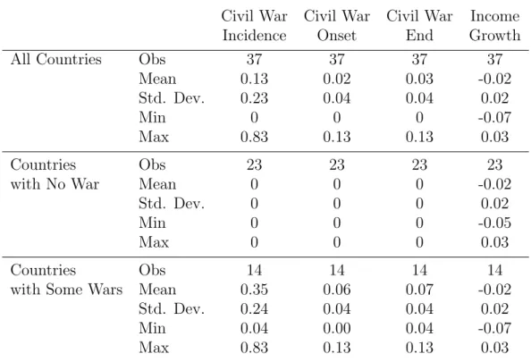
Descriptive statistics of the variable civil wars are reported in Table 1. They are for the whole region and for the classification by the occurrence of wars. It categorized into two groups; countries with no war and countries with some wars. On average for the whole region, the incidence of civil wars in Sub-saharan Africa was about 0.13 over the period 1981-2003. The mean values of variable war onset and war end are around 0.02 and 0.03 respectively.
Partitioning countries with and without civil wars, 23 out of 37 countries had not experience any war while 14 countries have at least one such war. The mean value of variable war incidence only the case of war countries appears much higher being at 0.35. It means that the probability of wars exists for each of such 14 countries at 35 percents per year. In the meantime, the mean probability of war start and war end increase at 0.06 and 0.07 respectively. For instance, the country Sudan, which has the maximum value of variable civil war incidence (0.83), had experienced civil wars almost the whole length of the study.
Income Growth: Data for annual real GDP per capita growth is taken from the World Development Indicators (2010).6 Table 1 provides some descriptive statistics of per capita income growth. The average income growth for the whole region was around -2 percents and ranged between -7 to 3 percents. When statistics are disaggregated between countries with no war and countries with some wars, the average values of growth are significantly different. Countries with no war grew at 2 percents on average per year, in contrast countries with some wars grew of (-2) percents per year.
4
Empirical Strategy
4.1
Estimation Framework
The benchmark equation links the likelihood of civil wars to per capita income growth, country characteristics, country specific time trends and common time dummies;
wari,t =βi,tgrowthi,t +µi+γit+δt+ui,t, (1)
where i indicates country of interest and t indicates year. The variable civil war, stated
war from now on, can be replaced by the variable war incidence, war start or war end in each of specific models. The variable growth is per capita income growth rate, µi is
time-invariant dummies, γit is a specific time trend, δt is common shock for each specific
year, and ui,t is an error term.
This estimation technique aims to overcome one of the traditional assumptions of ordinary least squares which presumes no correlation between error terms (corr(εi, εj)6=
0), particularly, among locations. In accordance with the literature, a civil war event is one case which violates this assumption. War in a specific location can affect and be affected by surrounding wars. However the effect among these locational spreads may take time, and the diffusion may not be observed at the static analysis. Inclusion of time will illustrate the escalation or movement of civil wars among spaces, then the main advantage of spatial panel data model is a capability to estimate the effects of space and time dimensions at the same time.
Therefore, the benchmark model is extended to Durbin spatial panel data model to propose space-time filter and allows for the spatial error correlation;
wari,t =ψ0Wij.warj,t+ψsWij.warj,t−s+βt−1growthi,t−1+θsWij.growthj,s+µi+γit+δt+it,
(2) wheret=νi,t+λWij0 .j,t andνt=ρνt−1+et. The spatial weight matrix, denoted by Wij,
is to identify neighbors and their weights inside. The spatial weight matrix for error term is denoted byWij0 , and the lagged year is indicated by s ranging from one to three.
In equation (2), the variable domestic income growth at time t −1 is linked to the likelihood of civil wars at timet. This is to limit causality problem of two-way relationship between contemporaneous income growth and the occurrence of civil wars. Additionally,
if the spatial weight matrix is equal to the spatial weight matrix for error term, that is
Wij = Wij0, there might be an identification problem. The values of interaction between
Wij0 and the disturbances may correlate with the values of interaction between Wij and
other independent variables. The estimation will be under the correlation between some regressors and error term, therefore the identification problem emerges. This paper con-trives the spatial weight matrix for error term different from the spatial weight matrix for other regressors, indeed Wij0 6=Wij. The concept of spatial weight matrices in the model
will be discussed in the next chapter.
Moreover, the presence of the variable war on both the left and right sides complies that least-squared estimates will be biased and inconsistent. The maximum likelihood estimation method used in this paper for evaluating the diffusion effects is therefore more suitable than the ordinary least square (LeSage (1998) and Bivand (2008)). According to LeSage and Pace (2009) and Elhorst (2010), the coefficient ψ is interpreted as “direct diffusion effect” linking neighbors’ war to our war in this case. The impact of domestic growth on the likelihood of civil wars is estimated by the coefficient β. The coefficient θ
is defined as “indirect diffusion effect” linking neighbors’ income growth to our war. The coefficient ψ0 indicates the probability of the existence of wars both in countries
and neighbors in the same year. This coefficient is interpreted as the likelihood of the cluster of civil wars. The concept of cluster is the agglomeration of similar events in space. A positive value of the coefficient ψ0 means high or low values of the variable
civil war events tend to cluster in space. That is countries either with or without civil wars are likely surrounded by similar neighbors. Yet a negative value of the coefficientψ0
means that our location tends to be surrounded by neighbors with dissimilar values, like a checkerboard. In other word, countries with civil wars are likely to be surrounded by neighbors without civil wars, or vice versa.
Since the diffusion process needs time to be contagious, the cluster coefficientψ0 which
is based on static period does not necessary allow to draw conclusion about the existence of the diffusion effect. The coefficientψs measures the relationship between the likelihood
of civil wars between countries and neighbors over time. For example, in the case of s
equals to one, the contagion coefficient ψ1 can be interpreted as the probability of our
be infected wars of our country this year from surrounding wars last year. The statistical significance of this coefficient in each period indicates how long the likelihood of civil wars spreads among neighbors.
The contagion coefficient variable is very important to confirm the presence of diffusion effects. The statistical significance of the cluster coefficient alone does not always point out the diffusion effect, because other independent variables may lead to the clustering of civil conflicts. For example, the cluster of war may exist due to the cluster of low income countries, not by war itself. In contrast, if the contagion coefficient is statistically significant and the cluster coefficient is not, diffusion can still be explained.
As in Schutte and Weidmann (2011), diffusion processes refer to dynamic changes both spatially and temporally, since the process of infection typically takes time. The spatial diffusion by this concept somehow is divided into two patterns. Firstly, the escalation diffusion pattern implies the expansion of the geographic scope from one location to a new location expanding from previous locations. This pattern emerges if the existence of the cluster of wars together with the positive contagion process. In equation (2), the statistical significance should appear on both a positive value of cluster coefficientψ0 and
a positive value of contagion coefficient ψs. Secondly, the relocation diffusion pattern
is generated by the movement of wars beyond the original location with later ending of wars at the previous locations. This pattern is observed if the existence of the contagion process at the same time with the checkerboard of wars because the previous wars had to stop later. To detect such a pattern, a positive value of contagion coefficient ψs and a
negative value of cluster coefficient ψ0 need to be statistically significant in the equation
(2).
4.2
Spatial Weight Matrix
To define neighboring countries, this paper uses three methods.
The first one is the Contiguity Queen Neighboring Method.7 Countries sharing
common borders are defined neighbors. The particular definition of border applies to country not only connected by land, but also to country divided by river, lake, mountain
7This method is called Queen because it is referred to the queen in chess playing which can move in
every direction. There are also Rook and King concepts to differentiate direction of movement.
or any other partitions. This concept focuses on the territorial line of each observation, but varies in the number of links and distance.
Second, the Distance-based Neighboring Method counts countries as neighbors if their centroid points are within distant band. To avoid that some countries have no neighbor, this paper specifies the maximum distance between the centroid of two border-sharing countries as the distant band. Distance-based neighbors implies the constantly distant radius from specific location, but varies in the number of links without concerning any contiguity.
The third method is the Nearest Neighboring Method. This method counts as neighbor only the nearest country measuring the distance between two centroids. Hence it specifies the exact amount of links which is one in this paper, but varies in distance without concerning contiguity. Besides this method can specifies any numbers of nearest neighbors and this paper specifies only one, so from now on it is called one-nearest neighbor.
This paper applies all three methods to create spatial weight matrix in each specific equation. However the models also need another spatial weight matrix to allow for spatial diffusion of error term. At the same time, the estimation has to be aware of a potential identification problem which is the correlation between spatial error term and other re-gressors. This paper employs second-degree contiguity queen neighbors, two layers of border sharing countries for the spatial weight matrix of error term.
Figure 1 shows the links resulting for each type of neighbor matrix. Each of the nodes represents the centroid of each country, so one country has only one node. Each line shows the links among neighboring countries. Within distant band, smaller countries tend to be clustered more than bigger ones. There are more numbers of neighbors for smaller countries in the distance-based neighboring method, while size of the countries does not affect the number of links in other neighboring methods.
The summary statistics of the number of links is presented in Table 2. There are 37 countries in each neighboring matrix. The average number of border sharing neighbors for one country is 4.3, while the average for distance-based method is 5.9 neighbors. Since the distance-based neighboring method covers larger area than the other methods, it includes as much as 220 neighbor links. Contiguity queen and one-nearest neighboring methods result in 160 and 37 links, respectively.
To specify spatial weights to neighbor relationship, this paper uses row standardized method. This method identifies each weight by the average value across the total amount of neighbors of each country. For example, countries with four neighbors will have the value one-forth for each weight. The concept behind this weighting method is the lower is the number of neighbors a country has, the more powerful the diffusion effects can be. That is high diffusion effects in case of countries with very few neighbors. According to the three neighboring method, the value of weights would not be the same for each of the weight matrices. Countries under the one-nearest neighboring method has only one neighbor, so their values of weights are always equal to one. The values of each weight specified under the contiguity queen and distance-based neighboring concepts are less and the least due to the number of neighbors included.
These three methods may be complementary in theirapplication. One-nearest neighbor concept has the strongest link with value one in every link but just only one link per country. Distance-based is the broadest concept, so it has the most links with the lowest value per link. There is a trade-off between number and strength of links. Contiguity-queen concept relies on common border, then it is likely in between the range of trade-off.
5
Results
Contiguity-queen neighboring matrix is estimated as a benchmark specification in Table 3, while results on distance-based and one-nearest are also presented in Table 4 and 5, respectively. Three specifications are presented with dependent variables; incidence in column (1)-(6), onsetin column (7)-(12), and endin column (13)-(18).
Each of the tables reports the coefficients of the variables of interests categorized into four main groups. The first group is domestic coefficient which is domestic per capita income growth. The second to forth groups are spatial autoregressive coefficients which indicate diffusion effects. Direct diffusion effect from war to war is presented in the second and third group. The coefficient of contemporaneous spatial correlation, de-noted by Wij.wari,t, is informative on existence of clusters of the likelihood of civil wars,
while the coefficients of lagged spatial correlation, denoted by Wij.wari,t−s, is
informa-tive on the contagion effect. The last group is spatial independent coefficients, denoted
by Wij.growthi,t−s, to report indirect diffusion effect, sometimes called spillover effect,
from neighbors’ income growth to our likelihood of civil wars. All equations include fixed cross-country effects, specific time-trends and common time dummies to capture path and fluctuation of an African economy.
5.1
Results with Contiguity Queen Neighbors
Civil War Incidence. Column (1)-(6) in Table 3 report results civil war incidence as a dependent variable. As expected, domestic coefficients show significant correlation between income growth and the likelihood of civil wars. Lagged growth continues war in the consequent year. This result may be effected by endogeneity problem because growth is negative during war incidence period, so it cannot be interpreted in the direction of causality.
Focusing on a cluster of coefficients, our results show a significant clustering effect be-tween neighbor countries. The likelihood of civil war incidence in our country is increased almost 25 percentage points if our neighbors experience wars in current year. Conse-quently, Civil war incidences are also contagious from neighbors to our country. The likelihood of civil war incidence in our country is increased around 15 percentage points if our neighbors had wars in previous year. These coefficients are robust in different spec-ifications. However, it may be difficult to reach conclusion on the contagion process from this evidence. Most of civil war incidences take times more than one year, then they are possibly correlated to each others. The contagion effects of civil war incidence neither int he second nor third year do not exist.
The indirect diffusion effects of neighbors’ income growth do not play any significant role to reduce the likelihood of civil war incidence. This suggests that neighbors’ economic growth do not spillover to lessen our war incidence during war time.
Civil War Onset. Column (7)-(12) in Table 3 report results on the likelihood of civil war onset. Domestic income growth shows negative correlation with respect to the likelihood of civil war onset. The statistical insignificance of this correlation roughly suggests that the outbreak of civil wars probably does not depend on the rate of income growth.