Author(s)
Zhao, J; Yu, PLH; Kwok, JT
Citation
IEEE Transactions on Neural Networks and Learning Systems,
2012, v. 23 n. 3, p. 492-503
Issued Date
2012
URL
http://hdl.handle.net/10722/146419
Bilinear Probabilistic Principal Component Analysis
Jianhua Zhao, Philip L. H. Yu, and James T. Kwok
Abstract— Probabilistic principal component analysis (PPCA)
is a popular linear latent variable model for multi-layer perform-ing dimension reduction on 1-D data in a probabilistic manner. However, when used on 2-D data such as images, PPCA suffers from the curse of dimensionality due to the subsequently large number of model parameters. To overcome this problem, we propose in this paper a novel probabilistic model on 2-D data called bilinear PPCA (BPPCA). This allows the establishment of a closer tie between BPPCA and its nonprobabilistic counterpart. Moreover, two efficient parameter estimation algorithms for fitting BPPCA are also developed. Experiments on a number of 2-D synthetic and real-world data sets show that BPPCA is more accurate than existing probabilistic and nonprobabilistic dimension reduction methods.
Index Terms— 2-D data, dimension reduction, expectation
maximization, principal component analysis, probabilistic model.
I. INTRODUCTION
M
ANY REAL-WORLD applications involve high-dimensional data. However, the interesting structure inside the data often lies in a low-dimensional space. Dimen-sion reduction, which aims to find a compact and meaningful data representation, is thus a useful tool for data visualization, interpretation, and analysis [1], [2].Probabilistic modeling of dimension reduction is an impor-tant research topic in data mining, pattern recognition, machine learning, and statistics [3]. Compared with its nonprobabilistic counterparts, probabilistic models enable different sources of data uncertainty to be well studied by means of probability theory. Consequently, statistical inference and Bayesian (or variational Bayesian) methods can be performed, and missing data can be handled in a principled way. Moreover, proba-bilistic models can be easily extended in various ways. For example, they can be extended to probabilistic mixture models to accommodate for heterogeneous data [4], can be modified to Manuscript received April 4, 2011; revised December 31, 2011; accepted January 1, 2012. Date of publication January 23, 2012; date of current version February 29, 2012. The work of J. H. Zhao was supported in part by the Science Fund of Yunnan Province under Grant 2010CD070 and Grant 2011Z010, and the Small Project Fund of YNUFE under Grant YC10D028 and Grant YCT1013. The work of P. L. H. Yu was supported by the Hong Kong Research Grants Councils GRF under Grant HKU 706710P. The work of J. T. Kwok was supported by the Research Grants Council of the Hong Kong Special Administrative Region under Grant 615209.
J. Zhao is with the School of Statistics and Mathematics, Yunnan University of Finance and Economics, Kunming 650221, China (e-mail: [email protected]).
P. L. H. Yu is with the Department of Statistics and Actuarial Science, University of Hong Kong, Hong Kong (e-mail: [email protected]).
J. T. Kwok is with the Department of Computer Science and Engineering, Hong Kong University of Science and Technology, Kowloon, Hong Kong (e-mail: [email protected]).
Color versions of one or more of the figures in this paper are available online at http://ieeexplore.ieee.org.
Digital Object Identifier 10.1109/TNNLS.2012.2183006
accommodate for discrete data [5], and can also be robustified to handle outliers with the incorporation of a heavy-tailed noise distribution (such as the student t-distribution) [6].
Principal component analysis (PCA) [7] is one of the most popular techniques for dimension reduction. While the standard PCA is nonprobabilistic, Moghaddam and Pentland [8] extended it to a probabilistic framework, and Tipping and Bishop [4] derived the probabilistic PCA (PPCA) from the classical linear latent variable model. In particular, PPCA is an important development since it inherits all the advantages of a probabilistic model while including PCA as a special case. However, PPCA, like its nonprobabilistic counterpart, is formulated for the 1-D data where observations are vectors. To apply PPCA to 2-D data where the observations are matrices (such as images), one possible solution is to first vectorize the data and then apply PPCA to the resultant 1-D data. However, vectorization destroys the natural matrix structure and may lose potentially useful local structure information among columns/rows [9]. Moreover, for 2-D data such as images, the resultant vectorized data is very high-dimensional (typically over tens of thousands of pixels) and thus suffers from the curse of dimensionality [10].
Instead of using vectorization, several nonprobabilistic mod-els have been proposed in recent years that extend PCA directly for 2-D data. Examples include the generalized low-rank approximation of matrices (GLRAM) [11] and 2-DPCA [12]. This overcomes the curse of dimensionality and sig-nificantly reduces the computation cost. Moreover, GLRAM achieves a high compression ratio (i.e., much fewer space is needed for storing the data), which is particularly impor-tant for large-scale high-dimensional data. Empirically, these methods can achieve competitive or even better recognition performance than PCA, especially when the sample size is small relative to feature dimensionality. Inspired by these encouraging results, attempts have been made to formulate a probabilistic model for GLRAM so that it can enjoy similar advantages as PPCA has over PCA [10], [13], [14]. Following the classical linear latent variable model as in PPCA, they formulated the same model (which is called probabilistic second-order PCA (PSOPCA) in [13]), but with different learning algorithms.
Despite all these successes, the relationship between PSOPCA and GLRAM, unlike that between PPCA and PCA [4], has not been well established. For example, it is shown that the factor loading matrix in PPCA spans the principal subspace of the covariance matrix. However, a similar result for PSOPCA has only been obtained in the special case of zero-noise limit [14]. Moreover, parameter estimation in PPCA can be easily performed by either including the latent variables (i.e., missing data) or not, as closed-form updates are available 2162–237X/$31.00 © 2012 IEEE
for the constituent steps in both cases. In contrast, parameter estimation in PSOPCA [10], [13] requires the inclusion of latent variables. Otherwise, it is unclear if a closed-form update is still possible. This can be of practical significance as estimation algorithms not involving latent variables usually converge faster, as the convergence rate of the expectation maximization (EM) algorithm is determined by the portion of missing information in the complete data [15].
Motivated by PPCA, we proposed in this paper a novel prob-abilistic model called bilinear PPCA (BPPCA) that addresses these problems. While both BPPCA and PSOPCA are proba-bilistic models for 2-D data, BPPCA is more advantageous in that it bears closer relationships and similarities with PPCA. In particular: 1) BPPCA performs PPCA in the row and column directions alternately; 2) similar to PPCA, the maximum likelihood estimators (MLE) of BPPCA’s model parameters span the principal subspaces of the column and row covariance matrices; and 3) as in PPCA, efficient closed-form expressions are available for the parameter update steps in BPPCA, with or without the use of latent variables.
The remainder of this paper is organized as follows. Section II reviews some related works. Section III proposes the BPPCA model and Section IV is devoted to the maximum likelihood estimation of BPPCA. Section V gives some empir-ical studies to compare BPPCA with some related methods. Section VI closes this paper with some concluding remarks.
In this paper, the transpose of vector/matrix is denoted by the superscript, and the identity matrix by I. Moreover,·F
denotes the Frobenius norm, tr(·)is the matrix trace, vec(·)is the vectorization operator, ⊗ is the Kronecker product, and Nd(μ, )is the d-dimensional normal distribution with mean
μ and covariance matrix.
II. RELATEDWORKS
A. Minimum-Error Formulation of PCA
Let{xn}nN=1 (where each xn∈Rd) be a set of observations.
We assume that the data has been centered. In the minimum-error formulation [1], PCA finds the optimal projection matrix
U ∈ Rd×q (where the latent dimensionality q < d and
the projection vectors are orthonormal UU = I) and
low-dimensional representations tn ∈ Rq (n = 1, . . . ,N ) that
minimize the mean squared error (MSE) of the reconstructed observations(1/N)Nn=1xn−Utn2. The U solution consists
of, up to an arbitrary rotation, the q leading eigenvectors of the sample covariance matrix
S= 1 N N n=1 xnxn (1)
and the tn solution is Uxn.
As x1−x2 Ut1−Ut2 = t1−t2, the Euclidean distancex1−x2in the d-dimensional space can be approx-imated by the distance t1−t2 in the lower q-dimensional space. This reduces the amount of computation from O(d)to
O(q). In addition, classification using the reduced representa-tions usually leads to improved performance.
B. Maximum-Variance Formulation of PCA
In the maximum-variance formulation [7], PCA tries to sequentially find the projections u1,u2, . . . ,uq (where each
uk = 1) such that the variance of the projected data ukx
(k=1, . . . ,q) is maximized max uk cov(ukx)=max uk ukuk. (2)
Here, = cov(x) = E[xx] is the population covariance matrix of the (centered) observations x. Again, the U = [u1,u2, . . . ,uq]solution consists of the q leading eigenvectors
of. Ifis estimated by its MLE, which is the sample covari-ance matrix S, then both the minimum-error and maximum-variance formulations lead to the same U solution (up to an arbitrary rotation).
C. Probabilistic Principal Component Analysis (PPCA)
PPCA [4] is a restricted factor analysis model
x=Cz+μ+,
z∼Nq(0,I), ∼Nd(0, σ2I) (3)
where C ∈ Rd×q is the factor loading matrix, z ∈ Rq is the latent representation independent of , μ ∈ Rd is the mean vector, andσ2>0 is the isotropic noise variance. Both the probability density distribution of x and the conditional probability density distribution of z given x are the multivariate normal distribution x ∼Nd(μ, ), z|x ∼Nq M−1C(x−μ), σ2M−1 (4) where =CC+σ2I, M=CC+σ2I. (5) Given a set of observationsX = {xn}nN=1, the MLE ofμ is simply the sample meanx. As in Section II-A, we assume that¯ ¯
x is zero, and the sample covariance matrix is then given by
(1). The MLE ofθ=(C, σ2)can be obtained by maximizing the log likelihood,1 which is, up to a constant
L(θ|X)= −N 2 ln|| +tr −1S. (6) Setting its derivative with respect to θ to zero, and assuming that rank(S) >q, we obtain
C=U −σ2I 1 2 V (7) σ2= 1 d−q d i=q+1 λi (8)
where V is an arbitrary orthogonal matrix, U= [u1, . . . ,uq],
and=diag(λ1, . . . , λq), with {ui}di=1,{λi}di=1 (λ1≥ λ2≥ · · · ≥λd) being the eigenvectors and eigenvalues of S.
Alternatively, (6) can be maximized by using the well-known EM algorithm [15]. This requires the introduction of missing data and consists of an E-step and a M-step.
1For an alternative Bayesian framework for PPCA, interested readers are referred to [16] and [17].
E-Step: Let the missing data beZ= {zn}Nn=1. The complete
data log likelihood isnN=1ln{p(xn|zn)p(zn)}. Its expectation
(up to a constant) with respect to the distribution p(Z|X)leads to the so-called Q-function
Q(θ)= −1 2 N n=1 d lnσ2+σ−2E xn−Czn2|xn
where the involved expectationsE[zn|xn]andE[znzn|xn]can
be easily obtained from (4) as
E[zn|xn] =M−1Cxn, (9)
E[znzn|xn] =σ2M−1+E[zn|xn]E[zn|xn].
M-Step: We maximize Q with respect to C andσ2, yielding
C=N n=1xnE[z n|xn] N n=1E[znz n] −1 , σ2= 1 N d N n=1 xn2−E[zn|xn]Cxn .
Similar to the maximum-variance formulation of PCA, we may classify observations based on the expected latent representationE[z|x]. Note that since the small eigenvalues of the covariance matrixtend to be underestimated [18], PPCA regularizesautomatically by increasing its small eigenvalues toσ2in (5). Consequently, a regularized latent representation
E[z|x] =(CC+σ2I)−1Cx is produced in (9).
D. Minimum-Error Formulation for Bilinear Dimension Reduction
Inspired by the minimum-error formulation of 1-D PCA, several techniques have been proposed in recent years that perform dimension reduction on the 2-D data directly. Exam-ples include the GLRAM [11] and 2-DPCA [12].
Let {Xn}nN=1 (where each Xn ∈ Rdc×dr) be a set of 2-D
centered observations. GLRAM finds the optimal transforma-tion matrices Uc ∈Rdc×qc,Ur ∈ Rdr×qr (where the columns
are orthogonal and qc < dc, qr < dr) and low-dimensional
representations Tn ∈ Rqc×qr (n = 1, . . . ,N ) such that
the MSE 1 N N n=1 Xn−UcTnUr2F (10)
of the reconstructed observations{UcTnUr}nN=1 is minimized. Given an initial Ur, (10) can be minimized by iterating the
following two steps until convergence. 1) Uc←the qc leading eigenvectors of
Gc= 1 N N n=1 XnUrUrXn. (11)
2) Ur ←the qr leading eigenvectors of
Gr = 1 N N n=1 XnUcUcXn. (12)
After convergence, Tn is obtained as UcXnUr.
On the other hand, 2-DPCA only applies a linear transfor-mation on the right side of the data matrix. Hence, it can be viewed as a special case of GLRAM.
E. Probabilistic Extensions of GLRAM
Recently, several works attempt to formulate a probabilistic model for GLRAM so that it can enjoy similar advantages as PPCA has over PCA [10], [13], [14]. Following the classical linear latent variable model as in PPCA, they formulate the following model, which is called PSOPCA in [13]:
X=CZR+W+,
Z∼Nqc,qr(0,I,I), ∼Ndc,dr(0, σ
2I, σ2I) (13) where Nqc,qr and Ndc,dr are matrix-variate normal distribu-tions,2 C∈Rdc×qc and R∈ Rdr×qr are the column and row factor loading matrices, respectively, W∈Rdc×dr is the mean matrix, and σ2 > 0 is the noise variance. Different learning algorithms for this model are proposed in [10], [13], and [14]. As mentioned in Section I, the relationship between PSOPCA and GLRAM is not as well-established as that between PPCA and PCA. For example, for PPCA, it can be seen from (7) that the factor loading matrix C spans the principal subspace of the covariance matrix. In the special case of zero-noise limit, a similar result for PSOPCA is obtained in [14]. Specifically, they showed that the column and row factor loading matrices C and R span the principal subspaces of the respective covariance matrices in GLRAM. However, it is unclear how to extend this for the general noise case. Moreover, as seen in Section II-C, parameter estimation in PPCA can be efficiently performed by either including the latent variables (i.e., missing data) or not, as closed-form updates are available for the constituent steps in both cases. In contrast, parameter estimation in PSOPCA [10], [13] requires the inclusion of latent variables. Otherwise, it is unclear if a closed-form update will still be available.
III. BPPCA
A. Proposed Model
In this section, we extend PPCA in (3) to 2-D data. The proposed model, which will be called BPPCA, is defined as
⎧ ⎨ ⎩ X=CZR+W+Cr +cR+, Z∼Nqc,qr(0,I,I), r ∼Nqc,dr(0,I, σ 2 rI), c ∼Ndc,qr(0, σ 2 cI,I),∼Ndc,dr(0, σ 2 cI, σr2I) (14)
where Z is the latent matrix,c∈Rdc×qr is the column noise,
r ∈ Rqc×dr is the row noise, ∈ Rdc×dr is the common
noise (which are assumed to be independent of each other),
C∈ Rdc×qc and R ∈ Rdr×qr are the column and row factor loading matrices, respectively. σc2 > 0 and σr2 > 0 are the
column and row noise variances, respectively. W ∈ Rdc×dr is the mean matrix. Obviously, when dr =1 or dc =1, the
BPPCA model in (14) reduces to the PPCA model in (3). Similarly, if we remove the c and r terms, (14) reduces to
the PSOPCA model in (13) when σc =σr. As will be seen
in Section IV, the introduction of thecandr terms enables
the model to have a number of interesting characteristics that are not available under PSOPCA.
From (14), it is easy to obtain that CZR ∼Ndc,dr(0,CC,RR), Cr ∼Ndc,dr(0,CC, σ 2 rI), cR ∼Ndc,dr(0, σ 2 cI,RR).
Consequently, X follows the matrix-variate normal distribution Ndc,dr(W, c, r), where
c=CC+σc2I; r =RR+σr2I. (15)
Thus, as in PPCA, BPPCA is characterized by a normal distribution on X and a low-rank covariance structure [see (5) and (15)]. Note that this can be extended to other constrained covariance structures and nonnormal distributions. Another characteristic of BPPCA is the use of a separable covariance structure via the CZR term in (14). This will be studied in more detail in Section III-B.
Similar to PPCA [4], not all the BPPCA parameters can be uniquely identified. However, as a subspace learning method [19], the subspaces of interest (that are spanned by the columns of C and R) can still be uniquely identified up to: 1) orthogonal rotations of the factor loading matrices, latent matrix, column and row noise matrices; and 2) scaling of the column and row factor loading matrices. Interested readers are referred to Appendix VI for details.
B. Bilinear Transformation and Separable Covariance
In the BPPCA model (14), the observed 2-D data is related to a lower-dimensional latent matrix Z via the transformation
˜
X≡CZR. (16)
This is called a bilinear transformation as X is linear with˜
respect to C (resp. R) when R (resp. C) is fixed. Note that a similar modeling assumption is also used in (13) for the PSOPCA model.
Proposition 1: The use of the bilinear transformation (16)
is equivalent to the assumption of a separable (Kronecker product) covariance matrix on X˜
cov(vec(X˜))=r ⊗c (17)
wherer ∈Rdr×dr andc ∈Rdc×dc are the row and column
covariance matrices ofX, respectively.˜
Proof: Since the covariance of vec(Z) is I, the covariance
of X is given by (17), where˜ r = RR and c = CC.
Conversely, if the covariance matrix of X is separable as in˜
(17), there exist C and R such thatc=CCandr =RR.
Then (16) holds with Z=C−1XR˜ −1.
The separable covariance assumption has been successfully used in a variety of applications. Examples include the spatial-temporal modeling of environmental data [20], channel mod-eling in multiple-input multiple-output communications [21], and signal modeling of MEG/EEG data [22]. This covariance structure arises when the variables can be cross-classified by two (or, in general, three or more) vector-valued factors [23], [24]. For the 2-D data considered here, this corresponds to vec(X˜) = a ⊗b, where a and b are variables in the
row and column directions, respectively, and with cov(a)= r,cov(b)=c.
Obviously, a separable covariance is more restrictive than a full covariance matrix. For example, in the simplest case where dr =dc =2, it can be shown that separability imposes
the following constraints on the covariance matrix = [σi j]
and the associated correlation matrixρ= [ρi j][23]:
σ11 σ33 =
σ22 σ44,
ρ12 =ρ34, ρ13 =ρ24, ρ23=ρ14, andρ14=ρ12ρ13. Despite such a restrictive covariance structure, separabil-ity can significantly reduce the number of parameters in the model (from 1/2dcdr(dcdr +1) for the full covariance
to (1/2) (dc(dc+1)+dr(dr +1)) for the separable
covari-ance3), leading to reduced algorithm complexity and often more accurate estimators [24]. This can be attributed to the bias-variance tradeoff [25], in which one can trade bias for lower variance, leading to better generalization. As will be seen in Section V-E, empirical results also confirm that our BPPCA model (which is based on separable covariance) out-performs PPCA (which uses a nonrestrictive covariance). Note that the use of a restrictive covariance structure is common in machine learning. For example, for linear discriminant analysis (LDA), the even more restrictive diagonal covariance assumption leads to the diagonal LDA [26], which is found to perform well on high-dimensional microarray data.
Recently, Dryden et al. [27] proposed a related dimension reduction technique for 2-D data called factored PCA (FPCA) which also assumes separable covariance. Indeed, it can be seen from (15) that FPCA can be regarded as a special case of BPPCA withσc2→0, σr2→0 and qc =dc,qr =dr. C. Probabilistic Graphical Models for BPPCA
To further understand model (14), it is helpful to rewrite it as
⎧ ⎨ ⎩ X=CYr+W+Yr , Yr =ZR+r, Yr =cR+ (18) where Yr ∈Rqc×dr and Yr
∈Rdc×dr are latent matrices. This
can be interpreted as a two-stage representation of BPPCA. From the projection point of view, X is first projected onto Yr in the column direction. Then Yr and residual Yr are further projected in the row direction onto Z and c, respectively.
From the generative model point of view, Yr and Yr are first generated in the row direction and X is then generated in the column direction.
Alternatively, by introducing another two latent matrices
Yc ∈Rdc×qr and Yc
∈ Rdc×dr, model (14) can be rewritten
as first projecting (resp. generating) in the row (resp. column) direction and then projecting (resp. generating) in the column (resp. row) direction
⎧ ⎨ ⎩ X=YcR+W+Yc, Yc=CZ+c, Yc =Cr +. (19)
3For example, when d
c = dr = 20, the full covariance has 80, 200
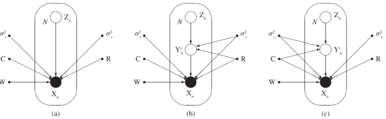
Xn C σ2 c R σ2 r Zn N W (a) Xn C σ2 c R σ2 r Zn N W Yr n (b) Xn C σ2 c R σ2 r Zn N W Yc n (c)
Fig. 1. Probabilistic graphical models for BPPCA. (a) Original generative model (14). (b) Two-stage generative model (18), with row followed by column. (c) Two-stage generative model (19), with column followed by row.
Fig. 1 shows the probabilistic graphical models of BPPCA corresponding to the three ways of generating X [(14), (18), and (19)].
D. Probability Distributions
In the following, we list the various probability distributions that can be obtained from the BPPCA model. Derivations can be found in Appendix VI Yr ∼Nqc,dr(0,I, r), Y r ∼Ndc,dr(0, σ 2 cI, r), Yc∼Ndc,qr(0, c,I), Y c ∼Ndc,dr(0, c, σ 2 rI), X∼Ndc,dr(W, c, r) (20) Z|Yr ∼Nqc,qr(Y r RM−r1,I, σr2Mr−1) (21) Yr|X∼Nqc,dr M−c1C(X−W), σc2M−c1, r (22) Yc|X∼Ndc,qr (X−W)RM−r1, c, σr2Mr−1 (23) wherec andr are given by (15) and
Mc=CC+σc2I; Mr =RR+σr2I. (24)
IV. MAXIMUMLIKELIHOODESTIMATION OFBPPCA In this section, we show how the BPPCA parameters are estimated from a given set of observations X = {Xn}nN=1.
From (20), the MLE of W is obviously the sample mean (1/N)nN=1Xn. As in PPCA, we assume that the data
has been centered. The MLE of the remaining parameters, θ = (C, σc2,R, σr2), can be obtained by maximizing the (incomplete-data) log likelihood of the BPPCA model, which is, up to a constant L(θ|X)= −1 2 N n=1 {drln|c| +dcln|r| +tr −1 c Xn−r1Xn . (25) Due to the bilinear nature of BPPCA, it is natural to develop iterative procedures for the maximization ofL. As in PPCA, it will be seen that the parameter estimation here can be easily performed by either including the latent variables (i.e., missing data) or not. Specifically, we will first present in Section IV-A a procedure based on the conditional maximization (CM) algorithm [28], which does not require the inclusion of latent variables. Then, in Section IV-B, an EM-type algorithm, which involves latent variables, will be proposed.
A. CM Algorithm
The CM algorithm is a special case of the coordinate ascent algorithm in the optimization literature [29], where the objective function [which is the incomplete-data log likelihood L (25) here] is maximized with respect to a subset of the variables at each iteration. In the following, we divide the parameters into two subsets,{C, σc2}and{R, σr2}.
1) CM-Step 1: We maximizeLwith respect to C andσc2, with{R, σr2}fixed. Equation (25) is then reduced to
Lc C, σc2|X = −N dr 2 ln|c| +tr −1 c Sc (26) where Sc = 1 N dr N n=1 Xnr−1Xn (27) = 1 N dr N n=1 dr i=1 xni−r1xni
is the sample covariance matrix of the columns of Xn’s.
Note that (26) is similar to (6). Hence, using the same derivation as in Section II-C, we obtain
C=Uc c−σc2I 1 2 Vc (28) σ2 c = 1 dc−qc dc i=qc+1 λci (29)
where Uc,Vc, and c are defined similarly as their
counterparts in Section II-C (i.e., Vc is an arbitrary
orthogonal matrix, Uc = [uc1, . . . ,ucqc] and c = diag(λc1, . . . , λcqc), with {uci}
dc
i=1,{λci}
dc
i=1 (λc1 ≥
λc2 ≥ · · · ≥ λcdc) being the eigenvectors and eigen-values of Sc).
2) CM-step 2: We maximizeL with respect to R andσr2,
with {C, σc2} fixed. This maximization is analogous to that in CM-step 1. Define the sample covariance matrix of the rows of Xn’s as Sr = 1 N dc N n=1X nc−1Xn. (30) Then (25) becomes Lr(θ|X)= − N dc 2 ln|r| +tr −1 r Sr
Algorithm 1 CM algorithm for BPPCA
Input: DataX and (random) initialization of R, σ2
r.
1: Compute the sample meanX and center the data as X¯ n ←
Xn− ¯X.
2: repeat
3: CM-step 1: Compute Sc via (27). Update C andσc2 via
(28) and (29).
4: CM-step 2: Compute Sr via (30). Update R andσr2 via
(31) and (32).
5: until change of Lis smaller than a threshold.
Output: (C,R, σc2, σr2).
and the optimal solution is
R=Ur r −σr2I 1 2 Vr (31) σ2 r = 1 dr −qr d i=qr+1 λri (32)
where Ur,Vr, and r are defined similarly as in
CM-step 1 (but based on (30)).
The whole CM algorithm is shown in Algorithm 1. Since the CM algorithm is based on coordinate descent, both CM-steps 1 and 2 will increase the log likelihoodL. Moreover, it can be easily seen that the so-called “space filling” condition4 is satisfied here. Hence, the CM algorithm is guaranteed to converge to a stationary point ofLunder the same convergence conditions as for standard EM [30].
1) Remarks: Note that the two CM-steps are equivalent to performing PPCA. Recall from (20) that
Xn ∼ Ndc,dr(0, c, r). In CM-step 1, with R and σ2
r fixed, Xnr−1/2 ∼ Ndc,dr(0, c,I) and its columns {xnir−1/2}i=1,...,dr,n=1,...,N are i.i.d. and follow Ndc(0, c). The covariance of these N dr transformed observations is
Sc in (27). Thus, CM-step 1 performs PPCA on these
transformed observations. Similarly, CM-step 2 performs PPCA on the transformed rows of Xn (N dc i.i.d. transformed
observations). On the other hand, PSOPCA fails to provide such an important connection.
Moreover, similar to PPCA, (28) and (31) show that the MLE of the factor loading matrices C and R are principal subspaces of the column and row covariance matrices Sc and
Sr, respectively (up to scaling and rotation).
Comparing (11), (12), (27), and (30), we can find that Gc
and Gr are different from Sc and Sr. Therefore, the principal
components by BPPCA and GLRAM are in general different.
2) Computational Complexity: The most expensive
compu-tations are on the formations of Scin (27), Sr in (30) and their
eigen-decompositions. Using −1 c = 1 σ2 c (I−CM−c1C). (33)
4Loosely speaking, this means unconstrained maximization is allowed over the whole parameter space [30].
Sc can be computed as Sc= 1 N drσc2 n XnXn−(XnC)M−c1(XnC) . Computing XnXn and XnC take O(dc2dr) and O(dcdrqc)
time, respectively. Given XnC, computing(XnC)Mc−1(XnC)
takes O(dc2qc) time. Let t be the number of CM
itera-tions. The total cost of forming all the Sc’s is O(N dc2dr)+ O(N t(dcdrqc + dc2qc)). Similarly, the cost of computing
all the Sr’s is O(N dr2dc)+O(N t(drdcqr +dr2qr)).
Eigen-decompositions of Sc and Sr take O(tdc3) and O(tdr3),
respectively. Hence, the total cost is O(N[dcdr(dc+dr)])+ O(N t[(dc+dr)2max(qc,qr)])+O(t[dc3+dr3]). This is similar
to that of GLRAM [11] except for the extra first term.
B. Alternating Expectation Conditional Maximization (AECM) Algorithm
In this section, we fit the BPPCA model by an EM-type algorithm called AECM algorithm [31]. Compared to the CM algorithm developed in Section IV-A, EM-type algorithms often enjoy lower computation complexity [14], though their convergence can be slower due to the inclusion of missing information [15].
The AECM algorithm is a flexible and powerful general-ization of the standard EM [31]. It is well-known that EM performs an E-step to obtain the so-called Q function followed by a M-step to maximize Q with respect to all parameters. In some cases, the M-step in EM is difficult to solve while it is possible to sequentially and conditionally maximize Q (CMQ) with respect to subsets of parameters. This yields the ECM algorithm [30] that replaces the M-step by a sequence of CMQ steps. In some cases, instead of maximizing Q, some CMQ steps can be performed through less data augmentation with the advantage of faster convergence. This leads to the AECM algorithm that replaces the E-step by several E-steps. The salient feature of AECM is that the augmented complete data is allowed to vary between E-steps yet convergence is guaranteed [31]. A specific application of ECM and AECM to mixtures of factor analyzers can be found in [32].
The AECM algorithm for BPPCA consists of two cycles, each with its own E-step and CM-step. As in Section IV-A, we divide the parameters into the two subsets θ1 =(C, σc2)
andθ2=(R, σr2).
1) In cycle 1, its E-step treats (X,Yr)= {Xn,Yrn}nN=1 as the complete data, which is then maximized with respect toθ1 (givenθ2) in its CM-step.
E-Step: The complete data log likelihood is
Lcom,c(θ1|X,Yr)= N n=1 lnp(Xn|Yrn)p(Yrn) . Givenθ=(θ1,θ2), we compute the expectedLcom,c(up
to a constant) with respect to the distribution p(Yr|X,θ)
Qc(θ1)= − 1 2 N n=1 drdclnσc2 +σ−2 c tr{E[(Xn−CYrn)r−1(Xn−CYrn)|Xn]} .
From (22), it is easy to obtain the required expectations
E[Yrn|Xn] =M−c1CXn (34)
and
E[Yrnr−1Yrn|Xn]
=drσc2Mc−1+E[Yrn|Xn]r−1E[Yrn|Xn]. (35) CM-Step: Givenθ2, we maximize Qcwith respect toθ1 and obtain C= N n=1 Xnr−1E[Yrn|Xn] · N n=1 E[Yrnr−1Yrn|Xn] −1 (36) σ2 c = 1 N drdc trN n=1Xn −1 r Xn −Xnr−1E[Yrn|Xn]C . (37)
2) In cycle 2, its E-step treats(Xn,Ync)= {Xn,Ycn}Nn=1 as the complete data, which is then maximized with respect toθ2 (givenθ1) in its CM-step.
E-Step: The complete data log likelihood is
Lcom,r(θ2|X,Yc)= N n=1 ln{pXn|Ycn p(Ycn)}.
Given the updatedθ1, we compute the expectedLcom,r
with respect to the distribution p(Yc|X,θ˜1,θ2), up to a
constant, as Qr(θ2)= − 1 2 N n=1 drdclnσr2+ σ−2 r tr{E[(Xn−YcR)−c1(Xn−YcR)|Xn]} . From (23), the required expectations can be obtained as
E[Ycn|Xn] =XnRMr−1 (38) and E[Yncc−1Ync|Xn] =dcσr2M− 1 r +E[Y c n|Xn]c−1E[Y c n|Xn]. (39) CM-Step: Givenθ˜1, we maximize Qr with respect toθ2 and obtain R=N n=1X n− 1 c E[Y c n|Xn] ·N n=1E[Y c n− 1 c Y c n|Xn] −1 (40) σ2 r = 1 N drdc trN n=1X nc−1Xn −Xnc−1E[Ycn|Xn]R . (41)
The whole algorithm is summarized in Algorithm 2. It can be observed that cycles 1 and 2 are guaranteed to increase the log likelihoodLof BPPCA. Under standard regularity condi-tions and the space-filling condition, the AECM algorithm is also guaranteed to converge to a stationary point of L[31].
Algorithm 2 AECM algorithm for BPPCA
Input: DataX and (random) initialization of(C,R, σ2
c, σr2).
1: Compute the sample meanX and center the data as X¯ n←
Xn− ¯X.
2: repeat
3: E-step of cycle 1: Compute the conditional expectations E[Yrn|Xn]andE[Ynrr−1Yrn|Xn]via (34) and (35).
4: CM-step of cycle 1: Update C andσc2via (36) and (37). 5: E-step of cycle 2: Compute the conditional expectations
E[Ycn|Xn]andE[Yncc−1Ycn|Xn]via (38) and (39).
6: CM-step of cycle 2: Update R andσr2via (40) and (41).
7: until change ofL is smaller than a threshold.
Output:(C,R, σc2, σr2).
1) Computational Complexity: The most expensive computations are on the formations of matrices
N
n=1Xnr−1E[Yrn|Xn] in (28) and
N
n=1Xnc−1E[Ycn|Xn]
in (31). The cost of E[Yrn|Xn] is O(dcdrqc). Using
(33), computation of Xnr−1E[Yrn|Xn] can be reduced
to O(dcdr(qc + qr)). Hence, the total cost of AECM is O(N tdcdr(qc +qr)). Note that its per-iteration complexity
is typically lower than that of the CM algorithm, especially when one or both data dimensionalities (dc and dr) is high.
C. Compression and Reconstruction
In this section, we compare the compressed representations and reconstructions under PPCA [4] and the proposed BPPCA. The key difference is that the operators in PPCA are linear while those in BPPCA are bilinear.
In the following, we letθˆ be the MLE ofθ,x andˆ X be the
reconstructed values of x and X, respectively.
1) PPCA:
a) Compression: Given an observation x, we takeE[z|x]
in (9) in the low-dimensional latent space as the compressed representation.
b) Linear reconstruction: Given the compressed repre-sentationE[z|x], we can reconstructxˆ=CE[z|x]+μ
from (3). Using (9), xˆ −μ = CM−1C(x−μ). In general, CM−1C is not a projection matrix [25], except whenσ2→0.
c) Orthogonal linear reconstruction: We can also recon-struct as xˆort h =C(CC)−1ME [z|x] +μ [4]. Using
(9), we have xˆort h−μ = C(CC)−1C(x−μ), in
whichC(CC)−1C is a projection matrix [4].
2) BPPCA:
a) Compression: Similar to PPCA, we take E[Z|X] as the compressed representation. Using (21) and (22), this can be computed as
E[Z|X] =E[E[Z|Yr]|X] =Mc−1C(X−W)RMr−1
(42) where the inner expectation is with respect to the distribution p(Z|Yr)and the outer one is with respect to p(Yr|X).
b) Bilinear reconstruction: Given the compressed repre-sentationE[Z|X], we can reconstruct X from (14) as
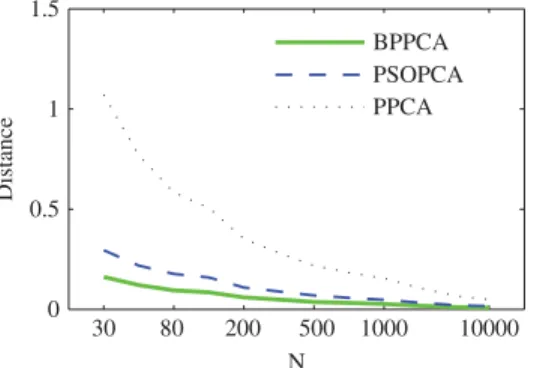
30 80 200 500 1000 10000 0 0.5 1 1.5 Distance N BPPCA PSOPCA PPCA
Fig. 2. Arc length distance between the estimated and true principal subspaces at different sample sizes.
X=CE[Z|X]R+W. Using (42), we have X−W =
CM−c1C(X−W)RM−r1R. In general, this is not a
biorthogonal projection sinceCM−c1C andRMr−1R
are not projection matrices, except when σc2 → 0
andσr2→0.
c) Biorthogonal bilinear reconstruction: We can also reconstruct X as Xort h =
C(CC)−1McE[Z|X]Mr(RR)−1R + W. Using
(42), we have Xort h − W = C(CC)−1C(X −
W)R(RR)−1R, which is a biorthogonal projection since C(CC)−1C and R(RR)−1R are projection matrices.
V. EXPERIMENTS
In this section, we perform experiments on a number of synthetic and real-world data sets. Unless otherwise stated, the CM algorithm with fast convergence (Section IV-A) is used for BPPCA. For BPPCA and GLRAM, iteration is stopped when the relative change in the objective (|1−L(t)/L(t+1)|) is smaller than a threshold tol (=10−5 in the experiments) or the number of iterations exceeds a certain maximum tmax (= 20). For PSOPCA, we use the variational EM learning algorithm in [14] for the general noise case and follow their experimental setting to set tmax=20.
A. Accuracies of the Estimators
In this experiment, we sample a 2-D synthetic data set from a 10×10-D matrix-variate normal distribution. The column and row covariance matrices have differ-ent eigenvalues (5,4.5,4,1, . . . ,1 and 10,9,8,2, . . . ,2, respectively, of which the first three are dominant), and their leading principal components are the same ([1/√2,−1/√2,0, . . . ,0], [0,0,1/√2,−1/√2, 0, . . . ,0] and[0,0,0,0,1/√2,−1/√2,0, . . . ,0]).
We compare the accuracies of the following methods in estimating the dominant principal subspace of the data.
1) BPPCA, with qc=qr =3;
2) PSOPCA [14], with qc=qr =3; and
3) PPCA [4] on the vectorized 1-D data, with
q=qcqr =9.
The subspaces of BPPCA and PSOPCA are spanned by the columns of R ⊗ C in (14) and (13), respectively.
TABLE I
NEGATIVELOG-LIKELIHOODVALUES ANDARCLENGTHDISTANCES OBTAINED FORTENDIFFERENTINITIALIZATIONS OFCM
Iteration Trial 1 2 3 4 Distance 1 76714.2 60168.4 60168.0 60168.0 0 2 71073.9 60168.2 60168.0 60168.0 7.74e–08 3 73446.2 60168.2 60168.0 60168.0 7.15e–08 4 72262.2 60168.2 60168.0 60168.0 1.00e–07 5 72716.3 60168.2 60168.0 60168.0 1.17e–07 6 72890.9 60168.2 60168.0 60168.0 1.50e–07 7 73390.6 60168.2 60168.0 60168.0 8.94e–08 8 70523.1 60168.2 60168.0 60168.0 1.10e–07 9 72355.2 60168.2 60168.0 60168.0 1.29e–07 10 72554.5 60168.2 60168.0 60168.0 1.30e–07
The performance criterion is the arc length distance between the estimated subspace and the true one [33]. Let Pˆ,P ∈ R100×9be the orthogonal bases of the two subspaces, respec-tively. The arc length between them is defined asθ2, where θ = [θ1, . . . , θ9], with{cos(θi)}9
i=1 being the singular values of PˆP. To reduce statistical variability, results for all the
methods are averaged over 50 repetitions.
Fig. 2 shows the arc length distances obtained at different sample sizes (N ). It can be observed that: 1) as N increases, the principal subspaces obtained by all three methods all converge to the true one; and 2) with limited sample size, BPPCA performs best, which is then followed by PSOPCA, and (as expected) PPCA is the worst.
B. Sensitivity to Initialization
Recall that random initialization is used in the CM and AECM algorithms (Algorithms 1 and 2). Our experience suggests that such a simple scheme works well in practice, and almost identical stationary points of the likelihood are obtained with different random initializations. To illustrate this, we report in the following an experiment on sensitive analysis, using the data set in Section V-A (with sample size N =200). The setup follows that used for the GLRAM in [11]. In the first trial for CM, R is initialized as [I,0] and σr2 as 0.01.
For the other nine trials of CM and all ten trials of AECM, the initializations are random. To measure the differences among solutions obtained with different initializations, we measure the arc length distance between the principal subspace for the solution obtained with CM’s first trial and those from the other random initializations.
Results for CM and AECM are shown in Tables I and II, respectively. As can be seen, different initializations converge to the same log-likelihood value and almost identical principal subspace (up to rotation).
C. Convergence of CM and AECM
In this experiment, we compare the convergence speeds of the CM algorithm (Section IV-A) and AECM algorithm (Section IV-B) for BPPCA. We use the same data set (with
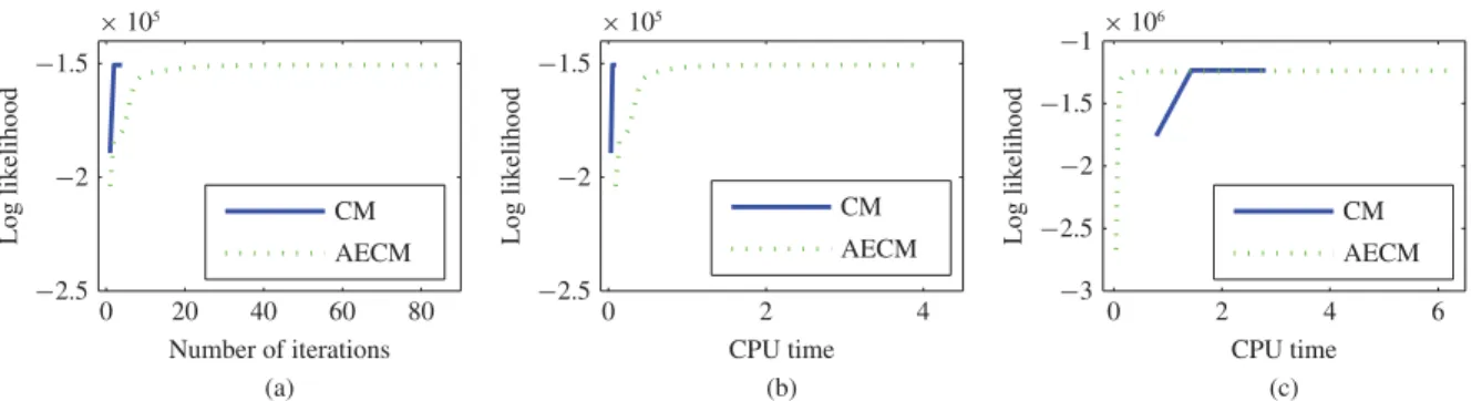
0 20 40 60 80 −2.5 −2 −1.5 × 10⁵ Lo g likelihood Number of iterations CM AECM 0 2 4 −2.5 −2 −1.5 × 10⁵ Lo g likelihood CPU time CM AECM 0 2 4 6 −3 −2.5 −2 −1.5 −1× 10 6 Lo g likelihood CPU time CM AECM (b) (c) (a)
Fig. 3. Changes in log likelihood Lfor the CM (solid) and AECM (dotted) algorithms (a) with the number of iterations on the first synthetic data set, (b) with CPU time on the first synthetic data set, and (c) with CPU time on the second high-dimensional synthetic data set.
TABLE II
NEGATIVELOG-LIKELIHOODVALUES ANDARCLENGTHDISTANCES OBTAINED FORTENDIFFERENTINITIALIZATIONS OFAECM
Iteration Trial 1 3 50 150 Distance 1 10360469819.2 72888.0 60169.5 60168.0 1.22e–07 2 10617967930.8 77084.8 60169.0 60168.0 1.46e–07 3 10912126971.6 78603.7 60172.2 60168.0 1.44e–07 4 9460828603.7 73512.5 60169.8 60168.0 1.44e–07 5 10091592873.6 74570.0 60168.5 60168.0 1.53e–07 6 11040349303.6 75792.0 60168.0 60168.0 1.49e–07 7 11432559741.1 72319.0 60168.7 60168.0 1.67e–07 8 10429865860.2 75821.6 60168.9 60168.0 1.69e–07 9 10818886067.2 73340.7 60168.3 60168.0 1.37e–07 10 10995998085.1 73546.0 60168.9 60168.0 1.59e–07
sample size N = 500) from Section V-A. Again, we fit the data with qc = qr = 3. For demonstration purpose, we set tol =10−8. Moreover, C or R are initialized randomly and σ2
c, σr2 are set to 0.01.
Fig. 3(a) plots the evolution of the log likelihood value versus the number of iterations. It can be observed that CM converges in a few iterations while AECM requires around 60 iterations to achieve comparable likelihood value. This is consistent with the theoretical result that the inclusion of missing information may yield slower convergence [15].
However, as the per-iteration complexity of AECM is lower than that of CM, it is interesting to investigate whether AECM could actually be more efficient. Fig. 3(b) plots the evolution of their log likelihood values versus CPU time. It can be observed that CM is indeed more efficient than AECM on this data set. In general, this is to be expected when the data dimensionality is not high.
When one/both of the data dimensionalities (dc and dr) is
high, AECM can become more efficient, as is demonstrated in the following experiment. We sample a data set (with sample size 50) from a 500×20-D matrix-variate normal distribution with latent dimensions qc =qr =3. Again, we fit the data
with the true latent dimensions. Fig. 3(c) plots the evolution of their log likelihood values versus CPU time. It can be observed that AECM is more efficient than CM on this high-dimensional data set.
TABLE III
METHODSUSED ON THEFACEDATASETS Method Compressed representation BPPCA E[Z|X]in (42) PSOPCA [10] E[Z|X] PPCA [4] E[z|x]in (9) GLRAM [11] UcXUr PCA [11] Uvec(X) FPCA [27] UcXUr 2-DPCA [12] XUr
D. Classification Performance on Face Data Sets
In this section, we perform face recognition experiments on two real-world image data sets.
1) XM2VTS5, which contains images for 295 individuals. Each individual has eight images taken over a period of four months. The image size is 51×55.
2) AR, which contains 126 individuals. Each individual has 26 images. As in [34], we use a subset containing 100 individuals (50 men and 50 women), and each person has 14 nonoccluded images with variations in expression and illumination. The image size is 100×100.
The data is randomly split into training and test sets, such that each class has two, three, or four training samples. The classification error rate, averaged over 20 such repetitions, will be reported. Table III lists the dimension reduction methods to be compared and their corresponding representations in the reduced-dimensional space. After the compressed rep-resentations by each method are obtained, the one-nearest-neighbor classifier is then used to obtain the error rates. For all these methods, all possible dimensionalities of the compressed representation are tried and with the best results reported.
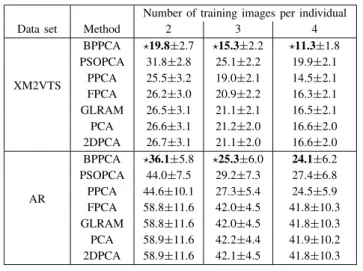
Table IV shows the error rates obtained by the various methods. The following can be seen.
1) BPPCA and PPCA substantially outperforms GLRAM, PCA and FPCA.
2) BPPCA is better than PPCA, and this can be attributed to the use of the underlying 2-D data structure. 3) BPPCA is significantly better than PSOPCA. This
indi-cates that the features obtained by BPPCA are signifi-cantly superior than those by PSOPCA.
TABLE IV
AVERAGEDERRORRATES(MEAN±STD %) OBTAINED BY THEVARIOUS METHODS ON THEFACEDATASETS. THEMETHODTHAT IS STATISTICALLYSIGNIFICANTLYBETTER(WITH A P-VALUE OF0.05
USING THETWO-SAMPLEONE-TAILEDt-TEST) THAN THEOTHER METHODS ISMARKED
Number of training images per individual
Data set Method 2 3 4
XM2VTS BPPCA 19.8±2.7 15.3±2.2 11.3±1.8 PSOPCA 31.8±2.8 25.1±2.2 19.9±2.1 PPCA 25.5±3.2 19.0±2.1 14.5±2.1 FPCA 26.2±3.0 20.9±2.2 16.3±2.1 GLRAM 26.5±3.1 21.1±2.1 16.5±2.1 PCA 26.6±3.1 21.2±2.0 16.6±2.0 2DPCA 26.7±3.1 21.1±2.0 16.6±2.0 AR BPPCA 36.1±5.8 25.3±6.0 24.1±6.2 PSOPCA 44.0±7.5 29.2±7.3 27.4±6.8 PPCA 44.6±10.1 27.3±5.4 24.5±5.9 FPCA 58.8±11.6 42.0±4.5 41.8±10.3 GLRAM 58.8±11.6 42.0±4.5 41.8±10.3 PCA 58.9±11.6 42.2±4.4 41.9±10.2 2DPCA 58.9±11.6 42.1±4.5 41.8±10.3 TABLE V
AVERAGEDERRORRATES(MEAN±STD %) OBTAINED BYBPPCAAND PPCAON THEIRIS DATASET. THEMETHODTHAT ISSTATISTICALLY
SIGNIFICANTLYBETTER(WITH Ap-VALUE OF0.05 USING THE TWO-SAMPLEONE-TAILEDt-TEST) THAN THEOTHERMETHOD IS
MARKED
Number of training samples per class
Method 5 15 25 35
BPPCA 5.2±2.2 3.5±1.1 3.2±1.2 3.2±1.8 PPCA 9.4±3.0 7.1±2.1 5.6±1.8 4.3±2.9
E. Performance on Data With Nonseparable Covariance
Recall that BPPCA relies on the assumption of separable covariance (Section III-B). For low-dimensional data, Lu and Zimmerman [23] proposed a likelihood ratio test for separabil-ity. However, for high-dimensional data sets such as those used in Section V-D, this test is impractical as the data covariance matrix becomes singular [35].
To study how nonseparability affects BPPCA, we will examine its performance on the classical iris data set, which is known to have a nonseparable covariance structure [23]. The iris data set has four variables: sepal length, sepal width, petal length, and petal width. In [23], they considered the two crossing factors: “plant part” (sepal or petal) and “physical dimension” (length or width). Using the likelihood ratio test in [23], it is shown that these two factors are not separable.
Table V compares the error rates for BPPCA and PPCA, using the one-nearest-neighbor classifier as in Section V-D. As can be seen, even though BPPCA relies on the separable covariance assumption, it is still significantly better than PPCA (which uses a nonrestrictive covariance). The difference is especially prominent on small training sets. This thus supports the observation in Section III-B that separability can trade bias for lower variance, leading to better generalization even on data sets with nonseparable covariance structure.
VI. CONCLUSION
In this paper, we proposed a bilinear probabilistic model called BPPCA for probabilistic dimension reduction on 2-D data. This signals a breakthrough from the classical 1-D latent variable model to the 2-D case. We developed two maximum likelihood estimation algorithms for BPPCA, one is based on CM while the other is based on AECM. The CM algorithm has faster convergence but higher per-iteration complexity, while the AECM algorithm has slower convergence but scales better on high-dimensional data. Similar to PPCA, we showed that the MLE of the BPPCA parameters (C and R) are principal subspaces of the column and row covariance matrices (up to scaling and rotation). In contrast, PSOPCA fails to provide such an important connection. Moreover, empirical results on synthetic data and real-world data sets demonstrate the usefulness of BPPCA over existing methods.
Nowadays, many real-world data sets are in the form of 3-D or even higher-order tensor [36]. For example, color images and grayscale video sequences can be regarded as 3-D data, while color video sequence can be regarded as 4-D. Recently, GLRAM has been extended to MPCA for the handling of tensor data [37]. In the future, we will also consider extending BPPCA, and the accompanying CM and AECM algorithms, along this direction.
APPENDIXA
MATRIX-VARIATENORMALDISTRIBUTION
The matrix-variate normal distribution is a normal distri-bution with separable covariance matrix (17) [38]. It is a generalization for the multivariate normal distribution in 1-D. Formally, it is defined as follows.
Definition 1: A random matrix X∈ Rdc×dr is said to fol-low matrix-variate normal, denoted Ndc,dr(W, c, r), with mean matrix W, column covariance matrix c ∈ Rdc×dc
and row covariance matrix r ∈ Rdr×dr, if vec(X) ∼
Ndc×dr(vec(W), r ⊗c). The pdf of X is given by
p(X)=(2π)−12drdc| c|− 1 2dr| r|− 1 2dc etr −1 2 −1 c (X−W)− 1 r (X−W) (43) where etr(·)=exp(tr(·)).
The pdf (43) of the matrix-variate normal is obtained by rewriting the pdf of vec(X) in vector form into the equivalent matrix form. If dr =1 or dc =1, the matrix-variate normal
degenerates to multivariate normal.
APPENDIXB
ROTATION ANDSCALINGINDETERMINACIES OFBPPCA The BPPCA model is unique up to the following transfor-mations.
1) Orthogonal rotations of the factor loading matrices, latent matrix, column and row noise matrices: For any orthogonal matrices Vc∈Rqc×qc and Vr ∈Rqr×qr, it is
easy to see that
CZR+W+Cr +cR+
=(CVc)(VcZVr)(VrR)+W+(CVc)(Vcr)
+(cVr)(VrR)+.
As a subspace learning method, we are interested in the subspaces spanned by the columns of C and R and hence this rotation indeterminacy is not a matter of concern. 2) Scaling of the column and row factor loading matrices.
By multiplying (C, σc) by a positive constant a and
(R, σr)by a−1 simultaneously, it is easy to see that
CZR+W+Cr +cR+
=aCZRa−1+W+aCra−1+acRa−1+aa−1.
This is not a problem as we are usually interested in: 1) the Kronecker product of the column and row para-meters (instead of either one of them); and 2) the column and row principal subspaces, and the variance ratios contained in these subspaces. For 1), clearly, the effect of scaling can be eliminated. For 2), the scaling effect is also eliminated as follows. It can be seen from (30) that the change C → aC and σc2 → aσ2
c leads to Sr → a−1Sr and hence its eigenvalues
λri→a−1λri,i =1, . . . ,dr. Consequently, Ur remains
unchanged, r → a−1r,R → a−1R in (31) and
σ2
r →a−1σr2in (32). Thus, the row principal subspace
spanned by Ur is unchanged and the variance ratio
qr i=1a− 1λ ri/ dr i=1a− 1λ ri is unchanged as well. A
similar conclusion can be drawn for the column principal subspace and its variance ratio. Thus, the scaling effect is eliminated.
APPENDIXC
DERIVATIONS FOR THEPROBABILITYDISTRIBUTIONS INSECTIONIII-D
From (18) and (43), the probability density of Yr given Z
can be obtained as p(Yr|Z)=(2πσr2)− 1 2drqc etr −1 2(Y r − ZR)σr−2(Yr−ZR) (44) and the prior density of the latent matrix Z is
p(Z)=(2π)−12qrqcetr
−1 2ZZ
. (45)
From (44) and (45), we have the marginal density of Yr
p(Yr)= p(Yr|Z)p(Z)dZ =(2π)−12drqcetr −1 2Y r−1 r Yr (46) where r is given by (15). Using the Bayes’ rule, the
conditional density of Z given Yr is
p(Z|Yr)=(2π)−12qrqc etr −1 2(Z−Y rRM−1 r )σr−2Mr(Z−YrRM−r1)
where Mr is given by (24). Similarly, from (18) and (43), the
conditional density of Yr givenc is p(Yr|c)=(2πσc2σr2)− 1 2drdc etr −1 2σ −2 c (Yr−cR)σr−2(Yr−cR) (47) and the prior distribution of the noise matrixc is
p(c)=(2πσc2)− 1 2qrdcetr −1 2σ −2 c cc . (48)
Using (47) and (48), we obtain
p(Yr)= p(Yr|c)p(c)dc =(2πσc2)−12drdc| r|− 1 2dcetr −1 2σ −2 c Y r r−1Y r . (49) Substituting Yr=X−CYr−W into (49) and using (46), we
have p(X)= p(X|Yr)p(Yr)dYr =(2π)−12drdc| c|− 1 2dr| r|− 1 2dc etr −1 2 −1 c (X−W)r−1(X−W)
wherer is given by (15), and the conditional density of Yr
given X is p(Yr|X)=(2π)−12drqc etr −1 2σ −2 c Mc(Yr −M−c1CX)r−1(Yr−M−c1CX) where Mc is given by (24). REFERENCES
[1] C. M. Bishop, Pattern Recognition and Machine Learning. New York: Springer-Verlag, 2006.
[2] K. Zhang and J. T. Kwok, “Clustered Nyström method for large scale manifold learning and dimension reduction,” IEEE Trans. Neural Netw., vol. 21, no. 10, pp. 1576–1587, Oct. 2010.
[3] S. Yu, “Advanced probabilistic models for clustering and projection,” Ph.D. dissertation, Faculty Math. Comput. Sci. Statist., Univ. Munich, Munich, Germany, 2006.
[4] M. E. Tipping and C. M. Bishop, “Mixtures of probabilistic principal component analysers,” Neural Comput., vol. 11, no. 2, pp. 443–482, 1999.
[5] D. J. Bartholomew, Latent Variable Models and Factor Analysis, 1st ed. New York: Oxford Univ. Press, 1987.
[6] J. H. Zhao and Q. Jiang, “Probabilistic PCA for t distributions,”
Neurocomputing, vol. 69, nos. 16–18, pp. 2217–2226, 2006.
[7] I. T. Jolliffe, Principal Component Analysis, 2nd ed. New York: Springer-Verlag, 2002.
[8] B. Moghaddam and A. Pentland, “Probabilistic visual learning for object representation,” IEEE Trans. Pattern Anal. Mach. Intell., vol. 19, no. 7, pp. 696–710, Jul. 1997.
[9] J. Ye, R. Janardan, and Q. Li, “GPCA: An efficient dimension reduction scheme for image compression and retrieval,” in Proc. 10th ACM Int.
Conf. Knowl. Discov. Data Min., Seattle, WA, Aug. 2004, pp. 354–363.
[10] X. Xie, S. Yan, J. Kwok, and T. Huang, “Matrix-variate factor analysis and its applications,” IEEE Trans. Neural Netw., vol. 19, no. 10, pp. 1821–1826, Oct. 2008.
[11] J. Ye, “Generalized low rank approximations of matrices,” Mach. Learn., vol. 61, nos. 1–3, pp. 167–191, 2005.
[12] J. Yang, D. Zhang, A. F. Frangi, and J. Yang, “2-D PCA: A new approach to appearance-based face representation and recognition,” IEEE Trans.