Traffic Signal Consensus Control

Portland State University Portland State University

PDXScholar

PDXScholar

TREC Final Reports Transportation Research and Education Center _(TREC)

4-2019

Traffic Signal Consensus Control

Traffic Signal Consensus Control

Portland State University, [email protected]

Follow this and additional works at: https://pdxscholar.library.pdx.edu/trec_reports

Part of the Control Theory Commons, Transportation Commons, and the Urban Studies Commons

Let us know how access to this document benefits you.

Recommended Citation

Lafferriere, Gerardo. Traffic Signal Consensus Control. NITC-RR-1165. Portland, OR: Transportation Research and Education Center (TREC), 2019. https://doi.org/10.15760/trec.213

This Report is brought to you for free and open access. It has been accepted for inclusion in TREC Final Reports by an authorized administrator of PDXScholar. For more information, please contact [email protected].

Traffic Signal Consensus Control

FINAL REPORT

NITC-RR-1165 April 2019

NITC is a U.S. Department of Transportation national university transportation center.

TRAFFIC SIGNAL CONSENSUS CONTROL

Final Report

NITC-RR-1165

by

Gerardo Lafferriere, http://orcid.org/0000-0003-0915-5976

Portland State University

for

National Institute for Transportation and Communities (NITC) P.O. Box 751

Portland, OR 97207

i Technical Report Documentation Page

1. Report No. 2. Government Accession No. 3. Recipient’s Catalog No. NITC-RR-1165

4. Title and Subtitle 5. Report Date

April 2019 Traffic Signal Consensus Control

6. Performing Organization Code

7. Author(s) 8. Performing Organization Report No.

Gerardo Lafferriere

9. Performing Organization Name and Address 10. Work Unit No. (TRAIS)

11. Contract or Grant No.

12. Sponsoring Agency Name and Address 13. Type of Report and Period Covered

National Institute for Transportation and Communities (NITC) 14. Sponsoring Agency Code P.O. Box 751

Portland, OR 97207 15. Supplementary Notes

16. Abstract

We introduce a model for traffic signal management based on network consensus control principles. The underlying principle in a consensus approach is that traffic signal cycles are adjusted in a distributed way so as to achieve desirable ratios of queue lengths throughout the street network. This approach tends to reduce traffic congestion due to queue saturation at any particular city block and it appears less susceptible to congestion due to unexpected traffic loads on the street grid. We developed simulation tools based on the MATLAB computing environment to analyze the use of the mathematical consensus approach to manage the signal control on an urban street network.

17. Key Words 18. Distribution Statement

Traffic signal control, network control, consensus No restrictions. Copies available from NITC: www.nitc-utc.net

19. Security Classification (of this report) 20. Security Classification (of this page) 21. No. of Pages 22. Price

ii

ACKNOWLEDGEMENTS

Gerardo Lafferriere would like to acknowledge partial support from the National Institute for Transportation and Communities (NITC; grant number 1165) a U.S. DOT University

Transportation Center, and the National Science Foundation (NSF; Grant number BCS-123456).

DISCLAIMER

The contents of this report reflect the views of the author, who is solely responsible for the facts and the accuracy of the material and information presented herein. This document is

disseminated under the sponsorship of the U.S. Department of Transportation University Transportation Centers Program in the interest of information exchange. The U.S. Government assumes no liability for the contents or use thereof. The contents do not necessarily reflect the official views of the U.S. Government. This report does not constitute a standard, specification, or regulation.

RECOMMENDED CITATION

Lafferriere, Gerardo. Traffic Signal Consensus Control. NITC-RR-1165. Portland, OR: Transportation Research and Education Center (TREC), 2019.

iii TABLE OF CONTENTS

EXECUTIVE SUMMARY ... 1

1.0 INTRODUCTION... 2

1.1 MATHEMATICAL MODEL ... 2

1.1.1 General Mathematical Setting ... 3

1.1.2 An Illustrative Example ... 4

1.1.3 Equations... 5

2.0 SIMULATION TOOLS AND FEATURES ... 7

2.1 TOOL DESCRIPTION ... 7 3.0 SIMULATION RESULTS ... 10 3.1 SETUP ... 10 3.2 RESULTS ... 10 3.3 FURTHER CONSIDERATIONS ... 13 4.0 REFERENCES ... 15

LIST OF FIGURES

Figure 2.1: The GUI for tlcc23.m. The long, numbered rectangles represent the car queues. The triangles are the corresponding traffic signals and point in the direction of traffic flow. In each block, one lane is a turning lane. For example, queues 2 and 14 correspond to turning lanes, right turn and left turn, respectively. ... 7

Figure 2.2: Screenshot displaying the evolution of both protocols: consensus (top), proportional (bottom). Queue lengths are notably different. ... 9

Figure 3.1: Two screenshots of the same runs corresponding to the two protocols: consensus (top), proportional (bottom). The light-colored queues indicate congestion. To simplify the display, we use the lighter color to indicate that true lengths exceed those displayed. ... 11

Figure 3.2: Analysis of queue lengths: consensus protocol (left) vs proportional protocol (right). Top plots show all queues over the duration of the run. Second row shows the standard deviation of the queue lengths: the proportional protocol shows a wider variation of lengths. The third row shows the mean queue lengths: the consensus protocol maintains shorter queues overall, reducing the load on the street grid. ... 12

Figure 3.3: Queue length evolution under different communication graphs (complete graph (solid line), one-step graph (dashed line)). Under the one-step graph queue lengths increase faster as the information flow is slower through the grid. ... 13

1

EXECUTIVE SUMMARY

We developed simulation tools to explore a new model for traffic signal management based on network consensus control principles. The model seeks to understand the evolution of the lengths of the queues at each traffic signal; that is, the number of cars waiting at the signal. Adapting existing consensus control models to traffic management required introducing a number of additional constraints that challenged the existing theory. We implemented the model in a simulation tool that allows for interactive analysis and visualization of the approach. The main contribution of the project is the simulation platform that allows for comparison between the proposed consensus approach and a standard traffic signal control protocol. The main features of the mathematical model and the simulation tools are explained and illustrated in the report. The complete open source for the code is available in the online depository. The code is in the form of MATLAB files with extensive comments explaining the various parts of the model. The tool has an intuitive graphical user interface (GUI) which facilitates exploration of the many features. Simulation runs may be saved at any time of the run in a standard MATLAB file format. The same simulation tool may be used to load and rerun previous experiments. Alternatively, the data can be explored offline with other MATLAB scripts provided.

2

1.0

INTRODUCTION

Congestion in the urban areas has been increasing with significant economic and social costs. According to the 2015 Urban Mobility Report, the total additional cost of congestion was $160 billion (Texas Transportation Institute, 2015). This problem will only be exacerbated in the future with more and more of the population moving to urban areas. Traffic signals represent a significant bottleneck for congestion management. There is a need to develop new traffic control strategies which exploit new developments in communication, sensing and intelligent

infrastructure systems. Several researchers have developed strategies for decentralized and partially decentralized decision signal optimization such as Split Cycle Offset Optimization Technique (Hunt, Robertson, Bretherton, & Winton, 1981); SCATS - Sydney Co-ordinated Adaptive Traffic System (Lowrie, 1990); RHODES - Real Time Hierarchical Optimized

Distributed Effective System (Mirchandani & Wang, 2005); and OPAC - Optimized Policies for Adaptive Control (Gartner, 2001). However, these strategies are limited in the network level congestion management (Papageorgiou, Diakaki, Dinopoulou, Kotsialos, & Wang, 2003). Here we propose a new approach to urban traffic signal control based on network consensus control theory which is computationally efficient, responsive to local congestion, and at the same time has the potential for congestion management at the network level.

We have implemented a consensus approach in a MATLAB simulation module to explore the potential benefits to traffic flow.

1.1

MATHEMATICAL MODEL

The model seeks to understand the evolution of the lengths of the queues at each traffic signal; that is, the number of cars waiting at the traffic signal. We use a discrete time model. Essentially, we quantify time and study the evolution as this time unit is incremented. The signals’ cycle-time will be measured in multiples of this basic time unit. The basic time unit used corresponds to two seconds, which we take as the average time for a vehicle to move through the intersection. This basic time unit can be adjusted easily in the main code.

A consensus/agreement protocol aims to achieve a common value of the “state” variables via a distributed algorithm in which values of each state variable are updated based on the values of its “neighbors” in a communication graph. More precisely, a networked control system consists of a number of dynamical systems called “agents” which are linked via a communication or sensor graph. The state of each agent evolves according to both its own dynamics and the dynamics of its neighbors in the communication graph. In a consensus protocol, the neighbors’ influences come through a weighted average of their current states. The basic theory guarantees that, under minimal connectivity conditions on the communication graph, the states converge asymptotically to a common value. This “consensus” value is achieved using only local computations. There is a balance between computational requirements and robustness of the network: fewer edges in the communication graph results in more localized computations requiring less computing power at each node, and more edges lead to more robust behavior in the presence of uncertainty and disruptions.

3

The theory of consensus or agreement protocols for networked control systems has been developed extensively over the last decade. This subfield of mathematical control theory has been used to model a number of situations where a distributed calculation approach achieves global optimal objectives or when emergent behaviors result from distributed decision making. Some examples of application include formation control of autonomous vehicles (Lafferriere & Mathia, 2008) (Olfati-Saber, Fax, & Murray, 2007) (Veerman, Lafferriere, Caughman, &

Williams, 2005) (Williams, Lafferriere, & Veerman, 2005) (Lafferriere, Williams, Caughman, & Veerman, 2005) (Lafferriere, Caughman, & Williams, 2004); distributed estimation in sensor networks (Das & Mesbahi, 2009) (Ren, Beard, & Atkins, 2007); and vulnerability of networked synchronization processes (Dhal, Lafferriere, & Caughman, 2016)(see also the books (Mesbahi & Egerstedt, 2010), (Bullo, Cortés, & Martínez, 2009), and (Ren & Beard, 2008) for many other references). In these models, autonomous “agents” adjust their state relying on local information so as to achieve consensus on a global objective.

In the context of urban traffic, queue lengths play the role of agents and the goal is to achieve a prescribed ratio of queue lengths: for example, we may desire all queues to have the same length and, thus, effectively balance the load on all roads. Alternatively, the goal could be to achieve a desired “deviation” from a nominal set of lengths determined from historical data. These deviations could be used to indirectly redistribute loads on the city grid based on evolving situations, such as traffic accidents or deteriorating road conditions.

The basic mathematical set up resulting from a consensus approach must be modified and

adapted to handle all the features inherent in modeling urban traffic: traffic flow theory for traffic propagation, car delays, lane choice, congestion, etc. At present, the existing mathematical consensus theory does not extend to include all such additional constraints.

We developed simulation tools to explore how to include relevant traffic constraints in a consensus protocol and to understand how this approach affects overall traffic behavior.

1.1.1

General Mathematical Setting

The process is modeled as a discrete-time dynamical system. A time step corresponds to a (small) basic unit of time. All green indications stay on for an integer multiple of this basic unit of time, so the same signal could stay green during various transition steps of the model. All signals are on the same clock.

We define three graphs. All are (generally) directed graphs and so they consist of a set of nodes (or vertices) and a set of ordered pairs of nodes (which we call edges). If the graph is undirected, allowing for bidirectional communication, that simply means that (𝑖𝑖,𝑗𝑗) is an edge if and only if (𝑗𝑗,𝑖𝑖) is an edge. The variable 𝑛𝑛 will denote the total number of queues. The 𝑛𝑛-vector 𝑦𝑦 will represent the length of all the queues. This vector 𝑦𝑦 is the state variable for the dynamical system.

1. The communication graph 𝑮𝑮_𝒐𝒐 = (𝑽𝑽(𝑮𝑮_𝒐𝒐),𝑬𝑬(𝑮𝑮_𝒐𝒐)). This refers to the digraph in 𝑛𝑛 nodes (so 𝑉𝑉 = {1, … ,𝑛𝑛}) that specifies which queues are compared at each iteration. We say that 𝑗𝑗 is an in-neighbor of 𝑖𝑖 in 𝐺𝐺_𝑜𝑜 if (𝑖𝑖,𝑗𝑗) is in 𝐸𝐸(𝐺𝐺_𝑜𝑜). We denote by 𝑁𝑁_𝑜𝑜(𝑖𝑖) the set of

in-4

neighbors of 𝑖𝑖. If 𝑗𝑗 is in 𝑁𝑁_𝑜𝑜(𝑖𝑖), then information about 𝑗𝑗 “flows” to 𝑖𝑖. Alternatively, we say that node 𝑖𝑖 uses knowledge of node 𝑗𝑗.

2. The conflict graph 𝑮𝑮_𝒄𝒄. This is an undirected graph on 𝑛𝑛 nodes. This encodes the queues that meet at an intersection and, thus, are governed by the same traffic signal. At any step of the iteration, only one of the conflicting queues can be reduced. We say two queues 𝑖𝑖,𝑗𝑗 are in conflict if (𝑖𝑖,𝑗𝑗) is an edge of this graph. We write 𝑁𝑁_𝑐𝑐(𝑖𝑖) for the set of neighbors of 𝑖𝑖.

3. The traffic flow graph 𝑮𝑮_𝒇𝒇. This is a digraph on 𝑛𝑛 nodes. This graph indicates which queues will feed into which other ones once the signal turns green for the first one. We write 𝑁𝑁_𝑓𝑓(𝑖𝑖) for the set of in-neighbors of 𝑖𝑖.

For any digraph we also say that 𝑖𝑖 is an out-neighbor of 𝑗𝑗 if 𝑗𝑗 is an in-neighbor of 𝑖𝑖. For undirected graphs every in-neighbor is also an out-neighbor and vice versa.

For each graph we define a corresponding adjacency matrix. An adjacency matrix has a 1 in entry (𝑖𝑖,𝑗𝑗) if 𝑗𝑗 is an in-neighbor of 𝑖𝑖. The matrix has zeros in all other entries.

We will denote the corresponding adjacency matrices associated to each graph above as 𝐴𝐴_𝑜𝑜, 𝐴𝐴_𝑐𝑐, and 𝐴𝐴_𝑓𝑓, respectively. Since 𝐺𝐺_𝑐𝑐 is undirected, 𝐴𝐴_𝑐𝑐 is a symmetric matrix.

1.1.2

An Illustrative Example

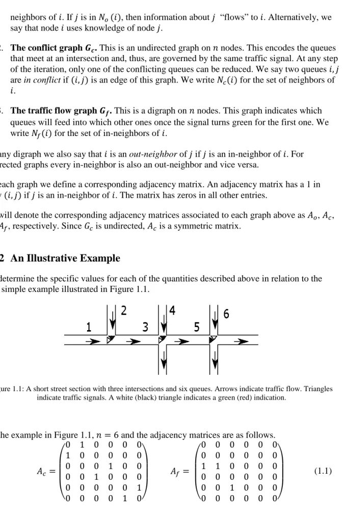
We determine the specific values for each of the quantities described above in relation to the very simple example illustrated in Figure 1.1.

Figure 1.1: A short street section with three intersections and six queues. Arrows indicate traffic flow. Triangles indicate traffic signals. A white (black) triangle indicates a green (red) indication.

For the example in Figure 1.1, 𝑛𝑛 = 6 and the adjacency matrices are as follows.

𝐴𝐴𝑐𝑐 = ⎝ ⎜ ⎜ ⎛ 0 1 0 0 0 0 1 0 0 0 0 0 0 0 0 1 0 0 0 0 1 0 0 0 0 0 0 0 0 1 0 0 0 0 1 0⎠ ⎟ ⎟ ⎞ 𝐴𝐴𝑓𝑓= ⎝ ⎜ ⎜ ⎛ 0 0 0 0 0 0 0 0 0 0 0 0 1 1 0 0 0 0 0 0 0 0 0 0 0 0 1 0 0 0 0 0 0 0 0 0⎠ ⎟ ⎟ ⎞ (1.1)

5

Notice, for example, that in the conflict matrix 𝐴𝐴_𝑐𝑐 there are 1s in entries (3,4) and (4,3) to indicate that queues 3 and 4 are governed by the same traffic signal (similarly for queues 1 and 2 and for queues 3 and 4). In 𝐴𝐴_𝑓𝑓 there is a one in entry (3,1) because cars from queue 1 flow into queue 3. A similar interpretation applies to the other entries. The communication graph 𝐺𝐺_𝑜𝑜 is, in principle, independent from the geographical arrangement of roads and queues.

For the first simulations, we coded a few standard graphs: complete, path, cycle, etc. In practice, some useful communication graphs are, in fact, related to the geographical location of the signals. For example, the one-step graph used in some of the simulations below corresponds to having the signals immediately up and down stream be “neighbors” (also referred to as a one-hop rule).

We introduce an associated Laplacian matrix to 𝐴𝐴_𝑜𝑜 as follows. For each node 𝑖𝑖 let 𝑑𝑑(𝑖𝑖) denote the number of in-neighbors of 𝑖𝑖. We call 𝑑𝑑(𝑖𝑖) the in-degree of node 𝑖𝑖. Let ∆_𝑜𝑜 denote the diagonal matrix with (∆_𝑜𝑜)_{𝑖𝑖𝑖𝑖} = 𝑑𝑑(𝑖𝑖). That is, ∆_𝑜𝑜 is the diagonal matrix of in-degrees. We now define the Laplacian matrix, 𝐿𝐿, associated to 𝐴𝐴_𝑜𝑜 as

𝐿𝐿 = ∆𝑜𝑜 − 𝐴𝐴𝑜𝑜. (1.2)

Note that 𝑑𝑑(𝑖𝑖) is the sum of the 𝑖𝑖-th row of the matrix 𝐴𝐴_𝑜𝑜. It follows that the sum of the rows of 𝐿𝐿 are all zero. Put another way, if 1 is the column vector with all 1's, then 𝐿𝐿𝟏𝟏= 0. This says, in particular, that 0 is an eigenvalue of 𝐿𝐿 and that 1 is a corresponding eigenvector. For a connected graph, the number 0 is always a simple eigenvalue and the size of the smallest non-zero

eigenvalue determines the stability properties of the network, for example, the rate of convergence to a consensus value.

1.1.3

Equations

To describe the equations and to account for appropriate truncations (since queues must have nonnegative length) we need some additional definitions. The function 𝜎𝜎:ℝ𝑛𝑛 →{0,1}nis given as follows. For 𝑖𝑖= 1, … ,𝑛𝑛, 𝜎𝜎(𝑦𝑦)_𝑖𝑖 =� 1, 𝑖𝑖 𝑦𝑦𝑖𝑖 > max_{𝑗𝑗∈𝑁𝑁} 𝑐𝑐(𝑖𝑖)𝑦𝑦𝑗𝑗; 1, 𝑖𝑖 𝑦𝑦𝑖𝑖 = max_{𝑗𝑗∈𝑁𝑁} 𝑐𝑐(𝑖𝑖)𝑦𝑦𝑗𝑗 𝑎𝑎 𝑖𝑖 < min𝑗𝑗∈𝑁𝑁𝑐𝑐(𝑖𝑖)𝑗𝑗; 0, 𝑜𝑜𝑜𝑜ℎ𝑒𝑒𝑒𝑒𝑒𝑒 𝑒𝑒𝑒𝑒. 𝑓𝑓 𝑓𝑓 𝑛𝑛𝑑𝑑 𝑖𝑖 (1.3)

This function works as a decision variable to determine which queue at a traffic signal gets the green indication. Next, we introduce a few parameter vectors.

• _{𝒓𝒓𝒐𝒐𝒐𝒐𝒐𝒐}. This represents the number of cars in each queue that gets through the signal once it turns green. More precisely, during each time unit while the indication is green for queue 𝑖𝑖, the queue will be shortened by 𝑒𝑒_{𝑜𝑜𝑜𝑜𝑜𝑜}(𝑖𝑖) vehicles. This does not account for startup delays for vehicles to move, but this is one of the simplifications we used in order to

6

focus on the impact of the main signal-cycle schedules. We explain below how we introduced additional constraints to account for some delays in the car movements.

• _{𝒓𝒓𝒊𝒊𝒊𝒊}. This represents the input rate of vehicles to queues on the peripheral queues; that is, the rate at which the vehicles are entering the street grid.

The dynamic equations can now be written as a system in the following form: 𝑐𝑐 𝑜𝑜𝑜𝑜𝑜𝑜 = 𝜎𝜎�𝑦𝑦( )� ⋅ 𝑜𝑜𝑜𝑜𝑜𝑜 ⋅max(𝐿𝐿 ( ), 0) 𝑐𝑐 𝑖𝑖 = 𝐴𝐴𝑓𝑓�𝜎𝜎�𝑦𝑦( )� ⋅ 𝑜𝑜𝑜𝑜𝑜𝑜�+ 𝑖𝑖 𝑦𝑦( + 1) = max(𝑦𝑦( )− 𝑐𝑐 𝑜𝑜𝑜𝑜𝑜𝑜 +𝑐𝑐 𝑖𝑖 , 0) 𝑎𝑎𝑒𝑒𝑒𝑒 𝑜𝑜 𝑒𝑒 𝑦𝑦 𝑜𝑜 𝑎𝑎𝑒𝑒𝑒𝑒𝑛𝑛 𝑜𝑜 𝑒𝑒 𝑒𝑒𝑛𝑛 𝑜𝑜 𝑜𝑜 𝑎𝑎𝑒𝑒𝑒𝑒 𝑎𝑎𝑒𝑒𝑒𝑒𝑛𝑛 (1.4)

Here 𝑜𝑜 is the current time step and the dot stands for multiplication entry by entry. The “max” functions are there to guarantee that some quantities are nonnegative, since we can never have a negative number of vehicles in a queue. Finally, we could put it all into one system of equations to better see the overall structure.

y(t + 1) = max�y(t)− σ�y(t)� ⋅max�sgn�Ly(t)�, 0�+ Af�σ�y(t)� ⋅rout�+ rin, 0� (1.5)

While this equation accounts for the essential part of the consensus protocol, the incorporation of typical traffic constraints such as signal conflicts, car delays, and minimum green times required the introduction of additional decision variable in the computer code.

7

2.0

SIMULATION TOOLS AND FEATURES

2.1

TOOL DESCRIPTION

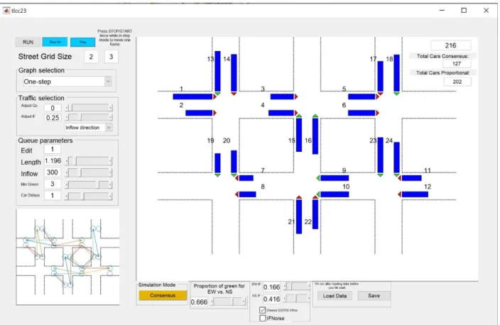
The simulation tool was built using the MATLAB computer software from MathWorks. We used the MATLAB graphical user interface development environment (GUIDE) to create a GUI which allows the user to visualize the simulation runs in an easy-to-understand environment and provide direct access to a number of simulation parameters. Some of these parameters can be modified “on the fly” while the simulation is running. The screenshot in Figure 2.1 shows the nature of the GUI.

Figure 2.1: The GUI for tlcc23.m. The long, numbered rectangles represent the car queues. The triangles are the corresponding traffic signals and point in the direction of traffic flow. In each block, one lane is a turning lane. For

example, queues 2 and 14 correspond to turning lanes, right turn and left turn, respectively.

We provide two versions of the main tool: tlcc23.m and tlcc34.m. The numbers refer to the street grid size. Users can modify two lines in the source code to create other rectangular grids. We describe below some of the tool features and explain how some additional flexibility could be added for the exploration of the consensus protocol.

1. Two protocols are implemented simultaneously: the consensus approach and a fixed pattern approach which we called proportional. In this second method, the signals turn green in a

8

fixed proportion of time at each intersection. By default, N/S streets get a green indication twice as long as the E/W streets. This proportion can be changed by the user within the GUI. As long as the inflow of cars into N/S streets and E/W streets maintain that ratio, the

proportional protocol is efficient. When those inflow rates are changed, the consensus protocol adapts and becomes more efficient in that fewer cars are held up in the grid. The user can visualize the two approaches by switching which mode to display using a push button. Both simulations run simultaneously. (For analysis purposes, the queue lengths for the consensus protocol are stored in the variable 𝑦𝑦 and those for the proportional protocol are in 𝑦𝑦_𝑓𝑓.)

2. There are two lanes on each block one for turning and one for going straight. Cars entering a block distribute into the two lanes in a 1-to-2 ratio: for every car turning, two go straight. This ratio is changeable in the code but not yet available on the GUI. It is important to note that each lane has its own dedicated signal. Under the proportional protocol both the straight lane and the turning lane traffic signals turn green (or red) simultaneously to preserve the constant green/red ratio. However, in the consensus protocol they are allowed to change independently, restricted only by the fact that vehicles cannot cross each other at an intersection. This constraint is captured in the conflict matrix mentioned earlier.

3. We built in a delay, as each signal turns green, to account for the fact that cars take some time to accelerate and get through the intersection. This is a simplification to somewhat account for some delay at start up, but it does not account for more sophisticated vehicle dynamics.

4. We also built in a minimum time for the green indications to be on (this is configurable through the GUI). While in a regular consensus protocol signals could possibly switch at every cycle, this minimum time will allow for more realistic simulations. It is natural to expect that any signal protocol should allow for some minimum number of cars (at least one) to go through during each green indication cycle.

5. The users can choose from several communication graphs pre-coded or load their own custom graph. There is an additional tool to generate custom graphs. This is separate from the main simulation tool but it is well integrated with it. The communication graph

determines which queues pass information to each other when making a decision on which signal to turn green. The simulation assumes that queue lengths are recorded or estimated from street sensors.

6. Data from a simulation run can be saved to a file. This file contains all the necessary information to repeat the simulation using the same programs. The saved files also include additional information for further analysis, such as all the relevant adjacency matrices. These files were used to analyze the particular runs offline and compare the two protocols.

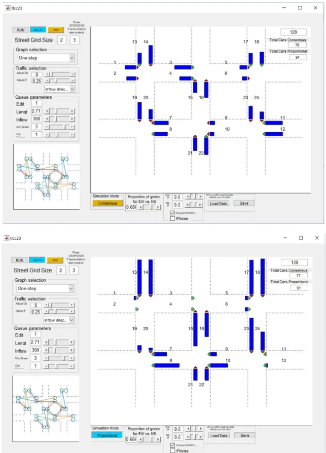
The computer screenshots displayed in Figure 2.2, show the GUI of the simulation tool. The user has direct access to a number of features mentioned above. The two images correspond to the same simulation run with the same initial values and the same parameters values, but reflect the two protocols implemented. The screenshots capture both the consensus and the proportional simulation modes.

9

Figure 2.2: Screenshot displaying the evolution of both protocols: consensus (top), proportional (bottom). Queue lengths are notably different.

10

3.0

SIMULATION RESULTS

To illustrate the use of the simulation tools, we ran a number of computers experiments to compare the impact of sudden changes in traffic flow patterns on overall congestion in the grid. We archived the results of the simulations described below in the public depository

(https://github.com/gerardolf/Traffic_Light_Code).

3.1

SETUP

The simulations illustrated below start with a random initial distribution of cars in the various queues. We set the inflow patterns (IF) to match the proportional protocol. That is, the inflow on E/W streets is twice that of the N/S streets and, correspondingly, the E/W traffic signals in the proportional protocol stay green for twice as long as the N/S signals. After some time, we significantly increase the inflow rate on the N/S access queues. During this time, we observe how the total number of vehicles in the grid increases at different rates for the two protocols. After some additional time passed, we restore the original inflow rates to examine how the load on the systems is reduced by the two protocols.

3.2

RESULTS

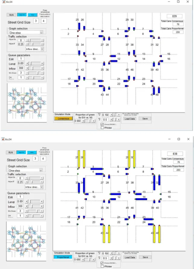
Once the inflow rates are changed, the proportional approach can no longer keep traffic flowing at a fast-enough rate. This results in significant congestion at the access streets to the grids. At the same time, traffic load is very low on many inner blocks. On the other hand, the consensus approach was able to distribute traffic more efficiently and kept the load on all streets at a comparable level. This is represented in the screen shots in Figure 3.1. As can be observed from the plots, the queues do not have identical lengths. This seems mostly due to the effect of decision variables that account for minimum green indications times and car delays. The longer we force green indications to stay on, the more we depart from a true consensus protocol. This general behavior of the queues, of staying within a small range of values, is typical of the consensus protocol and is mostly independent of the communication graph used. It should be noted that the communication graph used in this particular run is a one-step graph with rather few edges. That is, only information from neighboring traffic signals are used to decide on the adjustment. Yet, because the graph is connected, the information does propagate through the whole street network, maintaining a rather homogenous distribution of queue lengths throughout. We describe further below one feature of the simulation that does vary based on the graph used.

11

Figure 3.1: Two screenshots of the same runs corresponding to the two protocols: consensus (top), proportional (bottom). The light-colored queues indicate congestion. To simplify the display, we use the lighter color to indicate

12

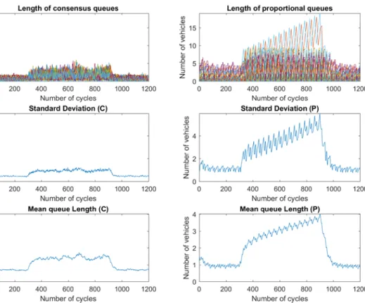
We also provide simple tools to analyze the simulation results offline (tlcc_plots.m). In Figure 3.2 we show how the queue lengths evolve under the two protocols. Not only do more cars clog the system when the proportional protocol cannot keep up, but the queue lengths have a larger variance. This makes inefficient use of the roads and creates more chances for congestion at different points.

Figure 3.2: Analysis of queue lengths: consensus protocol (left) vs proportional protocol (right). Top plots show all queues over the duration of the run. Second row shows the standard deviation of the queue lengths: the proportional protocol shows a wider variation of lengths. The third row shows the mean queue lengths: the consensus protocol

maintains shorter queues overall, reducing the load on the street grid.

As mentioned earlier another feature of the approach is the possibility of using different

communication graphs among the traffic signals. More precisely, the decisions of which signals turn green are based on comparing queue lengths between neighboring queues as determined by the communication graph. These “neighbors” do not need to be physically close, though in a couple of the graphs used they are.

This flexibility of the approach has been incorporated in the simulation tools. The users may select from a few graphs or load their own one, previously generated with another supporting tool. The graph used in the run is displayed on the lower left corner of the GUI. The one-step graph used in this particular simulation, illustrated here, corresponds to essentially a one-hop look ahead (and back); that is, queues are compared with those immediately up or down traffic

13

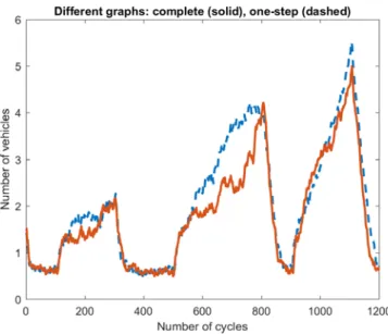
from them. That means that each signal uses information from at most four nearby queues to adjust their timing. Using richer graphs, such as the complete graph produces a different evolution of queue lengths. Figure 3.3 illustrates this by showing runs with similar parameters but different communication graphs. The average queue length appears to grow faster at times under the one-step graph. This may be a result of not being able to effectively move traffic based on information about all the queues. The information about the various queue lengths flows more slowly through the system when the communication graph has fewer edges.

Figure 3.3: Queue length evolution under different communication graphs (complete graph (solid line), one-step graph (dashed line)). Under the one-step graph queue lengths increase faster as the information flow is slower

through the grid.

Besides the main simulation tools, we also include a macro to generate arbitrary communication graphs (graphgen.m). A graph generated by this tool can then be loaded on tlcc23.m or tlcc34.m by choosing the “custom” option in the drop-down menu of the graph selection box in the GUI. We provide two examples in the files adj*.mat available in the software depository.

3.3

FURTHER CONSIDERATIONS

There are a number of issues that need exploring in more detail. We would like to establish the precise threshold that makes one traffic signal protocol better than the other on the various metrics: total number of vehicles in the system, number of congested streets, variance on queue lengths, etc. This could have very practical uses in order to implement multiple protocols based on the state of the grid at any given time.

In order to implement a protocol as closely based on the consensus approach as possible, we minimized the number of additional restrictions that may be necessary in a full implementation. While the current code includes special logic to account for minimum green times and car delays

14

as explained earlier, we have not yet implemented other features, such as maximum red indications and a separate treatment of exit queues, among others.

There are many more questions that may be investigated with the simulation tools created. With the current state of the tools and the access to the full source we expect many researchers to be able to explore the potential of the network consensus protocol.

15

4.0

REFERENCES

Bullo, F., Cortés, J., & Martínez, S. (2009). Distributed Control of Robotics Networks: A Mathematical Approach to Motion Coordination Algorithms. Princeton: Princeton University Press.

Das, A., & Mesbahi, M. (2009). Distributed parameter estimation over sensor networks. IEEE Transactions on Aerospace Systems and Electronics, 45(4), 1293—1306.

Dhal, R., Lafferriere, G., & Caughman, J. (2016). Towards a complete characterization of vulnerability of networked synchronization processes. Proc. 55th IEEE Conference on Decision and Control, (pp. 5207-5212).

Gartner, N. (2001). Optimized Policies for Adaptive Control (OPAC). Retrieved from

http://www.signalsystems.org.vt.edu/documents/Jan2001AnnualMeeting/TRB2001_Slide s_for_posting.pdf

Hunt, P., Robertson, D., Bretherton, R., & Winton, R. (1981). SCOOT—A Traffic Responsive Method of Coordinating Signals. Crowthorne, Berkshire, U.K.: Transport and Road Research Laboratory.

Lafferriere, G., & Mathia, K. (2008). Control of Formations under Persistent Disturbances. Proc. of the American Control Conference, (pp. 795--800).

Lafferriere, G., Caughman, J., & Williams, A. (2004). Graph theoretic methods in the stability of vehicle formations,., pp. 3724-3729 (2004). Proc. of the 2004 American Control Conf, (pp. 3724--3729).

Lafferriere, G., Williams, A., Caughman, J., & Veerman, J. (2005). Decentralized Control of Vehicle Formations. Systems & Control Letters, 54, 899--910.

Lowrie, P. (1990). SCATS, Sydney Co-Ordinated Adaptive Traffic System : A Traffic Responsive Method Of Controlling Urban Traffic. Retrieved from

https://trid.trb.org/view.aspx?id=488852

Mesbahi, M., & Egerstedt, M. (2010). Graph Theoretic Methods in Multiagent Networks. Princeton: Princeton University Press.

Mirchandani, P., & Wang, F.-Y. (2005). RHODES to Intelligent Transportation Systems. Retrieved from http://dl.acm.org/citation.cfm?id=1048781

Olfati-Saber, R., Fax, J., & Murray, R. (2007). Consensus and Cooperation in networked multi-agent systems. Proceedings of the IEEE, 95(1), 217-233.

16

Papageorgiou, M., Diakaki, C., Dinopoulou, V., Kotsialos, A., & Wang, Y. (2003). Review of road traffic control strategies. Proceedings of the IEEE, 91(12), 2043–2067.

Ren, W., & Beard, R. W. (2008). Distributed Consensus in Multi-vehicle Cooperative Control: Theory and Applications, Communications and Control Engineering. London: Springer. Ren, W., Beard, R., & Atkins, E. (2007). Information consensus in multivehicle cooperative

control: Collective group behavior through local interaction. IEEE Control Systems Magazine, 27(2), 71—82.

Texas Transportation Institute. (2015). Traffic Gridlocks sets new records for Traveler Misery. Retrieved from https://mobility.tamu.edu/ums/media-information/press-release/ Veerman, J., Lafferriere, G., Caughman, J., & Williams, A. (2005). Flocks and Formations. J.

Stat. Phys., 121(5-6), 901--936.

Williams, A., Lafferriere, G., & Veerman, J. (2005). Stable Motions of Vehicle Formations , pp. 72-77. Proc of the 44th Conf. on Decision and Control, (pp. 72--77).

Transportation Research and Education Center Portland State University

1900 S.W. Fourth Ave., Suite 175 Portland, OR 97201