Understanding Price Variation Across Stores and Supermarket Chains: Some Implications for CPI Aggregation Methods

(1)

T

A

Sc

U

S

A

Lo Sc Au UN htt ISS IS

he Univ

Australian

chool of Ec

Understa

uperma

Aggregat

orraine Ivan chool of Econ ustralian Sch NSW Sydney tp://www.eco SN 1837-103 BN 978-0-73

ersity of

n Schoo

conomics D

nding P

rket Cha

tion Meth

ncic and K nomics ool of Busine y NSW 2052 onomics.unsw 35 334-2955-2

f New So

ol of Bus

Discussion

rice Var

ains: So

hods

Kevin J.Fox ess Australia w.edu.au

outh Wa

iness

Paper: 20

riation Ac

ome Imp

x

ales

10/17

cross St

lications

tores an

s for CPI

nd

I

(2)

Understanding Price Variation Across Stores and Supermarket Chains:

Some Implications for CPI Aggregation Methods

by

Lorraine Ivancica and Kevin J. Foxb* 8th September 2010

Abstract

The empirical literature on price indices consistently finds that aggregation methods have a considerable impact, particularly when scanner data are used. This paper outlines a novel approach to test for the homogeneity of goods and hence for the appropriateness of aggregation. A hedonic regression framework is used to test for item homogeneity across four supermarket chains and across stores within each of these supermarket chains. We find empirical support for the aggregation of prices across stores which belong to the same supermarket chain. Support was also found for the aggregation of prices across three of the four supermarket chains.

JEL Classifications: C43, E31

Key words: Price indexes, aggregation, scanner data

,

unit values,item homogeneity, hedonics

a_{Centre for Applied Economic Research, University of New South Wales}

b_{School of Economics and Centre for Applied Economic Research, University of New South Wales}

*_{Corresponding author:}

Kevin J. Fox

School of Economics and CAER University of New South Wales Sydney 2052 Australia

Tel: +61-2-9385-3320 Fax:+61-2-9313-6337

[email protected]

Acknowledgements: The authors gratefully acknowledge constructive comments on a very preliminary draft from participants at the Economic Measurement Group Workshop ‘07, financial support from the Australian Research Council (LP0347654 and LP0667655) and the provision of the data set by the Australian Bureau of Statistics.

(3)

1. Introduction

Electronic point-of-sale scanner data sets are a relatively new source of data, providing both opportunities and challenges for researchers and price statisticians. Price statisticians now have considerably more access to highly detailed data on consumer purchases – both prices paid and quantities purchased – than ever before. However, recent research by Reinsdorf (1999), Feenstra and Shapiro (2001) and Ivancic, Diewert and Fox (2009), and Haan and Grient (2009) has shown that using scanner data to calculate price indexes can lead to highly volatile, and in some cases highly implausible, estimates of price change. This observed volatility seems, in large part, to be directly related to the ability of scanner data to capture frequent, and often large, shifts in quantities purchased in response to changes in price.

This volatility is extremely problematic for researchers trying to model inflation, but perhaps more importantly, for policy makers trying to manage inflation targets. To attempt to stabilise estimates of price change, Reinsdorf (1999) recommended the use of some type of aggregation over quantity and price observations when high frequency data are used. In theory, Reinsdorf’s (1999) recommendation to aggregate over prices and quantities seems relatively simple to apply. However, in practice, there are many dimensions over which data can potentially be aggregated and, as Hawkes (1997) notes, the choice as to which dimension to aggregate over ‘is not intuitively obvious’; see Hawkes and Piotrowski (2003) for a more detailed description of potential aggregation units.

The issue of aggregation is fundamental to the construction of price indexes, and hence to estimates of price change. Importantly, different aggregation methods have been shown to impact considerably on estimates of price change, particularly when scanner data are used (Reinsdorf, 1999; Feenstra and Shapiro, 2001; and Ivancic, Diewert and Fox, 2009). In addition, choices made about aggregation will reflect different implicit assumptions about consumer behaviour. If we choose to aggregate over some unit then we are implicitly assuming that items within that unit are homogenous, i.e. they are perfect

(4)

substitutes for one another. As a result, the way we aggregate matters both from a theoretical and practical perspective. Ideally, good evidence on what are considered to be appropriate methods of aggregation would be available. However, the literature currently provides very little guidance on this issue.

One potential aggregation method was proposed by Hicks. Hicks’ (1948) Aggregation theorem states that aggregation over items is appropriate where price change for items under consideration are proportional. There are a number of potential issues with a statistical agency basing its aggregation decisions on this method. First, with Hicksian aggregation we can only know ex-post which items can be aggregated over. However, in practice a statistical agency must know ex-ante how they will aggregate. Second, matching items across time is necessary to estimate price change. With Hicksian aggregation the items over which aggregation is appropriate are likely to change over time (as it is unlikely that prices will move proportionately for all items in the aggregation unit across time) which means that statistical agencies will not be able to directly ‘match’ items over time. Finally, this paper is concerned with the issue of what items it is appropriate to aggregate over in order to construct unit value (i.e. average) prices and quantities which will enter into a price index. Hicksian aggregation relies on an index satisfying the axiom of proportionality. However, and index constructed with unit value prices will not necessarily satisfy this axiom. To explain why this may be so, the construction of unit value prices depends on both the quantities purchased of the items as well as their prices. As quantities enter into the unit value price it means that even if the prices for all items change by the same proportion, say λ, if we construct unit value prices over these items and then calculate price change from these unit value prices, our estimate of price change will not necessarily equal λ.

The aim of this paper is to provide a framework within which some basis for making recommendations about aggregation can be made. In particular, we examine whether it is appropriate to aggregate the prices and quantities of an item across different supermarket chains, and across stores which belong to the same supermarket chain. The paper is structured as follows. The issue of aggregation and the property of homogeneity which is

(5)

associated with ‘appropriate’ aggregation are discussed in Section 2. In Section 3 the definition of homogeneity used in this paper is outlined. The data and model used in this analysis are described in sections 4 and 5 respectively. The results of the model will be presented in section 6 and the implications of these results for index number estimation are discussed in Section 7. Section 8 concludes.

2. Aggregation, Unit Values and Homogeneity

In the compilation of a price index, aggregation refers to the calculation of average prices and total quantities over some unit such as time, space or entity. Aggregation over

quantities is relatively straightforward. Once the unit to aggregate over has been chosen the quantities relevant to that unit are simply added up. Aggregation over prices involves the construction of a unit value which is, in effect, the calculation of an average price over the aggregation unit.

From a theoretical perspective, cases exist both for and against the use of unit values (Balk 1998; Bradley 2005; Diewert 1995). However, from a purely practical perspective, unit values may provide price statisticians with a method to maximise the use of the price and quantity information contained in scanner data sets while minimising the associated problems of index number volatility. Finding a method to facilitate the maximum use of information contained in scanner data sets for index number construction is the primary motivation of this research.

It is generally accepted that aggregation should occur across units which are homogenous or alike (Balk, 1998; Dalen, 1992; Reinsdorf, 1994). Silver (2009) shows that not aggregating when goods are in fact homogenous leads to index numbers which are biased.

The issue of when a group of items, stores or time periods are thought to be sufficiently homogenous to justify aggregation leads to some difficult questions. For example, we need to consider how narrow or broad a category should be and what characteristics – e.g. across items, stores and time – are considered to be important in determining ‘sameness’.

(6)

These issues lead to the following question which underlies the appropriate construction of unit value, as stated by Balk (1998; 1):

‘[W]hen is a commodity (group) – that is, a set of economic transactions – sufficiently ‘homogenous’ to warrant the use of unit values?’

Balk (1998; 9) showed that if ‘the unit value index is appropriate for a certain commodity group then it is equal to each single price ratio, and all those price ratios are equal. Thus, the observation of only one commodity suffices to calculate the price index’. Balk (1998) also noted that in practice ‘small distortions’ in price may occur. In this paper we propose the use of a hedonic model to test for item homogeneity while taking account of these small distortions in price.

There are many units over which we can potentially aggregate and hence, many units over which homogeneity can potentially be tested. The focus of this paper is to determine whether we can provide some information on homogeneity in the following contexts:

1. If the same item is found in different stores which belong to the same supermarket chain should we consider the item to be homogenous across stores within a supermarket chain?

2. If the same item is found in different supermarket chains should we consider the item to be homogenous across supermarket chains?

3. Testing for Homogeneity

As supermarkets tend to compete on price rather than quantity we assume a Bertrand competition framework.1 In Bertrand competition where there two or more firms which sell a homogeneous item the standard outcome is that price will equal marginal cost, i.e. we will obtain a competitive market outcome. If any seller in this market chooses to undercut their competitors’ price they will be able to capture the entire market (Spulber, 1999). However, with product differentiation this outcome will not hold, with firms able

1_{Two supermarket pricing strategies defined in the marketing literature are Every Day Low Pricing} (EDLP) or Hi-Lo pricing, where temporary price discounts are important.

(7)

to maintain higher (lower) prices than their competitors without losing (capturing) the entire market.

In practice, different supermarket chains stock a large number of homogenous items. We argue that if price dispersion is found to exist in this market then it is due to ‘product’ differentiation – where the differentiation is not embodied in the physical product itself but in the range or quality of services offered by different retailers. This may include different opening hours and differences in the provision of customer parking and sales staff. Store location, and in particular, store accessibility (or convenience) is also considered to be a service characteristic (Betancourt and Gautschi, 1988). If consumers value these services the same item may be sold at a higher price by sellers who offer a relatively higher level of complementary services. In such a market the price of an item reflects a bundle of both the item and seller attributes. In this case, Reinsdorf (1992) noted that ‘apparent retail market price dispersion would be an artefact of measuring only part of the bundle priced by retailers’. Therefore, we treat the level of auxiliary services provided by a seller as important in determining when a good is homogenous and as a result, when it is appropriate to construct unit values.

The Bertrand framework – where price differences for a homogenous product can exist when there is product differentiation – underlies the definition of homogeneity used in this paper, which is as follows.

Definition: The same item sold by different sellers is viewed as homogenous if the price of the item is found to be consistently the same across sellers in the long term.

An issue to consider is that of imperfect or costly consumer information.2 It may be argued that this type of framework relies on all consumers knowing all prices offered by all sellers at any point in time and that, in practice, this is not the case. We do not dispute this point. However, we assume that if persistent price differences exist, consumers learn

(8)

about these price differences over time and in the long run the consumer will move their purchases to the seller that gives them the best price-service combination.

4. Data Description

This study uses an Australian scanner data set containing 65 weeks of data, collected between February 1997 and April 1998. It contains information on 110 stores which belong to four supermarket chains located in the metropolitan area of one of the major capital cites in Australia, these stores accounted for over 80% of grocery sales in this city during this period (Jain and Abello, 2001).

Data on the item category ‘coffee’ was used, due to the standard yet ubiquitous nature of multiple versions of the product. Two supermarket chains dominate the market and together account for approximately 75% of the expenditure for this particular item category. The data set includes information on all instant coffee items sold in all stores. Information on each item includes the average weekly price paid for each item in each store in each week, the total quantity of that item sold in each store in each week, a short product description (including information on brand name, product type, flavour and weight) and a unique numeric identifier for each item. The unique identifier allows for the exact matching of items over time. In total, the data set has 514,945 weekly observations on 205 items across all stores. A number of data exclusions were made, which consisted primarily of items which were not thought to belong directly to the coffee item category, such as ‘coffee substitute’ cereal beverages. Additional data deletions were also made due to ‘missing’ information such as store, weight or brand. The excluded items accounted for 5.4% of total expenditure in this item category. After data exclusions 436,103 weekly observations on 157 coffee items remained.

The data set identifies the store in which the item was sold and the supermarket chain to which the store belongs. The identification of supermarket chains in such data sets appears to be quite rare, with the authors knowing of only one other study to have used such information.3 However, different chains are identifiable only by number, not by

(9)

name. Information on each supermarket chain, including the number or stores and coffee items sold, are shown in table 1.

<Insert table 1 here.>

The four supermarket chains vary considerably in size, both in terms of their market share and in terms of the number of stores which comprise the chain. The smallest chain accounts for only 4% of the total expenditure in this item category and is comprised of 9 stores. In comparison the largest chain accounts for 41% of the total expenditure in this item category and has 41 stores which belong to this chain. The detailed information in the data set on the store and supermarket chain in which an item is found, along with the description of the coffee items, makes it possible to estimate a hedonic model to test for item homogeneity across stores and chains.

5. The Hedonic Model

A hedonic regression model — where the price of an item is regressed on the characteristics of that item — is used to test for potential homogeneity across sellers. Two widely used alternative approaches for specifying the hedonic model are the time dummy variable (TDV) method and the exact hedonic approach. The general form of the TDV hedonic model is defined by Silver and Heravi (2007) as:

t i t ki K k k t T t t t i D Z p =β +

∑

β +

∑

β +ε = =2 1 0 , (1) where t i

p is the price of item i in period t, Dt is the dummy variable for time periods,

2…T and Zki denotes the set of k characteristics of item i, where k = 1,…,K.

The exact hedonic approach draws on seminal work by Diewert (1976) who defined an index as exact if it is found to equal the cost minimising ratio of prices in two different periods, while holding the level of utility constant. Feenstra (1995; 22) extended this concept by defining a hedonic price index as exact if ‘it equals the ratio of the

(10)

expenditure functions at constant utility, but allowing for changing prices and characteristics’.

In the TDV approach the Bk coefficients, representing the value of the characteristics, are

fixed across time and each observation is given an equal weighting. In the exact approach the characteristics are allowed to vary and weights are explicitly incorporated into the model (Silver and Heravi, 2003). In our model we use elements of both approaches. As the data covers a relatively short period (15 months) and we have no reason to believe that significant changes occurred in the values of the characteristics coefficients in this period we restrict the coefficients of the characteristics to be constant over time (following the TDV approach). However, we consider weighting issues to be important, particularly with our data set, so weights were explicitly incorporated into the model; the issue is the relative importance of an item.

5.1 The Economic Importance of an Item

Accounting for the economic importance of an item in a market is considered extremely important in the index number literature. Typical weights considered in this type of analysis include quantity of sales, total item expenditure or, equivalently, expenditure share. Diewert (2003) notes that the use of quantity weights ‘will tend to give too little weight to models that have high prices and too much weight to cheap models that have low amounts of useful characteristics’. Results are reported for models where expenditure shares (i.e. the expenditure share of item i in period t) were used to weight the

observations. This weighting approach obviously amounts to using weighted least squares (WLS) estimation.

As WLS is typically used to correct for heteroskedasticity it is of interest to test whether the error terms were heteroskedastic, and if so, whether the use of WLS would correct for this heteroskeasticity.4 To test for heteroskedasticity, a special case of the White (1980) test was used, based on the following auxiliary estimation equation:

4_{We also wanted to ensure that if errors were homoskedastic in the unweighted model then the use of} weighting would not introduce heteroskedasticity.

(11)

error y y u = 0 + 1 + 2 2+ 2 _ˆ _ˆ ˆ δ δ δ , (2)

where uˆ is a vector of residuals of the fitted model andyˆ is a vector of the fitted values of

the model. The null hypothesis of this test is that the variance of the error tem of the primary regression (uˆ ), conditional on the fitted values (which are functions of the

independent variables and hence, of the estimated parameters) is constant or homoskedastic. That is, Ho: δ1=δ2=0. For the unweighted model, the null was rejected at standard significance levels, i.e. heteroskedasticity was found to be present. If the variance of the error term is proportional to the expenditure share of an item (i.e. the weight proposed above) then the use of WLS should lead to homoskedastic errors. However, based on the White test, heteroskedasticity was also found to be present in the WLS model. As a result, standard errors were corrected for heteroskedasticity using the procedure of White (1980).

5.2 Package Weight and Spline Functions

A feature of many items sold is that the price of the item is often not linearly related to the weight of the item. Fox and Melser (2007) examined the issue of non-linear pricing using scanner data for the item category ‘soft drinks’. The authors found ‘significant discounts available for larger package sizes and multi-packs’ and that the actual relationship between prices and volumes was ‘significantly flatter than that indicated by a linear relationship’. Diewert (2003) recommended that such non-linear pricing can, and should, be captured in a hedonic regression. In particular, Diewert recommended the use of a piecewise linear, continuous spline function to capture this relationship.

Twenty different coffee jar weights, ranging from 49.6 grams to 1,000 grams were identified. The weights in the range of 49.9 grams to 125 grams were combined into the first category and the weights ranging from 375 grams to 1,000 grams were combined to

(12)

make up the last weight category. This was to avoid the well-known end-point problem.5 This left us with seven potential knots in our spline function. These potential knots were located at the following weights (in grams): 126, 151, 201, 251, 301, 341 and 376. As there was little a priori evidence to determine where the knots should be located, standard

model selection criteria including the Akaike Information Criteria (AIC), the Bayesian Information Criterion (BIC) and the adjusted R-squared were used to select the best model.6 Both the AIC and BIC were minimised when five knots were included in the model at the following weights: 126, 151, 201, 251 and 341 grams. The adjusted R-squared was also highest for this model.

5.3 Model Variables

A number of product characteristics for the range of coffee items were identified from the data set. Characteristics included in the model were:

- Product brand: Dummy variables were specified for each brand. In total,

twenty-five different brands were identified.

- Decaffeinated product: A dummy variable was used to indicate whether the

product was decaffeinated.

- Additional flavouring: A dummy variable was used to indicate whether the coffee

product had any additional flavouring such as chocolate, vanilla, amaretto etc.; - Product weight: Twenty different package weights for the coffee items were

identified, ranging from 49.6 grams to 1,000 grams. A number of items were excluded as the item weight was not recorded in grams. Product weight entered into the model as a spline function.

- Bonus: A dummy variable was used to indicate whether a product contained a

bonus, e.g. more weight at a reduced price. Additional model variables include:

5_{‘As there are fewer data points constraining the fit near the end points of the approximation, there is the} possibility that the spline function may fit the data very closely in these areas, resulting in low bias but unacceptably high variance.’ Fox (1998). For an early use of splines in the economics literature, and linear splines to overcome the end point problem, see Fuller (1969).

(13)

- Time: A time dummy variable was included for each month in the dataset.

Although weekly data were available the data was aggregated to generate monthly observations. This was done as it was thought that if weekly data was used, price differences across chains may simply reflect differences in the timing of sales across chains rather than meaningful differences in price. Aggregating the observations over each month should, to some extent, smooth out the effects of different timing of sales across chains.

- Supermarket chain: Information on four supermarket chains was available.

Dummy variables were created for each chain.

In this study, the supermarket chain in which an item is sold is viewed as simply another characteristic of the coffee item. Therefore, the supermarket chain variable enters the TDV hedonic regression model of equation (1) via the Zki item characteristics variable.

The estimating equation is then as follows:

t ic t ic C c ic c t ic t kic k K k t ic t T t t t ic t ic t ic t

ic lnp exp β exp β D exp β Z exp β H exp ε exp 2 1 2 0 + + + + =

∑

= = = where t ic

p is the price of item i, in supermarket chain c, in period t, Dt is a dummy variable

for time periods, t = 2,…,T, Zkic is the set of k characteristics, where k=1,…,K, of item i

in chain c, H_ic is dummy variable for supermarket chain, c = 2,…,Ci,, where item i is

sold, t ic

ε is a stochastic error term, and the expenditure share of item i, in supermarket chain c in period t is denoted by:

t ic exp =

∑∑

= = I i C c t ic t ic t ic t ic i q p q p 1 1 .

The coefficients on the supermarket chain variables are our coefficients of interest. The significance or insignificance of these coefficients will tell us which chains, if any, it is appropriate to construct unit values over. We now turn to the results.

(14)

6. Results

The main issue of interest here is whether the same item found in different supermarket chains should be considered as homogenous. As mentioned in Section 3, the interest of this study is to find whether persistent differences in prices for the same items exist

across chains. It was argued that if price differences exist between sellers offering the same level of service we would expect the relatively higher priced sellers to lose market share as consumers move to the relatively lower priced sellers. In our data set the expenditure shares of the four supermarket chains are very stable across time; see table 2. This indicates that if persistent price differences are found across supermarket chains these differences indicate different levels of service or quality across the chains.

6.1 Hedonic Regression Results

In our initial hedonic regression analysis, unit values are constructed over the same item across stores in each chain. This reflects the assumption that the same item sold in different stores which belong to the same supermarket chain are considered to be homogenous. This assumption seems to be broadly in line with statistical agency practice. For example, the Australian Bureau of Statistics (ABS, 2005; 75) notes the following:

‘Large retail chains frequently have a common Australia-wide or state-wide pricing policy. In these cases, pricing one outlet in the chain would be considered sufficient to obtain a representative estimate of price movement for that chain’.

The ABS (2005) goes on to say that in practice ‘the usual procedure is to have a number of observations in the samples commensurate with their overall market shares’.

The overall fit of the hedonic regression model appears to be quite good, with an adjusted R-squared of 0.69. In general, the signs and magnitudes of most of the coefficients appear to be reasonable. The primary interest of the model is to determine whether the estimated coefficients on the supermarket chain variables are significantly different from one another. For ease of interpreting the differences between pairs of chains, the model of Section 5 was run four times, with each supermarket chain used as the ‘base’ chain to

(15)

obtain the associated coefficients and p-values between all pairs of chains. In table 3 the first column indicates which supermarket chain was used as the ‘base’ chain in the regression model. The table includes the estimated coefficient for each of the supermarket chain variables, the Chi-Square statistic and the associated p-value in brackets. In the first row of table 3 we test whether coffee item prices in Chain B, C and/or D are significantly different from prices in the base chain, Chain A. Full model results are presented in Appendix B, table B1.

Insert table 3 here.

The results show that after adjusting for the various coffee types included in each supermarket chain, coffee item prices are not found to be significantly different across the supermarket chains, at a strict 5% significance level. However, we can see that the hypothesis of no prices differences across chains A and C is only just accepted (p-value =

0.053) and the evidence for no price differences between chains A and B, and A and D are not particularly strong (both p-values = 0.115). These results are based on the

assumption that all stores within a supermarket chain have similar pricing policies (i.e. homogeneity across stores within a supermarket chain) and as such, unit value prices were constructed across all stores. It is of interest to test whether this restriction is in fact appropriate.

To test the assumption of homogeneity across stores within a supermarket chain the regression equations were run again, but this time unit values were not constructed across stores within the same chain for the same item. That is, unit values were constructed for each item in each store. For this model, observations included the average price paid and the total quantities purchased of each item in each store. In total, there are 111,250

observations. Again, standard model selection criteria were used to choose the ‘best’ number of knots in the weight spline. The ‘best’ model was found to have all seven weight knots included. The findings of this analysis are presented in Table 4 with the results full model presented in Appendix B, table B2. Once again, the first column indicates which supermarket chain was used as the ‘base’ chain in the regression model.

(16)

Insert table 4 here.

The results presented in table 4 appear to be fairly consistent with those shown in table 3 in terms of the sign and magnitudes of the store dummy variable coefficients. The main difference is that they seem to provide much stronger support for the existence of significant price differences between chain A and all other chains. At the 1% significance level the hypothesis that prices in chain A are the same as those in chain B, C and D respectively, is rejected.

The difference in these results suggest that the method of aggregation and the significance level chosen may matter in terms of when we find that the assumption of homogeneity is satisfied. Based on this uncertainty, it seems prudent to explore the issue of whether it is sufficient to assume homogeneity across stores located in a particular chain more thoroughly. Therefore, the next issue of interest is to determine which, if any, supermarket chains allow different pricing policies across stores and whether we can make any generalisations about constructing unit values at the level of stores that belong to a particular supermarket chain.

6.2 Testing for Store Differences Within a Chain

The model used in this section is similar to the model outlined above except for some minor variations. First, separate regression equations are run for each supermarket chain. A variable which indicates which store in a chain an item belongs to was included in each regression equation. This variable is labelled as Store Identification (ID). Within each equation we were then able to test whether prices in stores which belong to the same supermarket chain differ significantly after controlling for the characteristics of different coffee items. For each chain regression equation the AIC, BIC and adjusted R-squared were used to determine which product weights should be included in the model. If all three model selection criterion did not give the same result, then the model which was selected by two out of the three criterion was chosen.

(17)

The results of the pair-wise store comparisons show very little price variation across stores that belong to Chain A and Chain B.7 In Chain A no pair of stores out of 325 comparisons were found to have significant price differences. In Chain B, no significant price differences were found across any pair of stores. Chain C shows some minor variation in prices, with prices in eight pairs of stores (or approximately 1.4%) found to be significantly different from each other. In Chain D the results show slightly more variation, with 61 of the 861 pair-wise store price comparisons (or approximately 7.0%) found to be significantly different from each other. If we take a closer look at the price variation in Chain D, two stores seem to have consistently different prices from most other stores in Chain D and it is these stores which account for the majority of price variation found. If these two stores (which we will label stores 1 and 2) are excluded from our analysis only 2 of the 861 (or approximately 0.2%) pair-wise store comparisons are found to be significantly different from each other.

Although there is no formal test or cut-off point to determine homogeneity, based on these results it appears reasonable to say that the same coffee item sold in stores belonging to Chain A and B appear to be homogenous as no stores within these chains were found to have significantly different prices. In Chain C, as the price variation across stores was negligible, the assumption of homogeneity also appears reasonable. As homogeneity appears to be satisfied for these three supermarket chains, the use of unit values across stores within these chains seems reasonable. For Chain D, it seems that the assumption of homogeneity is largely satisfied for all stores except stores 1 and 2. Therefore, constructing unit values across all stores in Chain D, except stores 1 and 2, also seems reasonable.

These results inform us about aggregation across stores which belong to the same supermarket chain. However, a higher level of aggregation may be possible. Based on the results in table 3 we can also establish whether aggregation across supermarket chains is reasonable. There is fairly clear evidence that prices in chains B and C, B and D, and B and D are not significantly different from each other; see table 3. However, the evidence

(18)

is not as clear cut for price differences in chains A and B, A and C, and A and D. Therefore, aggregation of chain A data with chains B, C and D is not recommended. As the ultimate purpose of this analysis is to inform us about appropriate index number construction it is of interest to compare index number estimates using the aggregation methods suggested by the above analysis.

7. Index Number Estimation using Different Aggregation Methods

The impact of different aggregation methods on four well known indexes — the Laspeyres, Paasche, Fisher and Törnqvist — is explored in this section; see Appendix A for the respective index number formulae. The Laspeyers and Paasche indexes do not account for consumer substitution over time. The Fisher and Törnqvist indexes are known as superlative indexes and have been shown to provide a second order approximation to a Cost of Living Index (COLI).8_{That is, these indexes provide an approximation to an}

index which can account for consumer substitution. It is of interest to see whether the impact of different aggregation methods is different across the fixed base and superlative indexes.

The different aggregation methods to be compared include the following:

- Homogeneity over all chains: The same good is considered to be homogenous no

matter which store or supermarket chain it is found in. Unit values are constructed over the same item across all stores.

- No homogeneity over chains: the same good is not considered to be homogeneous

over chains but is considered to be homogenous over stores within a supermarket chain. Unit values are constructed over the same item found within stores located in the same supermarket chain.

- No homogeneity across stores: If the same item is located in different stores it is

treated as heterogeneous. No unit values constructed across stores or chains. - Homogeneity based on hedonics: The same item is considered to be homogeneous

if it is found in stores which formed part of chain A. Unit values were then

8_{For a more detailed explanation on the Cost of Living Index see Chapter 17 and 18 of the CPI manual} (ILO, 2004).

(19)

constructed across the same item for stores located in chain A. The same good is considered to be homogeneous if it is found in stores which form part of chains B, C and D – except for stores 1 and 2 located in chain D. Unit values were then constructed across the same item found in chains B, C and D (except for stores 1 and 2). Stores 1 and 2 entered index number calculation separately.

Chained (updated base) indexes are calculated for each of the different aggregation methods described above. Table 5 presents month-to-month estimates of price change and a chained estimate of total price change over the fifteen month period.

Insert table 5 here.

As expected, higher levels of aggregation tend to lead to more stable estimates of price change over the fifteen month period; see table 5. It can be seen that index number estimates based on hedonics gives us a considerable level of aggregation. However, the impact of using different aggregation methods does not appear to be consistent across the different index number formulae. The indexes which do not, by construction, allow for consumer substitution (i.e. the Laspeyres and Paasche) are most noticeably affected by the different aggregation methods. For example, the different aggregation methods used with the Laspeyres index led to index number estimates of price change ranging from 26% to 56%. The indexes which can allow for some consumer substitution appear to be much less affected by aggregation, price change estimates for the superlative indexes ranging from approximately 11% - 12%.

The results show that when non-superlative index numbers are used to estimate price change aggregation can have a huge impact on estimates of price change. However, the issue of aggregation seems to become relatively trivial when superlative indexes are used, with an extremely close range of estimates of price change found across different aggregation methods. This result seems to provide further support for the use of superlative indexes over the use of non-superlative indexes to estimate price change. In general, this study shows that, when non-superlative index numbers are used, it seems to

(20)

be particularly important to try and test in some ways the underlying aggregation assumptions that are made when calculating the price index as the assumptions made appear to have a considerable impact on the final estimate of price change.

A further issue of interest is to understand whether estimates of price change were similar across supermarket chains. In theory, if all supermarket chains have the same rate of

price change then, sampling items from one supermarket chain only would provide a ‘representative’ estimate of price change across items in all chains. Estimates of price change, using the Laspeyres, Paasche, Fisher and Törnqvist indexes, for each of the four supermarket chains are presented in table 6. Coffee items were not matched across supermarket chains for these indexes.

Insert table 6 here.

Table 6 includes month-to-month estimates of price change, a chained estimate of price change, labelled ‘total’, for the fifteen month period and the percentage change in the final column. The results indicate that for index number formulas which allow for consumer substitution – i.e. Törnqvist and Fisher indexes – estimates of price change do not appear to diverge too considerably. For the Törnqvist and Fisher indexes the difference between the highest and lowest rate of ‘total’ inflation are estimated at 5.8% and 6.1% respectively. In particular, the total rate of price change in chains A and B appear to be extremely close when the Fisher and Törnqvist indexes are used. These types of similarities do not appear when indexes which cannot account for consumer substitution, such as the Laspeyres and Paasche indexes, are used. Differences between the lowest and highest rates of inflation across the supermarket chains are estimated at 47% and 21% respectively for the Laspeyres and Paasche indexes. From the estimates presented here it is difficult to draw any general conclusions about whether rates of price change are similar or dissimilar across different supermarket chains. This is because the index number formula chosen seems to be crucial in how this question is answered. Perhaps in practice, estimating price change over a longer period using the index number formula of interest may provide more useful information on rates of price change across

(21)

supermarket chains rather than looking for regularities across different index number formulas. We will now turn to the broader implications of this study.

8. Discussion

The use of scanner data to construct price indexes seems to be a mixed blessing. Price statisticians now have considerably more access to highly detailed data on consumer purchases than ever before but the use of these data is not free from problems. One of the biggest issues is the increased volatility of price indexes relative to those constructed with more traditional data sources. This paper has made an attempt to find whether aggregation methods can be recommended through the use of hedonic regressions. Our results show that treating the same good as homogenous across different stores which belong to the same chain, and in some circumstances across different chains may be recommended. This is the first study of this type and, as such, it would seem premature to make generalisations about aggregation. Applying this analysis to a broader range of categories may help to determine whether any consistencies arise in the finding of homogeneity.

Statistical agencies could further use this type of analysis to inform decisions about sampling and how to set up sampling frames efficiently. For example, our analysis shows that choosing to sample from one store in Chain A or B may be enough to obtain representative prices for these supermarket chains. This does not appear to be the case for chains C and D. As a result, the hedonic analysis outlined in this paper could potentially be used to determine how many stores need to be sampled within a supermarket chain to obtain a representative sample. It may also be used to identify stores which do not have prices which are representative of general price levels within a chain. A better understanding price dispersion within chains could lead to improvements in sampling by price collectors.

This study has made a first attempt to test for homogeneity of items across stores and supermarket chains using scanner data. There appears to be a fair amount of information to be gained from this type of analysis. It may be used to better inform statistical agencies

(22)

about both aggregation and sampling issues – two issues which are fundamental to the construction of price indexes. Importantly, it can also provide us with some insight into whether the implicit economic assumptions that are made when constructing estimates of price change are actually borne out when tested.

(23)

References

Akaike, H. (1973), Information Theory and an Extension of the Maximum Likelihood Principle,” in B.N. Petrov and F. Caski (eds.), Second International Symposium on Information Theory, Akademiai Kiado: Budapest, 267 – 281.

Australian Bureau of Statistics (2005), Australian Consumer Price Index: Concepts, Sources and Methods, Cat. No. 6461.0, Australian Bureau of Statistics: Canberra. Balk, B.M. (1998), “On the Use of Unit Value Indices as Consumer Price Subindices.”

Paper presented at the Fourth Meeting of the Ottawa Group at the International Conference on Price Indices Washington, 22 – 24April.

Betancourt, R. and D. Gautschi (1988). “The Economics of Retail Firms.” Managerial and Decision Economics, 9(2), 133 – 144.

Bradley, R. (2005), “Pitfalls of Using Unit Values as a Price Measure or Price Index.”

Journal of Economic and Social Measurement 20, 39– 61.

Bradley, R., Cook, B., Leaver, S and B.R. Moulton (1997), “An overview of research on potential uses of scanner data in the U.S. CPI.” Paper presented at the Third Meeting of the Ottawa group at the International Conference on Price Indices, Voorburg, 16 – 18 April.

Dalen, J. (1992), “Computing Elementary Aggregates in the Swedish Consumer Price Index.” Journal of Official Statistics 8(2), 129 – 147.

Diewert, W.E. (1976), “Exact and Superlative Indexes.” Journal of Econometrics, 4(2),

115 – 145.

Diewert, W.E. (1995), “Axiomatic and Economic Approaches to Elementary Price Indexes.” NBER Working Paper No. W5104.

Diewert, W. E. (2003), “Hedonic Regressions: A Review of Some Unresolved Issues.” Presented at the Seventh Meeting of the Ottawa Group at the International Conference on Price Indices, Paris, 27-29 May.

Feenstra, R.C. (1995), “Exact Hedonic Price Indexes.” The Review of Economics and Statistics, 77(4), 634-53.

Feenstra, R.C. and M.D. Shapiro (2001), Scanner Data and Price Indexes, The

University of Chicago Press: Chicago.

Fox, K.J. (1998), “Non-parametric Estimation of Technical Progress.” Journal of Productivity Analysis 10, 235 – 250.

(24)

Fox, K.J. and D. Melser (2007), “Nonlinear Pricing: Evidence and Implications from Scanner Data.” Unpublished manuscript.

Fuller, W.A. (1969), “Grafted Polynomials as Approximating Functions,” Australian Journal of Agricultural Economics 13, 35 – 46.

Hawkes, W.J. (1997), “Reconciliation of Consumer Price Index Trends with Corresponding Trends in Average Prices for Quasi-homogenous Goods using Scanner Data.” Paper presented at the International Conference on Price Indices, Voorburg, 16 – 18 April.

Hawkes, W.J. and F.W. Piotrowski (2003), ‘Using Scanner Data to Improve the Quality of Measurement in the Consumer Price Index.” in R. Feenstra and M. Shapiro (eds.),

Scanner Data and Price Indexes, University of Chicago Press: Chicago.

ILO (2004), Consumer Price Manual: Theory and Practice, Geneva: International

Labour Organization.

Haan, J. de, and H. van der Grient (2009), “Eliminating Chain Drift in Price Indexes Based on Scanner Data,” Statistics Netherlands, The Hague.

Ivancic, L., Diewert, W.E., and Fox, K.J. (2009), “Scanner Data, Time Aggregation and the Construction of Price Indexes.” University of British Columbia Discussion Paper 09-09.

Jain, M. and R. Abello (2001), “Construction of Price Indexes and Exploration of Biases using Scanner Data.” Paper presented at the Sixth Meeting of the International Working Group on Price Indices, Canberra, 2 – 6 April.

Kennedy, P. (1998), A Guide to Econometrics 4th Edition. MIT Press: Cambridge MA.

Reinsdorf, M. (1992), “Changes in Comparative Price and Changes in Market Share: Evidence from the BLS Point-of-Purchase Survey.” Managerial and Decision Economics 13, 233-245.

Reinsdorf, M. (1994), “Price Dispersion, Seller Substitution and the U.S. CPI.” Bureau of Labor Statistics Working Paper 252, March.

Reinsdorf, M. (1999), “Using Scanner Data to Construct CPI Basic Component Indexes.”

Journal of Business and Economic Statistics 17(2), 152 – 160.

Schwartz, G. (1978), “Estimating the Dimension of a Model,” The Annals of Statistics 6,

(25)

Silver, M. (1999), “An Evaluation of the Use of Hedonic Regressions for Basic Components of Consumer Price Indices.” Review of Income and Wealth 45(1), 41 –

56.

Silver, M. (2009), “An Index Formula Problem: The Aggregation of Broadly Comparable Items,” IMF Working Paper 09/19.

Silver, M. and S. Heravi (2003), “The Measurement of Quality-Adjusted Price Changes.” in R. Feenstra and M. Shapiro (eds.), Scanner Data and Price Indexes, University of

Chicago Press: Chicago.

Silver, M. and S. Heravi (2007), “The Difference between Hedonic Imputation Indexes and the Time Dummy Hedonic Indexes,” Journal of Business and Economic Statistics

25(2), 239 – 246.

Spulber, D.F. (1999), Market Microstructure, Cambridge University Press: Cambridge,

UK.

White, H. (1980), “A Heteroskedasticity-Consistent Covariance Matrix Estimator and a Direct Test for Heteroskedasticity,” Econometrica 48, 817 – 838.

Wooldridge, J.M. (2003), Introductory Econometrics: A Modern Approach, 2e. Thomson

(26)

Tables

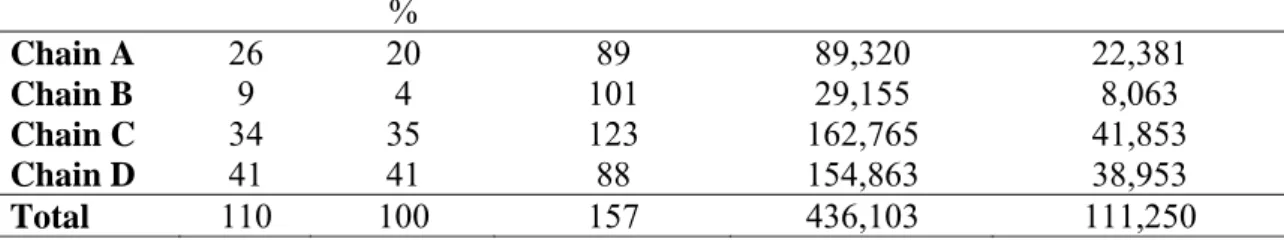
Table 1. Descriptive statistics No. stores Market share No. coffee items sold in each chain No. Weekly observations No. monthly observations % Chain A 26 20 89 89,320 22,381 Chain B 9 4 101 29,155 8,063 Chain C 34 35 123 162,765 41,853 Chain D 41 41 88 154,863 38,953 Total 110 100 157 436,103 111,250

(27)

Table 2. Coffee expenditure market share for each chain (%)

Chain A Chain B Chain C Chain D

Month 1 0.187 0.044 0.327 0.408 Month 2 0.190 0.042 0.342 0.395 Month 3 0.191 0.038 0.343 0.396 Month 4 0.187 0.034 0.332 0.418 Month 5 0.206 0.037 0.338 0.391 Month 6 0.212 0.034 0.323 0.403 Month 7 0.209 0.036 0.326 0.399 Month 8 0.186 0.034 0.339 0.413 Month 9 0.201 0.041 0.332 0.393 Month 10 0.179 0.041 0.347 0.375 Month 11 0.194 0.034 0.315 0.401 Month 12 0.174 0.043 0.323 0.400 Month 13 0.183 0.043 0.334 0.374 Month 14 0.220 0.039 0.321 0.363 Month 15 0.172 0.041 0.320 0.398 Min 0.172 0.034 0.315 0.363 Max 0.220 0.044 0.347 0.418

(28)

Table 3. Results for Price differences across chains: Aggregation over stores within a chain

Chain A Chain B Chain C Chain D

Chain A --- 0.0307 2.49 (0.115) 0.0374 3.76 (0.053) 0.0323 2.48 (0.115) Chain B --- 0.0067 0.14 (0.711) 0.0017 (0.01 (0.931) Chain C --- -0.0050 0.06 (0.8005) Chain D ---

*Indicates significance at the 5% level

Table 4. Results for Price differences across chains: No aggregation over stores within a chain

Chain A Chain B Chain C Chain D

Chain A --- 0.0313* 28.08 (<0.01) 0.0343* 78.88 (<0.01) 0.0326* 68.72 (<0.01) Chain B --- 0.0030 0.3 (0.585) 0.0013 0.05 (0.821) Chain C --- -0.0017 0.25 (0.6154) Chain D

(29)

Table 5. Index number estimates using different types of aggregation Months Month 1-2 Month 2-3 Month 3-4 Month 4-5 Month 5-6 Month 6-7 Month 7-8 Month 8-9

Laspeyres Homogeneity over chains 0.991 1.033 1.044 1.008 1.018 1.047 1.027 1.006

Homogeneity based on hedonics 0.994 1.037 1.049 1.018 1.034 1.059 1.036 1.011

No homogeneity over chains 1.001 1.042 1.058 1.024 1.040 1.064 1.040 1.018

No homogeneity over stores 1.003 1.044 1.059 1.026 1.043 1.070 1.040 1.019

Paasche Homogeneity over chains 0.982 1.016 1.023 0.983 1.005 1.037 1.016 0.993

Homogeneity based on hedonics 0.982 1.015 1.022 0.975 0.989 1.025 1.002 0.986

Fisher Homogeneity over chains 0.987 1.025 1.034 0.995 1.012 1.042 1.022 1.000

Homogeneity based on hedonics 0.988 1.026 1.035 0.996 1.011 1.042 1.019 0.999

Törnqvist Homogeneity over chains 0.987 1.025 1.034 0.995 1.012 1.042 1.022 1.000

Homogeneity based on hedonics 0.988 1.026 1.035 0.997 1.011 1.042 1.019 0.999

(30)

Table 5. Index number estimates using different types of aggregation (continued) Months Month 9-10 Month 10-11 Month 11-12 Month 12-13 Month 13-14 Month 14-15 Total % change

Laspeyres Homogeneity over chains 1.012 0.987 1.030 1.002 0.979 1.056 1.263 126.30 Homogeneity based on hedonics 1.017 0.991 1.037 1.005 0.983 1.060 1.380 138.04

No Homogeneity over chains 1.019 0.998 1.042 1.007 1.003 1.071 1.518 151.77

No homogeneity over stores 1.028 0.999 1.043 1.008 1.004 1.073 1.564 156.41

Paasche Homogeneity over chains 1.001 0.978 1.013 0.996 0.938 1.006 0.985 98.48 Homogeneity based on hedonics 0.998 0.973 1.009 0.991 0.932 1.003 0.903 90.26

Fisher Homogeneity over chains 1.007 0.982 1.021 0.999 0.958 1.031 1.115 111.52 Homogeneity based on hedonics 1.008 0.982 1.023 0.998 0.957 1.031 1.116 111.62

Törnqvist Homogeneity over chains 1.007 0.982 1.021 0.999 0.960 1.029 1.115 111.53 Homogeneity based on hedonics (NC) 1.007 0.982 1.023 0.998 0.960 1.029 1.118 111.78

(31)

Table 6. Monthly and total chained estimates of price change for each supermarket chain Month 1-2 Month 2-3 Month 3-4 Month 4-5 Month 5-6 Month 6-7 Month 7-8 Month 8-9 Laspeyres Chain A 1.011 1.043 1.056 1.005 1.088 1.044 1.103 0.988 Chain B 1.025 1.079 1.055 0.996 1.042 1.072 1.012 1.006 Chain C 0.983 1.052 1.065 1.020 1.026 1.053 1.017 1.013 Chain D 1.008 1.028 1.052 1.038 1.027 1.082 1.027 1.037 Paasche Chain A 0.996 0.994 1.030 0.936 0.956 0.971 1.044 0.964 Chain B 0.946 1.041 1.022 0.967 1.005 1.025 0.999 0.966 Chain C 0.952 1.034 1.023 0.975 1.013 1.025 0.991 0.998 Chain D 0.985 0.995 0.994 0.981 0.974 1.033 0.986 0.981 Fisher Chain A 1.003 1.018 1.043 0.970 1.020 1.007 1.073 0.976 Chain B 0.985 1.060 1.039 0.982 1.023 1.048 1.005 0.986 Chain C 0.967 1.043 1.044 0.997 1.020 1.039 1.004 1.005 Chain D 0.997 1.012 1.023 1.009 1.000 1.057 1.006 1.009 Törnqvist Chain A 1.003 1.018 1.043 0.972 1.021 1.006 1.073 0.976 Chain B 0.987 1.060 1.038 0.982 1.024 1.048 1.005 0.987 Chain C 0.968 1.043 1.044 0.997 1.020 1.039 1.004 1.005 Chain D 0.997 1.012 1.022 1.009 1.001 1.057 1.006 1.009

(32)

Table 6. Monthly and total chained estimates of price change for each supermarket chain (continued) Month 9-10 Month 10-11 Month 11-12 Month 12-13 Month 13-14 Month 14-15 Chained Total Laspeyres Chain A 1.057 0.987 1.067 0.992 0.992 1.171 177.86 Chain B 1.026 1.014 1.002 1.009 0.997 1.012 140.42 Chain C 0.986 1.021 1.024 0.999 0.995 1.020 130.60 Chain D 1.026 0.981 1.048 1.019 1.016 1.063 155.89 Paasche Chain A 1.021 0.944 1.015 0.966 0.847 1.032 73.63 Chain B 1.002 1.009 0.985 0.984 0.986 0.994 92.83 Chain C 0.978 1.007 1.003 0.979 0.967 1.002 94.62 Chain D 0.985 0.948 1.000 1.001 0.933 0.935 75.77 Fisher Chain A 1.039 0.965 1.041 0.979 0.917 1.099 114.44 Chain B 1.014 1.011 0.993 0.996 0.992 1.003 114.17 Chain C 0.982 1.014 1.014 0.989 0.981 1.011 111.16 Chain D 1.005 0.965 1.024 1.010 0.974 0.997 108.69 Törnqvist Chain A 1.038 0.965 1.040 0.979 0.924 1.094 114.87 Chain B 1.014 1.011 0.994 0.996 0.992 1.003 114.62 Chain C 0.982 1.014 1.014 0.989 0.981 1.011 111.26 Chain D 1.005 0.965 1.024 1.010 0.977 0.994 108.77

(33)

Appendix A

Akaike’s (1973) Information Criteria (AIC) and Schwartz’s (1978) Bayesian Information Criterion (BIC) can be written as follows (Kennedy, 1998):

AIC = T K T SSE 2 ln ⎟+ ⎠ ⎞ ⎜ ⎝ ⎛ _and BIC = ⎟ ⎠ ⎞ ⎜ ⎝ ⎛ + ⎟ ⎠ ⎞ ⎜ ⎝ ⎛ T T K T SSE ln ln ,

where T denotes the sample size, K is the number of regressors and SSE is the sum of squared errors.

The index number formulae used are as follows:

0 1 0 0 i it n i i t

p

w

Laspeyres

∑

=

1 0 1 0 − =

⎥

⎦

⎤

⎢

⎣

⎡

⎟⎟

⎠

⎞

⎜⎜

⎝

⎛

=

∑

it i n i it t

p

w

Paasche

( )⎟ ⎠ ⎞ ⎜ ⎝ ⎛ ₊

∏

⎥

⎦

⎤

⎢

⎣

⎡

⎟⎟

⎠

⎞

⎜⎜

⎝

⎛

=

it i w w i it t

p

rnqvist

o

T

0 2 1 0 0

&&

where pit is the price of item i in period t, for t = 0,…, T, and wi0 is good i’s share of total

expenditure in period 0.

The Fisher index is the geometric mean of the Laspeyres and Paasche indexes. For more on these indexes, see Diewert (1976).

The chained index number formula is:

t t t

P

₀

=

₀1

×

₁2

×

...

×

₋₁ , where P = any price index.

(34)

Appendix B

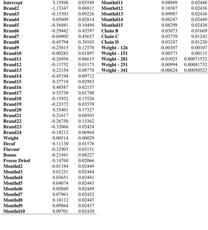
Table B1. Model 1 Results: Base Chain = Chain A Variable Parameter Estimate Standard Error Variable Parameter Estimate Standard Error Intercept 5.15948 0.03549 Monthd11 0.08809 0.02448 Brand2 -1.13347 0.06811 Monthd12 0.10387 0.02436 Brand3 -0.15303 0.09226 Monthd13 0.09987 0.02436 Brand4 0.05609 0.02814 Monthd14 0.08247 0.02449 Brand5 -0.56881 0.10494 Monthd15 0.08298 0.02430 Brand6 -0.29442 0.43597 Chain B 0.03073 0.01669 Brand7 -0.04905 0.45637 Chain C 0.03739 0.01243 Brand8 -0.45794 0.39103 Chain D 0.03247 0.01230 Brand9 -0.25815 0.12570 Weight - 126 -0.00307 0.00107 Brand10 -0.00283 0.01897 Weight - 151 0.00573 0.00115 Brand11 -0.26956 0.06615 Weight - 201 -0.01025 0.00071532 Brand12 -0.13752 0.03173 Weight - 251 0.00994 0.00081732 Brand13 0.23154 0.08778 Weight - 341 -0.00624 0.00050523 Brand14 -0.45194 0.09712 Brand15 0.37718 0.02983 Brand16 0.40587 0.02157 Brand17 0.52730 0.01780 Brand18 -0.15932 0.15526 Brand19 -0.23572 0.03570 Brand20 0.35401 0.17327 Brand21 0.21617 0.04503 Brand22 -0.26750 0.15362 Brand23 -0.32066 0.02424 Brand24 -0.18212 0.06964 Weight 0.00514 0.00029 Decaf 0.11130 0.01576 Flavour -0.32903 0.03151 Bonus -0.21941 0.08227 Freeze Dried 0.14760 0.02066 Monthd2 -0.01184 0.02449 Monthd3 0.01231 0.02444 Monthd4 0.03651 0.02441 Monthd5 0.04074 0.02443 Monthd6 0.05049 0.02449 Monthd7 0.07961 0.02432 Monthd8 0.10112 0.02445 Monthd9 0.09864 0.02437 Monthd10 0.09701 0.02430

(35)

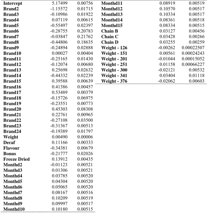
Table B2. Model 2 Results: Base Chain = Chain A Variable Parameter Estimate Standard Error Variable Parameter Estimate Standard Error Intercept 5.17499 0.00756 Monthd11 0.08919 0.00519 Brand2 -1.15572 0.01715 Monthd12 0.10570 0.00517 Brand3 -0.10986 0.01922 Monthd13 0.10334 0.00517 Brand4 0.07119 0.00615 Monthd14 0.08361 0.00518 Brand5 -0.55497 0.02397 Monthd15 0.08334 0.00515 Brand6 -0.28755 0.20783 Chain B 0.03127 0.00456 Brand7 -0.03847 0.21762 Chain C 0.03428 0.00266 Brand8 -0.44806 0.18635 Chain D 0.03255 0.00259 Brand9 -0.24894 0.02888 Weight - 126 -0.00262 0.00022507 Brand10 0.00027 0.00404 Weight - 151 0.00561 0.00024243 Brand11 -0.25165 0.01430 Weight - 201 -0.01044 0.00015052 Brand12 -0.12074 0.00680 Weight - 251 0.01158 0.00066227 Brand13 0.25698 0.02632 Weight - 300 -0.02121 0.00532 Brand14 -0.44332 0.02239 Weight - 341 0.03404 0.01118 Brand15 0.39588 0.00639 Weight - 376 -0.02062 0.00603 Brand16 0.41386 0.00457 Brand17 0.53489 0.00379 Brand18 -0.15726 0.06975 Brand19 -0.23551 0.00773 Brand20 0.45303 0.08308 Brand21 0.22761 0.00965 Brand22 -0.27108 0.03500 Brand23 -0.31367 0.00513 Brand24 -0.19389 0.01797 Weight 0.00490 0.00006 Decaf 0.11166 0.00333 Flavour -0.34381 0.00679 Bonus -0.21777 0.02026 Freeze Dried 0.13912 0.00435 Monthd2 -0.01123 0.00521 Monthd3 0.01306 0.00521 Monthd4 0.03785 0.00520 Monthd5 0.04304 0.00520 Monthd6 0.05065 0.00520 Monthd7 0.08167 0.00516 Monthd8 0.10209 0.00519 Monthd9 0.09997 0.00517 Monthd10 0.10180 0.00515