University of Cardiff
Urban
Morphology
and
Housing
Market
Athesissubmittedinpartialfulfillmentforthedegreeof DoctorofPhilosophy(PhD)
Yang
Xiao
B.ScinUrbanPlanning ȋʹͲͲȌ
M.ArchinUrbanDesign ȋʹͲͲͺȌ
APPENDIX 1:
Specimen layout for Thesis Summary and Declaration/Statements page to be included in a Thesis
DECLARATION
This work has not previously been accepted in substance for any degree and is not concurrently submitted in candidature for any degree.
Signed ……… (candidate) Date ………
STATEMENT 1
This thesis is being submitted in partial fulfillment of the requirements for the degree of ………(insert MCh, MD, MPhil, PhD etc, as appropriate)
Signed ……… (candidate) Date ………
STATEMENT 2
This thesis is the result of my own independent work/investigation, except where otherwise stated. Other sources are acknowledged by explicit references.
Signed ……… (candidate) Date ………
STATEMENT 3
I hereby give consent for my thesis, if accepted, to be available for photocopying and for inter-library loan, and for the title and summary to be made available to outside organisations. Signed ……… (candidate) Date ………
STATEMENT 4: PREVIOUSLY APPROVED BAR ON ACCESS
I hereby give consent for my thesis, if accepted, to be available for photocopying and for inter-library loans after expiry of a bar on access previously approved by the Graduate Development Committee.
Abstract
Urban morphology has been a longstanding field of interest for geographers but without adequate focus on its economic significance. From an economic perspective, urban morphology appears to be a fundamental determinant of house prices since morphology influences accessibility. This PhD thesis investigates the question of how the housing market values urban morphology. Specifically, it investigates people’s revealed preferences for street patterns. The research looks at two distinct types of housing market, one in the UK and the other in China, exploring both static and dynamic relationships between urban morphology and house price. A network analysis method known as space syntax is employed to quantify urban morphology features by computing systemic spatial accessibility indices from a model of a city’s street network. Three research questions are empirically tested. Firstly, does urban configuration influence property value, measured at either individual or aggregate (census output area) level, using the Cardiff housing market as a case study? The second empirical study investigates whether urban configurational features can be used to better delineate housing submarkets. Cardiff is again used as the case study. Thirdly, the research aims to find out how continuous change to the urban street network influences house price volatility at a micro-level. Data from Nanjing, China, is used to investigate this dynamic relationship. The results show that urban morphology does, in fact, have a statistically significant impact on housing price in these two distinctly different housing markets. I find that urban network morphology features can have both positive and negative impacts on housing price. By measuring different types of connectivity in a street network it is possible to identify which parts of the network are likely to have negative accessibility premiums (locations likely to be congested) and which parts are likely to have positive premiums (locations highly connected to destination opportunities). In the China case study, I find that this relationship holds dynamically as well as statically, showing evidence that price change is correlated with some aspects of network change.
I would like to dedicate this thesis to my wife and son,
who give me unconditional love, sacrifice, encouragement and propulsion for
Acknowledgements
I have spent almost three years to complete this research, in fact, during these time I am not fighting the war of PhD independently. This work would not have been completed without the great support and sincere help from many people.
First of all, I would like to thank my supervisors Prof. Chris Webster and Dr. Scott Orford for developing my knowledge of urban economics, and commenting and correcting successive drafts of the thesis in every detail, as well as their support, invaluable advice, patient guidance, encouragement and thoughtfulness through the completion of this study,
I would also like to thank Prof. Fulong Wu, Prof. Eric Heikkila, Alain Chiaradia, Dr. Yiming Wang, Dr. Fangzhu Zhang, Prof. Zhigang Li, and Prof. Xiaodong Song, for their insightful comments and advice, as well as their encouragement. I am grateful to all of the faculty and staff in the Cardiff school of planning and geography for their help.
I owe many thanks to my doctoral colleagues, especially Chris Zheng Wang, Chinmoy Sarkar, Agata Krause, Amanda Scarfi, Kin Wing Chan, II Hyung Park,
Tianyang GeˈDr. Jie Shen and Dr. Yi Li, for their help on improving my research.
Many thanks should be given to Chris Zheng Wang’s family, Xiaoyu Zhang, Chunquan Yu, Fan Ye, and Xin Yu, for offering their priceless friendship, hospitality, and practical help. I am grateful to all of my friends who are not physically around me but encourage me all the time.
Finally, I would like to thank my mother, my parents, parents-in-law, particularly my wife Mrs. Lu Liu and my son Sean Yaru Liu, for their supplication, support, sacrifice and encouragement throughout my life.
Contents
Chapter One: ... 1 Introduction ... 1 1.1 Background ... 1 1.2 Research questions ... 8 1.3 Thesis structures ... 11 Chapter Two: ... 14Hedonic housing price theory review ... 14
2.1 Introduction ... 14
2.2 Hedonic model: ... 15
2.2.1 Theoretical basis ... 16
2.2.2 Hedonic price criticism ... 21
2.2.3 Estimation criticism ... 23 2.3 Housing attributes ... 35 2.3.1 Structure characteristics ... 39 2.3.2 Locational characteristics ... 41 2.3.3 Neighborhood ... 47 2.3.4 Environmental ... 50 2.3.5 Others ... 53 2.4 Conclusion ... 54 Chapter Three: ... 58
Space syntax methodology review ... 58
3.1 Introduction ... 58
3.2 Overview of urban morphology analysis ... 59
3.3 Accessibility types ... 60
3.4 Space syntax algorithm ... 62
3.5 Critics of the space syntax method ... 68
3.6Developments of space syntax theory ... 73
3.6.1 Unique axial line map ... 74
3.6.2 Segment Metric Radius measurement ... 76
3.6.3 Angular segmentmeasurement ... 77
3.7 How urban morphology interacts with social economics phenomenon ... 78
3.8 Conclusion ... 83
Chapter Four: ... 87
Urban configuration and housing price... 87
4.1 Introduction ... 87
4.2 Locational information in hedonic models ... 89
4.3 Methodology ... 92
4.3.1 Space syntax spatial accessibility index ... 93
4.3.2 Hedonic regression model ... 94
4.4 Data and study area ... 95
4.4.1 Datasets ... 95
4.4.2 Study area... 97
4.5 Empirical results ... 102
4.5.3 Aggregate data ... 111
4.5.4 Discussion of disaggregated data and aggregated data ... 119
4.6 Conclusion ... 120
Chapter Five: ... 122
Identification of housing submarkets by urban configurational features ... 122
5.1 Introduction ... 122
5.2 Literature review ... 125
5.2.1Specifications of housing submarket ... 125
5.2.2 Accessibility and social neighborhood characteristics ... 130
5.3 Methodologies... 133
5.3.1 Space syntax... 133
5.3.2 Hedonic price model ... 133
5.3.3 Two-Step cluster analysis ... 134
5.3.4 Chow test ... 136
5.3.5 Weighted standard error estimation ... 137
5.4 Study area and dataset ... 137
5.5 Empirical analysis ... 138
5.5.1 Market-wide hedonic model ... 138
5.5.2 Specifications and estimations for submarkets ... 142
5.5.3 Estimation of weighed standard error ... 160
5.6 Conclusions ... 162
Identifying the micro-dynamic effects of urban street configuration on house price
volatility using a panel model ... 165
6.1 Introduction ... 165
6.2 Literature review ... 168
6.2.1 Cross-sectional static house price models ... 168
6.2.2 Hybrid repeat sales model with hedonic model ... 169
6.2.3 Panel models ... 171
6.3 Methodology ... 175
6.3.1 Space syntax method: ... 175
6.3.2 Panel model ... 175
6.4 Data and study area ... 178
6.4.1 Study area... 178
6.4.2 Data sources ... 183
6.5 Analysis and empirical results ... 192
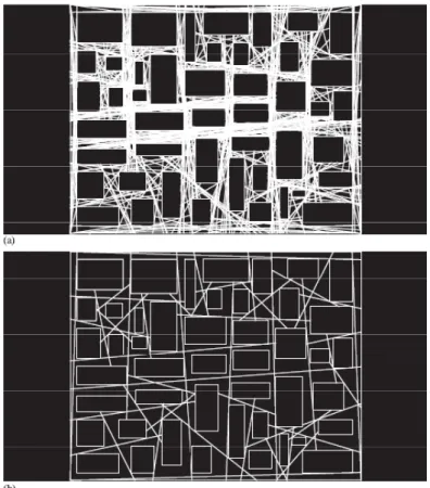
6.5.1 Street network analysis ... 192
6.5.2 Empirical results ... 195 6.6 Discussion ... 205 6.7 Conclusion ... 207 Chapter Seven: ... 209 Conclusions ... 209 7.1 Introduction ... 209
7.2 Conclusions for each chapter ... 209
7.3 Implications... 215
7.3.3 Implications for urban planning ... 217
7.4 Limitation of these studies ... 218
7.4.1 Imperfections of data quality ... 218
7.4.2 Econometrics issues ... 219
7.4.3 Space syntax axial line and radii ... 220
7.5 Recommendation for future studies ... 220
Reference ... 222
|
List of Tables
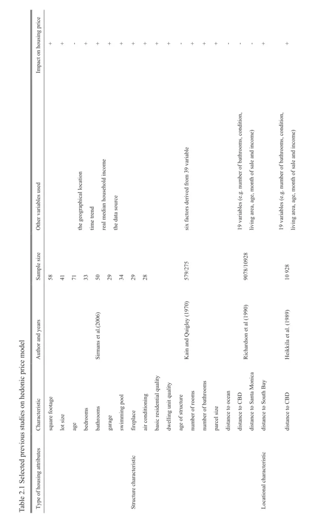
Table 2. 1 Selected previous studies on hedonic price model ... 37
Table 4. 1 The transaction number of each year ... 99
Table 4. 2 Fifty-five variables and Description ... 101
Table 4. 3 Descriptive Statistics for disaggregated dataset ... 103
Table 4. 4 Regression results of Model I (a) and (b) ... 107
Table 4. 5 White test for Model I (a) and (b) ... 108
Table 4. 6 Global Moran’s I for Model I (a) and (b) ... 108
Table 4. 7 Model I (c): Different Radii - T value comparisons ... 110
Table 4. 8 Descriptive Statistics for aggregated dataset... 111
Table 4. 9 Regression results of Model II (a) and (b) ... 115
Table 4. 10 White test for Model II (a) and (b) ... 116
Table 4. 11 Global Moran’s I for Model II (a) and (b) ... 116
Table 4. 12 Model II (c): Different Radii - T value comparisons ... 118
Table 4. 13 Comparison the results with previous studies ... 120
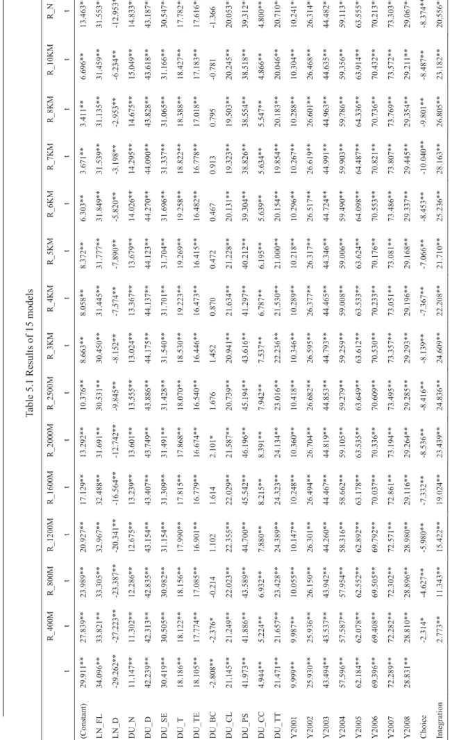
Table 5. 1 Results of 15 models ... 141
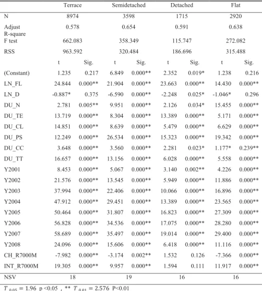
Table 5. 2 Estimation results of dwelling type specification ... 143
Table 5. 3 Chow test results of dwelling type specification ... 144
Table 5. 4 Estimation results of spatial nested specification ... 147
Table 5. 5 Chow test results of spatial nested specification ... 148
Table 5. 6 Cluster results of optimal urban configurational features specification ... 149
Table 5. 7 Descriptive of four submarkets ... 152
Table 5. 8 Estimation results of optimal urban configuration specification ... 154
Table 5. 9 Chow test results of optimal urban configuration specification... 154
Table 5. 10 Cluster results of nested urban configuration and building type specification ... 156
Table 5. 11 Descriptive of five submarkets ... 158
Table 5. 13 Chow test results of nested all urban configurational features and
building type specification ... 160
Table 5. 14 Estimation results of weighed standard error ... 161
Table 6. 1 General information of Nanjing from 2005-2010 ... 182
Table 6. 2 The changes of accessibility at different radii from 2005 to 2010 .... 186
Table 6. 3 The changes of mean of housing price from 2005 to 2010 ... 187
Table 6. 4 Statistics descriptive data ... 189
Table 6. 5 Empirical results of five models ... 195
Table 6. 6 F test for individual effects ... 199
Table 6. 7 Hausman Test ... 201
Table 6. 8 F test for individual effects and time-fixed effect ... 203
List of Figures
Figure 1. 1 Rent price pattern in Seattle ... 5
Figure 2. 1 Demand and offer curves of hedonic price function ... 18
Figure 2. 2 The marginal implicit price of an attribute as a function of supply and demand ... 20
Figure 2. 3 Accessibility measurement types ... 45
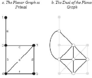
Figure 3. 1 Conventional graph-theoretic representation of the street network .. 62
Figure 3. 2 The process of converting the "Convex Space " to axial line map .... 64
Figure 3. 3 calculation of depth value of each street ... 65
Figure 3. 4 Integration map of London ... 67
Figure 3. 5 Value changes when deform the configuration ... 71
Figure 3. 6 Inconsistency of axial line ... 72
Figure 3. 7 Cross error for two axial line maps ... 73
Figure 3. 8 An algorithmic definition of the axial map ... 74
Figure 3. 9 Definition of axial line by AxialGen ... 75
Figure 3. 10 Notion of angular cost ... 77
Figure 4. 1 Study area of Cardiff, UK ... 98
Figure 4. 2 The Std. Dev. of housing price in output area units ... 100
Figure 4. 4 Locational characteristics t value change for model I (c) ... 111
Figure 4. 5 Locational characteristics t value change for model II (c) ... 118
Figure 5. 1 The t value change of all the variables via 15 models ... 142
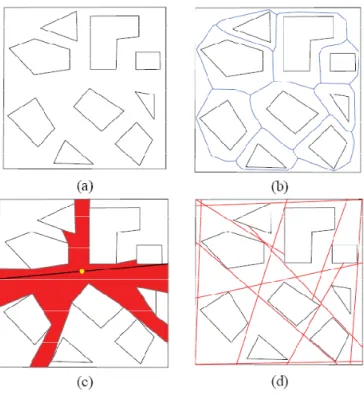
Figure 5. 2 Two-step cluster result of urban configuration feactures at 7km .... 149
Figure 5. 3 Two-step cluster result of nested dwelling type and all urban configurational features ... 157
Figure 6. 1 Location of Nanjing in China ... 181
Figure 6. 2 Study area of Nanjing ... 182
Figure 6. 5 Choice value change from 2005-2010 at different radii ... 194
Figure 7. 1 Diagrammatic structural equation of housing price ... 214
Figure A4. 1Integration at radii of 0.4 km ... 246
Figure A4. 2 Integration at radii of 0.8 km ... 246
Figure A4. 3 Integration at radii of 1.2 km ... 246
Figure A4. 4 Integration at radii of 1.6 km ... 246
Figure A4. 5 Choice at radii of 0.4 km ... 246
Figure A4. 6 Choice at radii of 0.8 km ... 246
Figure A4. 7 Choice at radii of 1.2 km ... 246
Figure A4. 8 Choice at radii of 1.6 km ... 246
Figure A4. 9 Integration at radii of 2 km ... 247
Figure A4. 10 Integration at radii of 2.5 km ... 247
Figure A4. 11 Integration at radii of 3 km ... 247
Figure A4. 12 Integration at radii of 4 km ... 247
Figure A4. 13 Choice at radii of 2 km ... 247
Figure A4. 14 Choice at radii of 2.5 km ... 247
Figure A4. 15 Choice at radii of 3 km ... 247
Figure A4. 16 Choice at radii of 4 km ... 247
Figure A4. 17 Integration at radii of 5 km ... 248
Figure A4. 18 Integration at radii of 6 km ... 248
Figure A4. 19 Integration at radii of 7 km ... 248
Figure A4. 20 Integration at radii of 8 km ... 248
Figure A4. 21 Choice at radii of 5 km ... 248
Figure A4. 22 Choice at radii of 6 km ... 248
Figure A4. 23 Choice at radii of 7 km ... 248
Figure A4. 24 Choice at radii of 8 km ... 248
Figure A4. 25 Integration at radii of 10 km ... 249
Figure A4. 27 Choice at radii of 10 km ... 249
Figure A4. 28 Global choice ... 249
Figure A6. 1 Integration at 0.8 km in 2005 ... 250
Figure A6. 2 Integration at .8 km in 2006 ... 250
Figure A6. 3 Integration at 0.8 km in 2007 ... 250
Figure A6. 4 Integration at 0.8 km in 2008 ... 250
Figure A6. 5 Integration at 0.8 km in 2009 ... 250
Figure A6. 6 Integration at 0.8 km in 2010 ... 250
Figure A6. 7 Choice at 0.8 km in 2005 ... 251
Figure A6. 8 Choice at 0.8 km in 2006 ... 251
Figure A6. 9 Choice at 0.8 km in 2007 ... 251
Figure A6. 10 Choice at 0.8 km in 2008 ... 251
Figure A6. 11 Choice at 0.8 km in 2009 ... 251
Figure A6. 12 Choice at 0.8 km in 2010 ... 251
Figure A6. 13 Integration at 1.2 km in 2005 ... 252
Figure A6. 14 Integration at 1.2 km in 2006 ... 252
Figure A6. 15 Integration at 1.2 km in 2007 ... 252
Figure A6. 16 Integration at 1.2 km in 2008 ... 252
Figure A6. 17 Integration at 1.2 km in 2009 ... 252
Figure A6. 18 Integration at 1.2 km in 2010 ... 252
Figure A6. 19 Choice at 1.2 km in 2005 ... 253
Figure A6. 20 Choice at 1.2 km in 2006 ... 253
Figure A6. 21 Choice at 1.2 km in 2007 ... 253
Figure A6. 22 Choice at 1.2 km in 2008 ... 253
Figure A6. 23 Choice at 1.2 km in 2009 ... 253
Figure A6. 24 Choice at 1.2 km in 2010 ... 253
Figure A6. 25 Integration at 2 km in 2005 ... 254
Figure A6. 26 Integration at 2 km in 2006 ... 254
Figure A6. 29 Integration at 2 km in 2009 ... 254
Figure A6. 30 Integration at 2 km in 2010 ... 254
Figure A6. 31 Choice at 2 km in 2005 ... 255
Figure A6. 32 Choice at 2 km in 2006 ... 255
Figure A6. 33 Choice at 2 km in 2007 ... 255
Figure A6. 34 Choice at 2 km in 2008 ... 255
Figure A6. 35 Choice at 2 km in 2009 ... 255
Figure A6. 36 Choice at 2 km in 2010 ... 255
Figure A6. 37 Integration at 5 km in 2005 ... 256
Figure A6. 38 Integration at 5 km in 2006 ... 256
Figure A6. 39 Integration at 5 km in 2007 ... 256
Figure A6. 40 Integration at 5 km in 2008 ... 256
Figure A6. 41 Integration at 5 km in 2009 ... 256
Figure A6. 42 Integration at 5 km in 2010 ... 256
Figure A6. 43 Choice at 5 km in 2005 ... 257
Figure A6. 44 Choice at 5 km in 2006 ... 257
Figure A6. 45 Choice at 5 km in 2007 ... 257
Figure A6. 46 Choice at 5 km in 2008 ... 257
Figure A6. 47 Choice at 5 km in 2009 ... 257
Figure A6. 48 Choice at 5 km in 2010 ... 257
Figure A6. 49 Integration at 8 km in 2005 ... 258
Figure A6. 50 Integration at 6 km in 2006 ... 258
Figure A6. 51 Integration at 8 km in 2007 ... 258
Figure A6. 52 Integration at 8 km in 2008 ... 258
Figure A6. 53 Integration at 8 km in 2009 ... 258
Figure A6. 54 Integration at 8 km in 2010 ... 258
Figure A6. 55 Choice at 8 km in 2005 ... 259
Figure A6. 57 Choice at 8 km in 2007 ... 259
Figure A6. 58 Choice at 8 km in 2008 ... 259
Figure A6. 59 Choice at 8 km in 2009 ... 259
Figure A6. 60 Choice at 8 km in 2010 ... 259
Figure A6. 61 Integration at 10 km in 2005 ... 260
Figure A6. 62 Integration at 10 km in 2006 ... 260
Figure A6. 63 Integration at 10 km in 2007 ... 260
Figure A6. 64 Integration at 10 km in 2008 ... 260
Figure A6. 65 Integration at 10 km in 2009 ... 260
Figure A6. 66 Integration at 10 km in 2010 ... 260
Figure A6. 67 Choice at 10 km in 2005 ... 261
Figure A6. 68 Choice at 10 km in 2006 ... 261
Figure A6. 69 Choice at 10 km in 2007 ... 261
Figure A6. 70 Choice at 10 km in 2008 ... 261
Figure A6. 71 Choice at 10 km in 2009 ... 261
Figure A6. 72 Choice at 10 km in 2010 ... 261
Figure A6. 73 Integration at 12 km in 2005 ... 262
Figure A6. 74 Integration at 12 km in 2006 ... 262
Figure A6. 75 Integration at 12 km in 2007 ... 262
Figure A6. 76 Integration at 12 km in 2008 ... 262
Figure A6. 77 Integration at 12 km in 2009 ... 262
Figure A6. 78 Integration at 12 km in 2010 ... 262
Figure A6. 79 Choice at 12 km in 2005 ... 263
Figure A6. 80 Choice at 12 km in 2006 ... 263
Figure A6. 81 Choice at 12 km in 2007 ... 263
Figure A6. 82 Choice at 12 km in 2008 ... 263
Figure A6. 83 Choice at 12 km in 2009 ... 263
Figure A6. 84 Choice at 12 km in 2010 ... 263
Figure A6. 87 Integration at 15 km in 2007 ... 264
Figure A6. 88 Integration at 15 km in 2008 ... 264
Figure A6. 89 Integration at 15 km in 2009 ... 264
Figure A6. 90 Integration at 15 km in 2010 ... 264
Figure A6. 91 Choice at 15 km in 2005 ... 265
Figure A6. 92 Choice at 15 km in 2006 ... 265
Figure A6. 93 Choice at 15 km in 2007 ... 265
Figure A6. 94 Choice at 15 km in 2008 ... 265
Figure A6. 95 Choice at 15 km in 2009 ... 265
Figure A6. 96 Choice at 15 km in 2010 ... 265
Figure A6. 97 Integration at 20 km in 2005 ... 266
Figure A6. 98 Integration at 20 km in 2006 ... 266
Figure A6. 99 Integration at 20 km in 2007 ... 266
Figure A6. 100 Integration at 20 km in 2008 ... 266
Figure A6. 101 Integration at 20 km in 2009 ... 266
Figure A6. 102 Integration at 20 km in 2010 ... 266
Figure A6. 103 Choice at 20 km in 2005 ... 267
Figure A6. 104 Choice at 20 km in 2006 ... 267
Figure A6. 105 Choice at 20 km in 2007 ... 267
Figure A6. 106 Choice at 20 km in 2008 ... 267
Figure A6. 107 Choice at 20 km in 2009 ... 267
Figure A6. 108 Choice at 20km in 2010 ... 267
Figure A6. 109 Global integration in 2005 ... 268
Figure A6. 110 Global integration in 2006 ... 268
Figure A6. 111 Global integration in 2007 ... 268
Figure A6. 112 Global integration in 2008 ... 268
Figure A6. 113 Global integration in 2009 ... 268
Figure A6. 115 Global choice in 2005 ... 269
Figure A6. 116 Global choice in 2006 ... 269
Figure A6. 117 Global choice in 2007 ... 269
Figure A6. 118 Global choice in 2008 ... 269
Figure A6. 119 Global choice in 2009 ... 269
1
Chapter One:
Introduction
``We shape our buildings, and afterwards our buildings shape us.’’ ---Winston Churchill
1.1
Background
Over the years, numerous conceptual, theoretical and empirical studies have attempted to formulate, model and quantify how the built environment is valued by people. However, studies of the valuation of urban morphology are rare, due to the lack of a powerful methodology to quantify the urban form accurately. In addition, neo-classical economic theories have emphasized location in respect to the city centre as the major spatial determinant of land value; but this has become weaker or even insignificant according to the findings of some current studies of mega cities, such as Los Angeles (Heikkila et al. 1989). Urban street networks contain spatial information on the arrangement of spaces, land use, building density, and patterns of movement and therefore give each location (or street segment) in the city a value in terms of accessibility. Thus, people can be thought of as paying for certain characteristics of the accessibility of the location of their choice. Moreover, they are likely to pay different amounts of money according to different demand levels.
The main motivation in this thesis is to investigate how urban morphology is valued. This is done through estimating its impact on the urban housing market, using the method of hedonic pricing. More specifically, the aim of this thesis is to examine whether street layout as an element of the urban form can provide extra spatial information in explaining the variance of housing price in a city, using both static and dynamic models.
Chapter 1
2
It is well known that commodity goods are heterogeneous, but that the unit of certain attributes or characteristics of the commodity good is treated as homogeneous (Lancaster 1966). Thus, people buy and consume residential properties as a bundle of “housing characteristics”, such as location, neighborhood and environmental characteristics. Hedonic analysis studies the marginal price people willing to pay for characteristics of that product. Rosen (1974b) pointed out that in theory in an equilibrium market, the implicit price estimated by a hedonic model is equal to the price per unit of a characteristic of the housing property that people are willing to pay. There are many studies that have followed Rosen’s approach in order to identify and value the characteristics that have an impact on housing price, including structural, locational, neighborhood and environmental characteristics (see for instance Sheppard, 1999;Orford, 2000; 2002).
Hedonic price models are widely used for property appraisal and property tax assessment purposes, as well as to construct house price indices. Furthermore, hedonic price models can be used for explanatory purposes (e.g. to identify the housing price premium associated with a particular neighborhood or design feature); and for policy evaluation or simulation purposes (e.g. to explore how the location of a new transit train might affect the property value; or whether the price premium associated with a remodeled kitchen will exceed the remodeling cost).
Orford (2002) notes that many hedonic studies are built upon the monocentric model of Alonso (1964) and Evans(1985), which underlined the importance of CBD as the major influence of land value and in which a bid-rent curve is translated into a negative house price curve (distance decay). Furthermore, in the early urban housing literature, the property value is differentiated based on its location and different sized units of homegenous housing units in a single market (Goodman and Thibodeau 1998). Thus, locational attributes (as the major determinant of land value) were the most important measure of hedonic housing price models. However, the monocentric
3
model has inherent limitations and has increasingly been criticized by researchers as both an overly simplistic modeling abstraction and an empirically historical phenomenon (e.g. Boarnet, 1994). The monocentric model excludes non-transportation factors, for instance in cases where persons do not choose their residential location based on the wish to minimize their commuting costs to their work place. Moreover, when metropolitan areas are in a state of restructuring, and suburban employment centers exist, numerous studies have shown that the impact of distance to CBD becomes weaker, unstable or even insignificant (Heikkila et al. 1989; Richardson et al. 1990; Adair et al. 2000). Cheshire and Sheppard (1997) also argued that much of the data used in hedonic analyses still lack land and location information. Moreover, hedonic modeling studies ignore the potentially rich source of information in a city’s road grid pattern. In order to understand people’s preferences for different locations, urban morphology seems to have the potential of a theoretical and methodological breakthrough, since it has the ability to capture numerically and mathematically both the form and the process of human settlements.
With regards to the study of urban morphology, frequently referred to as urban form, urban landscape and townscape, it grows and shapes in the later of the nineteenth century, and is characterized by a number of different perspectives, such as those taken by geography and architecture (Sima and Zhang 2009). The studies of urban form in Britain have been heavily influenced by M.R.G. Conzen. The Conzenian approach is more interested in the description, classification and exemplification of the characteristics of present townscapes based on survey results; an approach that could be termed as an “indigenous British geographical tradition ”. Later, this tended to shift from metrological analyses of plots to a wider plan-analysis (Sheppard 1974; Slater 1981).Recently the urban morphologists have come to examine the individuals, organizations and the process involved in shaping a particular element of urban form (Larkham 2006). In contrast, European traditions (e.g. Muratori1959,1963) take an architectural approach, stressing that elements, structures of elements, organism of
Chapter 1
4
structures are the components of urban form, which can also be called ‘procedural typology’(Moudon 1997).
However, studies of urban morphology from the perspective of both geographers and urban economist are mainly interested in how and why individual households and businesses prefer certain locations, and how those individual decisions add up to a consistent spatial pattern of land uses, personal and business transaction, and travel behavior. For example, Hurd (1903) first highlighted land-value is not homogenous on topography on the street layout. He argued that one of advantage of irregular street layout is to protect central growth rather than axial growth, which allows people quick access to or from the business center. A rectangular street layout permits free movement throughout a city, and the effect will be promoted by the addition of long diagonal streets. In his study, Washington as a political city in US. provides an typical example of diagonal streets, where the large proportion of space are taken up by streets and squares, while it is not a mode for a business city. Another contribution Hurd made is mapping the price per frontage foot of a ground plan for several cities in US., showing the scale of average value (width and depth), see the example of Seattle showed in figure (1.1). Although he explained that the ground rent is a premium paid solely for location and all rent is based on the location’s utility, the questions that why the high rental price located along linear as a axis, why there is bigger differentness of rental price despite how the streets approach to each other in the same area, and how to control the scale effects are not addressed.
Sour Web issu ͳǤͳ rce: Hurd (190 bster (2010) ues that Hur
03) ) takes an e rd did not a economist’s address. Stre 5 s approach a eet layout a
and has poi as the most inted out se essential el everal impor lement of u rtant urban
Chapter 1
6
form provides a basic geometry for accessibility, determining how street segments arrange possibilities and patterns of movement and transactional opportunities through ‘spatial configuration’. The network gives each location (or street segment) in the city a particular connectivity value, and each part of the city, each road, each plot of land and each building has its own value as a point of access to other places, people and organizations. The general (connectivity to everywhere else) value of any point in the grid is also a profoundly significant economic value signifying access to opportunities for cooperative acts of exchange between one specialist skill and all others within the urban economy. Put another way, the street grid shapes the cost of transactions between an urban labour force: it spatially allocates the economy’s division of labour. Thus, the geometric accessibility created by an urban grid is the most fundamental of all urban public goods. This being so, if it could be priced, it may be possible to allocate accessibility more efficiently. Measuring network-derived accessibility is the first step in so doing. It also allows for greater efficiencies in the design and planning of cities by governments and private developers when they build new infrastructure.
In spite of the crucial role of urban morphology to the urban economy, morphological studies are not a part of the mainstream planning literature, it seems, because verbal descriptions of properties cannot easily be translated into geometric abstractions and theories. In other words, it is lack of a sound scientific methodology for quantifying the urban form coherently. Early attempts were limited by the availability of software and hardware that could operate standard statistical approaches such as cluster analysis in order to research aspects of urban form (Openshaw 1973). The problems of establishing standard definitions in urban morphology and the perception that much of the information on urban form is not readily converted into ‘data’ has hindered the large-scale use of computers in storing and processing information. Alexander (1964, 1965) first introduced formal mathematical concepts into the debate in 1964.
7
A range of early works in formal urban morphology explored how mathematical formalism such as graph theory and set theory could work in the urban design arena (e.g. March and Steadman 1971, Martin and March 1972, Steadman 1983). By the end of twentieth century, one innovative system of theories and techniques had emerged; known as ‘Space Syntax’. It is an approach to urban form quite different from the British geographical tradition.
Space syntax originated as a quantified approach for spatial representation, which id developed in the 1970s at University College London. It is as a scientific and systematic way to study the interaction of people’s movement and building environment. In book of ‘The Social Logic of Space’, Hillier and Hanson (1984b) noted that the exploration of spatial layout or structure has great impact on human social activities. Recently, the approach has been refined by Hillier (1996), Penn (2003), and Hillier and Penn (2004), with particular focus on the arrangement of spaces and possibilities and patterns of movement through ‘spatial configuration’. Over the past two decades, space syntax theory has provided computational support for the development of urban morphological studies, revealing the characteristics of spaces in terms of movement and potential use. Space syntax has attempted to define the elements of urban form by measuring geometric accessibility; measuring the relationships between street segments by a series of measurements, such as connectivity, control, closeness and betweenness (Jiang and Claramunt 2002).
This thesis extends this tradition by employing space syntax methodology to refine hedonic price modeling. By so doing, it attempts to make a significant contribution to urban scholarship by exploring how finely measured urban morphology is associated with a number of housing market issues. In particular, I conduct a number of statistical experiments to find out how much people are willing to pay for different urban morphological attributes; or put another way, for different kinds of accessibility
Chapter 1
8
1.2
Research
questions
This dissertation addresses three research questions relevant with urban morphology and housing markets.
The first question has three aspects: (a) whether the accessibility information contained in an urban configuration network model has a positive or negative impact on housing price; (b) assuming such relationships exist, whether the network model determinants of urban morphology are stronger or weaker than traditional locational attributes (such as the distance to CBD); (c) whether the relationship is constant in both disaggregated and aggregated levels.
The monocentric urban economic model and polycentric variants emphasize location, hypothesizing that house prices decrease with a growing distance to the CBD, but more recent studies show that distance to CBD has become less important or even insignificant, suggesting either that people no longer choose their residential location based on minimum travel cost to work or that work has significantly dispersed within cities. Non-transportation factors (e.g. the distance to amenity and school quality), have become more influential in residential locations (White 1988a; Small and Song 1992).Therefore, many scholars attempt to explore the variety of preferences for location (e.g. the distance to a bus stop and distance to a park). However, these studies
need a priori specification within a pre-defined area, identifying local attractions
significant enough to influence locational choice systematically and measuring the proximity of the property to these attractive places.
However, this could cause econometric bias in the estimation, such as multicollinearity, spatial autocorrelation and omitting variables. The notion of general, systemic accessibility has been proven to better capture location options than the purely Euclidean distance in many studies on property value (e.g. Hoch and Waddell,
9
1993), as it indicates the ability of individuals to travel more generally and to participate in various kinds of activities at different locations (Des Rosiers et al. 2000). However, accessibility indicators measuring attractiveness or proximity to an opportunity are normally applied to studies at an aggregated level (e.g. Srour et al., 2002), and disaggregated level accessibility measures still tend to rely on Euclidean distance or time cost from a location to particular facilities.
The accessibility information contained in an urban street layout model would seem, in principle, a suitable approach for measuring locational characteristics at a disaggregated level without a pre-defined map of or knowledge about attractiveness hot spots. This dissertation explores this proposition and thus contributes to this important theoretical and methodological gap in the hedonic house-price modeling literature.
The second question deals with the identification of housing submarkets by urban configurational features; and comparing this approach with traditional specifications of housing submarkets, asks whether network-based specifications produce efficient estimation results. It is known that housing submarkets are important, and people's demand for particular attributes vary across space. But within submarkets, the price of housing (per unit of service) is assumed to be constant. Generally, there are two mainstream schools of thoughts for identifying submarkets: spatial specification and non-spatial specification. Spatial specification stresses a pre-defined geographic area within which people’s choice preferences are assumed to be homogeneous. This is criticized for being arbitrary. In contrast, non-spatial specification methods emphasize accuracy of estimation, advocating a data driven approach, which is criticized for being unstable over time (e.g. Bourassa et al.1999). These specifications for housing submarket are widely accepted in academic and practitioner fields in most developed countries with mature urban land markets. There is less knowledge about how to delineate sub markets in property markets of developing countries, where the building
Chapter 1
10
type in many fast growing cities is dominantly simplex (apartments) and social neighborhood characteristics are not long established and change quickly over time. This is the case in most cities in China.
This question contributes to another important gap in existing knowledge, as urban configuration features are assumed to be associated with both spatial information and people’s preference. A network-based method could provide a new alternative specification for housing submarket delimitation that extends the non-spatial method by adding more emphasis on people’s choice of location indirectly. The method could also help urban planners and government officials understand how different social economic classes respond to the accessibility of each location.
The third question has three aspects: (a) exploring micro-dynamic effects of urban configuration on housing price volatility; (b) asking whether this relationship is dynamic and synchronous over both space and time and whether submarkets exist as a result of this dynamic relationship; and (c)asking what kind street network improvements produce positive and negative spillover effects captured in property values.
The literature shows that most empirical analyses of house price movement focus on exploring the macro determinants of price movements over time using aggregate data, such as GDP, inflation indices and mortgage rates. Although some scholars state that accessibility could be a potential geographical determinant of house price volatility at a regional or city scale, there is little evidence confirming this relationship statistically. One reason for that is inaccurate measurements of accessibility(Iacono and Levinson 2011). In particular, it has proven difficult to measure changes inaccessibility at the disaggregated level, which is more reliant on Euclidean distance measures of accessibility. The premise of the research presented in this thesis, particularly in the chapter on China, hypothesizes that the continuous changes in urban street network
11
that are associated with urban growth and the attendant changes in accessibility, are partial determinants of micro-level house price volatility. This question is particularly relevant in China, where the profound institutional reforms of urban housing systems and breathtaking urban expansion, have meant numerous investments into road network developments aimed at the urban fringe in order to facilitate the rapid expansion of cities. The city of Nanjing, used as a case study in Chapter Six is a good example, providing an opportunity to empirically examine the dynamic relationship between housing price and urban configurational change.
The findings of this dissertation should be of great value to urban planners and government officials in addressing the problem of managing urban growth efficiently, understand the multi-scale positive and negative externalities of road networks as captured in housing markets, assisting property value assessment for tax purposes, and evaluating urban land use policies and planning regulations.
1.3
Thesis
structures
This thesis is organized into seven chapters.
After the introduction, chapter two investigates the literature on house price evaluation using the Hedonic price model. The approach covers several aspects, including the fundamental theory, theoretical criticisms, issues of estimation bias, and choice of housing attributes. In particular, the chapter focuses on the specification of the hedonic house price function form, housing submarkets and the debates on locational characteristics.
Chapter three provides a literature review of the methodology of space syntax-style network analysis. The basic notion of the space syntax method and the algorithms of
Chapter 1
12
Then, some key criticisms of space syntax are summarised. Finally, the chapter reviews empirical evidence on how urban morphology interacts with socio-economic phenomenon.
Chapters of four to six present theoretical and empirical analysis, which addresses the thesis’ three research questions, respectively. In order to clearly delineate the theoretical contribution of each question, separate specific literature reviews are provided in each chapter.
Using a semi-log hedonic price functional form, chapter four adopts a part of the metropolitan area of Cardiff, UK as a case study to examining whether urban configurational features can impact the property value at both individual and output area level.
Chapter five uses the same Cardiff dataset, examining whether urban configurational features can be considered as an efficient specification alternative for identifying housing submarkets, especially when there is no predefined spatial boundary. Two-step clustering analysis is discussed in chapter and the results of a network approach to housing market delineation are compared to the results of two traditional approaches.
Chapter six setup a panel study of multi-year house prices to examine whether the continuous changes in urban street network associated with urban growth and the attendant changes in accessibility are partial determinants of micro-level house price volatility. This chapter uses the case of Nanjing, China in the time period from 2005 to 2010.The Space syntax method is employed in this chapter to track changes in accessibility within the urban street layout over time.
13
the discussions of the three empirical chapters and presents brief reflections on the policy implications of the results. The chapter ends with comments on the limitations of the experiments presented in the thesis and with recommendations for future studies in this field.
Chapter 2
14
Chapter Two:
Hedonic housing price theory review
2.1
Introduction
The most commonly applied methods of housing price evaluation can be broadly divided into two groups: traditional and advanced methods. There are five traditional mainstream standard recognized valuation methods in the field of property valuation: comparative method (comparison), contractor’s method (cost method), residual method (development method), profits method (accounts method), investment method (capitalization/income method).Advanced methods include techniques such as hedonic price modeling, artificial neural networks (ANN), case-based reasoning and spatial analysis methods.
Hedonic price modeling is the most commonly applied of these. Many scholars (e.g. Griliches, 1961) have referred to the work of Court (1939) as an early pioneer in applying this technique. He used the term hedonic to analyze price and demand for the individual sources of pleasure, which could be considered as attributes combined to form heterogeneous commodities. It was an important early application of multivariate statistical techniques to economics.
In this chapter, several aspects of hedonic modeling will be investigated in-depth, including the theoretical basis, the theoretical criticism, estimation criticism, and its use in pricing housing attributes, including accessibility (the subject of this thesis). Accordingly, the conclusion will mainly focus on the theoretical aspects of hedonic price modeling that are relevant to the question of which function form to choose in this study.
15
2.2
Hedonic
model:
In regards to the theoretical foundations, the hedonic model is based on Lancaster’s (1966) theory of consumer’s demand. He recognized a composite good whose units are homogeneous, such that the utilities are not based on the goods themselves but instead the individual “characteristics” of a good – its composite attributes. Thus, the consumers make their purchasing decision based on the number of characteristics a good as well as per unit cost of each characteristic. For example, when people choose a car, they would consider the quantity of characteristics from a car, such as fast acceleration, enhanced safety, attractive styling, increased prestige, and so on.
Although Lancaster was the first to discuss hedonic utility, he says nothing about pricing models. Rosen (1974a) was the first to present a theory of hedonic pricing. Rosen argue that an item can be valued by its characteristics, in that case, an item’s total price can be considered as sum of price of each homogeneous attributes, and each attribute has a unique implicit price in a equilibrium market. This implies that an item’s price can be regressed on the characteristics to determine the way in which each characteristic uniquely contributes to the overall composite unit price.
As Rothenberg et al. (1991) describes, the hedonic approach has two significant advantages over alternative methods of measuring quality and defining commodities in housing markets. First, compressing the many characteristics of housing into one dimension allows the use of a homogenous commodity assumption; and thus, the hedonic construction avoids the complications and intractability of multi-commodity models. Furthermore, the hedonic approach reflects the marginal tradeoffs that both supplier and demanders make among characteristics in the markets, so that differences in amounts of particular components will be given the weights implicitly prevailing in the market place.
Chapter 2
16
2.2.1 Theoretical basis
Housing constitutes a product class differentiated by characteristics such as number of rooms and size of lot. Freeman III (1979b) argued that the housing value can be considered a function of its characteristics, such as structure, neighborhood, and
environmental characteristics. Therefore, the price function of house ݄݅ can be
demonstrated as
ܲ ൌ ܲሺܵଵǡ ǥ ǡ ܵǡ ǥ ǡ ܰଵǥ ǡ ܰǥ ǡ ܳଵǥ ǡ ܳሻ Equation (2.1)
Where:
Theܵ, ܰ and ܳ indicate the vectors of site, neighborhood, and environmental
characteristics respectively.
Empirical estimation of Equation (2.1) involves applying one of a number of statistical modeling techniques to explain the variation in sales price as a function of
property characteristics. Let X represent the full set of property characteristics (ܵ,
ܰand ܳ) included in the empirical model. The empirical representation of the ݅th
housing price is:
୧ ൌ ሺ୧ǡȕǡİሻ Equation (2.2)
Where
Ⱦis a vector of parameters to be estimate
ɂis a stochastic residual term
17
Such as hedonic price models aim at estimating implicit price for each attributes of a good, and a property could be considered as a bunch of attributes or services, which are mainly divided into structural, neighborhood, accessibility attributes and etc. Individual buyers and renters, for instance, try to maximize their expected utility, which are subject to various constraints, like their money and time.
Freeman (1979) explains that a household maximizes its utility by simultaneously moving along each marginal price schedule, where the marginal price of a household’s willingness to pay for an unit of each characteristic should equal to the marginal implicit price of that housing attribute. This clearly locates the technique within a neo-classical economics framework – a framework that analytically computes prices on the assumption that markets equilibrate under an ‘invisible hand’ with perfect information and no transaction costs. It is noted that although the theory of hedonics has been developed with this limiting theoretical context discussed above, the technique is typically applied as an econometric empirical model and does not rely on the utility maximization underlying theory.
To understand if a household is in equilibrium, the marginal implicit price associated with the chosen housing bundle is assumed equal to the corresponding marginal willingness to pay for those attributes. To unpack this, I begin with considering how a market for heterogeneous goods can be expected to function, and what type of equilibrium we can expect to observe.
Chapter 2
18
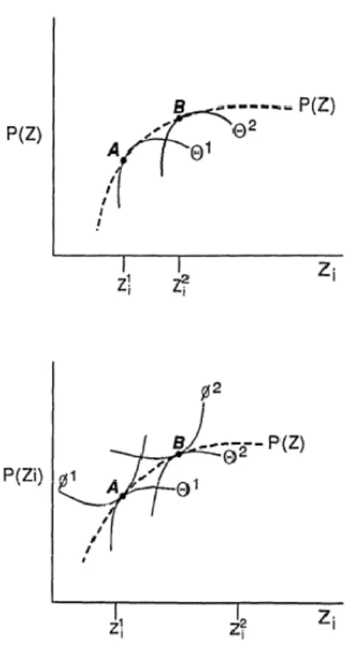
Figure 2.1 Demand and offer curves of hedonic price function Source: Follain and Jimenez, 1985; pp.79
Following Follain and Jimenez’s works (1985), a utility function can interpret a
household decision,ሺǡ ሻ, where x is a composite commodity whose price is unity,
and z is the vector of housing attributes. Assume that households want to maximize
utility subject but with the budget constraint ൌ ሺሻ , where y is the annual
household income. The partial derivative of the utility function with respect to a housing attribute is the household’s marginal willingness to pay function for that
attribute. A first order solution requires୳
୳౮ ൌ ୧ ൌ
ப୮ሺሻ
பሺሻ, i=1,…,n, under the usual
properties of u.
19
ߠሺݖǡ ݑǡ ݕǡ ܽሻ Equation (2.3)
Where ܽ is a parameter that differs from household to household.
This can be characterized as the trade-off a household is willing to make between alternative quantities of a particular attribute at a given income and utility level, whilst
remaining indifferent to the overall composition of consumption.
ݑ ൌ ݑሺݕ െ ߠǡ ݖǡ ܽሻ Equation (2.4)
ߠ1 pictured in the upper panel of fig.(2.2) show that when solving the schedule for ߠ.
ߠ1 represented by households is everywhere indifferent along ߠ1 and ߠ schedules
that are lower, which depend on its higher utility levels. It can be shown that
ߠ ൌ ௨
௨ೣ Equation (2.5)
which is the additional expenditure a consumer’s willingness to pay for another unit
of ݖand beequally well off (i.e. the demand curve). Figure 2.2 denotes two such
equilibria: a for householdߠ1 and
Chapter 2
20
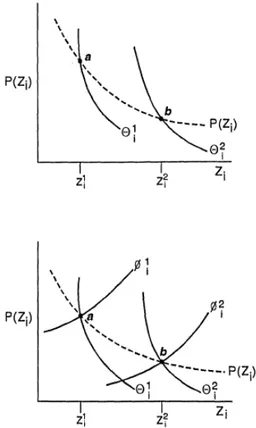
Figure 2.2 The marginal implicit price of an attribute as a function of supply and demand Source: Follain and Jimenez, 1985; pp.79
The supply side could also be considered, as p(z) is determined by the market,. When P (Z) as given, and constant returns to scale are assumed, each firm’s costs per unit
are assumed to be convex and can be denoted as ܿሺݖǡ ߚሻ, where the ߚ denotes factor
price and production-function parameters. The firm then maximizes profits per unit
ߨ ൌ ሺݖሻ െ ܿሺݖǡ ߚሻ, which would yield the condition that the additional cost of
providing that ݅th characteristics,ܥ , is equal to the revenue that can be gained, so
that ൌ ܿ .
Rosen (1974) emphasized that in fact the function ܲis determined by a market in a
clearing condition, where the amount of commodities offered by sellers at every point must equal to amounts demanded by consumers choosing. Both consumers and
21
producer base their locational and quantity decisions on maximizing behavior and equilibrium prices are determined so that buyers and sellers can be perfectly scheduler. Generally, a market-clearing price are determined by the distributions of consumer tastes as well as producer costs.
However, Rosen did not formally present a functional form for the hedonic price function, his model clearly implies a nonlinear pricing structure.
2.2.2 Hedonic price criticism
One of the most important assumptions to come under attack is the one relating to perfect equilibrium. For this assumption to hold, it requires perfect information and zero transaction costs (Maddison 2001). If the equilibrium condition does not hold,
the implicit prices derived from hedonic analysis are biased, because there is no a
priori reason to suppose that the extent of disequilibrium in any area is correlated with
the levels if particular amenities contributing to the hedonic house price. The consequence of disequilibrium is likely to be in increased variance in results rather systematic bias (Freeman III 1993). Furthermore, Bartik (1987) and Epple (1987) also point out that the hedonic estimation is not to the result of demand-supply interaction, as in the hedonic model, an individual consumer decision does not affect the hedonic price function, which implies that an individual consumer’s decision cannot affect the suppliers.
Follain and Jimenez (1985) argue that the marginal price derived from the hedonic function does not actually measure a particular household is willing to pay for a unit of a certain characteristic. Rather, it is a valuation that is the result of demand and supply interactions in the entire market. Under the restrictive condition of homogeneous preferences – another limitation of the neo-classical model - the hedonic equation can reveal the underlying demand parameters for the representative
Chapter 2
22
household. When all households are similar with homogenous characteristics of income and socio-economic and supplies are different, the hedonic coefficient will be the marginal willingness to pay. Only in extreme cases when all consumers have identical incomes and utility functions will the marginal implicit price curve be identical to the inverse demand function for an attribute. With identical incomes and utility functions, these points all fall on the same marginal willingness to pay curve (Freeman 1979). Hence, the implicit price of an attribute is not strictly equal to the marginal willingness to pay, and hence demand for that attribute.
Another issue raised by Freeman (1979) is the speed of adjustment of the market to changing condition of supply and demand. If adjustment is not complete, observed marginal implicit price will not accurately measure household marginal willingness to pay. When the demand for an attribute is increasing, marginal implicit prices will underestimate true marginal willingness to pay. This is because marginal willingness to pay will not be translated into market transactions that affect marginal implicit price until the potential utility gains pass the threshold of transactions and moving cost.
Finally, the market for housing can be viewed as a stock-flow model where the flow is a function form, but the price at any point in time is determined only by the stock at that point in time. This raises a concern about the accuracy of the price data itself. Given that the data is based on assessments, appraisals, or self-reporting, it may not correspond to actual market price. The errors in measuring the dependent variable will tend to obscure any underlying relationship between true property value measures and environment amenities. But the estimation of the relationship will not be biased unless the errors themselves are correlated with other variables in the model.
23
2.2.3 Estimation criticism
The hedonic price model relies on regression technology, which is criticized by some authors for a series of econometric problems that can lead to the bias of estimation, such as function specification, spatial heterogeneity, spatial autocorrelation, housing quality change, multicollinearity and heteroscedasticity.
2.2.3.1 Function specification
Hedonic models are sensitive to choice of functional form, as economic theory gives no clear guidelines on how to select the functional form. Rosen (1974a) demonstrated that the hedonic price functional form is a reduced form equation which reflect mechanisms of both supply and demand. A further important task facing researchers is how to function the relationships of dependent variable and the explanatory variables naturally, which impose an incorrect functional form on the regression equation will lead to misspecification bias. The simple approach is the ordinary linear approach, but if the true functional form of the hedonic equation is not linear, there will occur inconsistent estimation in the resulting coefficients (Linneman 1980). Freeman (1979) specified the Box-Cox transformation, which allows choice of the proper function form based on the structure of a particular data set. Typically, hedonic price regression models can be classified into four simple parametric functional forms;
a. Linear specification: both the dependent and explanatory variables enter the
regression with linear form.
ൌȕ σ ȕ୩୩
୩ୀଵ İ Equation (2.6)
Where:
p denotes the property value. İ is a vector of random error term
Chapter 2
24
characteristic ୩ of the good.
b. Semi-log specification: in a regression function, dependent variable is log form and
explanatory variable is linear , or dependent variable is linear and explanatory variable is log form.
ൌ Ⱦ σ Ⱦ୩୩
୩ୀଵ ɂEquation Equation (2.7)
Where:
p denotes the property value.
ɂis a vector of random error term
ȕ୩ (k = 1, . . . ,K) indicates the rate at which the price increases at a certain level,
given the characteristics x
c. Log-log specification: in a regression function, both the dependent and explanatory
variables are their log form.
ൌ ȕ σ ȕ୩୩
୩ୀଵ İEquation Equation (2.8)
Where:
p denotes the property value.
ɂis a vector of random error term
Ⱦ୩ (k = 1, . . . ,K) indicates how many percent the price p increases at a certain
level, if the kth characteristic xk changes by one percent.
d. Box-Cox transform: determine the specific transformation from the data itself then
enter the regression in individual transformed form.
ሺșሻ ൌȕ σ୩ୀଵȕ୩୩ሺȜౡሻİ Equation (2.9) Where: ሺሻ ൌ ሺሻെ ͳ Ʌ ǡ Ʌ ് Ͳ ൌ ǡ Ʌ ൌ Ͳ ሺౡሻ ൌ ሺౡሻെ ͳ ɉ୩ ǡ ɉ୩് Ͳ ൌ ୩ǡ ɉ୩ൌ Ͳ
25
From the Box-Cox transform equation we can see if the Ʌ and ɉ୩ are equal to 1, the
model will transform to the basic linear form. If the Ʌ and ɉ୩ are equal to 0, the
model will transform to the log-linear form. If the value Ʌ is equal to 0 and ɉ୩ are
equal to 1, then the model can be the semi-log form.
2.2.3.2 Debate about the hedonic function
Unfortunately, economic theory provides little guidance, and there is no specific function form for the hedonic price models suggested by Rosen (1974), Freeman (1979), Halverson and Pollakowski (1981) and Cassel and Mendelsohn (1985), so it is reasonable to try several functional forms to find the best performance. Among the four types of function forms in hedonic literatures, the semi-logarithmic form is much more prevalent, as it is easy to interpret its coefficients as the proportionate change in price arising from a unit change in the value of the characteristic. Furthermore, unlike log-log models, the semi-log model can deal with dummy variables for characteristics that are either present or absent (0 or 1). Diewert (2003) argued that the errors from a semi-log hedonic function are homoskedastic (have a constant variance).
Although more and more researchers prefer to use the Box-Cox transformation function, letting the dataset drive the function form, Cassel and Mendelsohn (1985) pointed out four inconsistencies of the Box-Cox transformation. Firstly, the large number of coefficients estimated with Box-Cox reduce the accuracy of any single coefficient, which could lead to poorer estimates of price. Secondly, the traditional Box-Cox functional form is not suited to any data set containing negative numbers. Furthermore, the Box-Cox function may be invalid for prediction, as the mean predicted value of the untransformed dependent variable need not equal the mean of the sample upon which is estimated. The predicted untransformed variables will be biased, and the predicted untransformed variables may also be imaginary. Fourth, the nonlinear transformation results in complex estimate of slopes and elasticities, which
Chapter 2
26
are often too cumbersome to use properly.
Taking least error as the choice criterion, Crooper et al. (1988) compared six function forms: linear, semi-log, double-log, Box-Cox linear, quadratic and quadratic Box-Cox, testing the best goodness of fit using data for Baltimore. His studies found that no function produced the lowest ȕi for all the attributes, although the quadratic Box-Cox function had the lowest normalized errors. However, the linear Box-Cox function had the lowest error variance, and based on the criterion, the linear Box-Cox performed the best and quadratic and double-log functions the worst. On the other hand, when variables are replaced or omitted, the Box-Cox linear function was the best of the six.
Having said all this, Halvorsen and Pollakowski (1981)rightfully pointed out that the true hedonic function form is unknown: we can only estimate it for any particular data set, although as I have shown, we do have methods to help choose the most appropriate parametric hedonic function form.
2.2.3.3 Housing submarkets
Housing property cannot be regarded as a homogeneous commodity. A unitary metropolitan housing market is unlikely ever to exist. Instead it is likely to be composed of interrelated submarkets (Adair et al. 1996; Tu 1997; Goodman and Thibodeau 1998; Whitehead 1999; Watkins 2001). Straszheim (1974) suggested that the housing market is a series of single markets, which requires different hedonic functions. According to Schnare and Stuyk (1976), housing submarkets arise when competition in a housing market is insufficient to ensure spatial equalization of physical housing attributes. Thus, the submarkets existence is the results of inelasticity (or high inelasticity) of demand and supply of housing at least in a short term. Bau and Thibodeau (1998) define housing sub-market as follows:
27
“Housing submarket are typically defined as geographic area where the prices per unit of housing quantity (defined using some index of housing characteristic) are constant.”(Bau and Thibodeau, 1998).
Goodman and Thibodeau (1998) argue that the existence of submarket questions the validity of the traditional assumption that urban housing markets can be modeled on the basis of a single market-wide house price equation. Adair et al. (1996), also argue that the failure to accommodate the existence of housing submarket will introduce bias and error into regression-based property valuation. Orford (2000), demonstrates that submarkets could be considered as relatively homogeneous sub-groups of the metropolitan housing market, people’s the preference on each housing attribute may vary in different submarkets whilst remain the same within each submarket. However, the theory assumes that the implicit price for per unit of each housing attribute is stationary over space, and this assumption ignores that different geographical demand and supply characterized by different classes of people can lead to the spatial disequilibrium of housing market in a metropolitan area. Thus, parameters estimated by a simple hedonic function for the whole market sometimes seems misleading.
Goodman and Thibodeau (2007) emphasize that housing submarkets are important in house price modeling for several reasons. Firstly, the assigning of properties to housing submarkets is likely to increase the accuracy of the prediction of the statistical models, which are used to estimate house prices. Secondly, identifying housing submarket boundaries within metropolitan areas will increase the chance of researchers deriving better spatial and temporal variations in their models of prices. Thirdly, the accurate allocation of properties to submarkets will improve the abilities of lenders and investors to price the risk related to the financing of homeownership. Finally, the provision of submarket boundary information to housing consumers will decrease their search costs.
Chapter 2
28
In terms of the specification of housing submarkets, Goodman and Thibodeau (1998) stated that a metropolitan housing market might be segmented into groups of submarkets according to the factor of demand and / or supply. Watkins (2001) also suggests that housing submarkets exist as dwelling can generate different price due to the interaction between segmented demand characterized by consumer groups, and segmented supply characterized by product groups. As such, housing submarkets may be defined by dwelling type (e.g., town house, flat and detached house); by structural characteristics (numbers of bedroom, and building style); by neighborhood characteristics (e.g., school quality). Alternatively, housing markets may be segmented by age, income and race of households (Schnare and Struyk 1976; Gabriel and Wolch 1984a; Munro 1986; Allen et al. 1995). In that case, higher income households tend to be willing to pay more for housing (per unit of housing services)and the attributes of other home-owners - to protect the homogeneity of their neighborhood, life chances of children and so on. Finally, racial discrimination may produce separate housing submarkets for majority and minority households (King and Mieszkowski 1973). Several empirical studies of submarkets have, found that spatial characteristics are more important than structure characteristics. Ball and Kirwan (1977) found housing affordability and the availability of mortgage finance to be important shapers of sub markets, despite spatial constraints. Historical characteristics can also contribute to housing market segmentation. More recently, scholars have been more aware of the importance of both spatial and structural factors as the specification criterions of housing submarket (Adair et al. 1996; Maclennan and Tu 1996).
Although, many researchers agree on a sub-market definition based on structural and locational features, there is little consensus as to how a submarket should be identified in practice. The most common procedure for testing submarket existence was introduced by Schnare and Struyk (1976) and has been employed subsequently (for example, Dale-Johnson 1982, Munro 1986). The test procedure involves three stages.
29
First, hedonic house price functions are estimated for each potential market segment in order to compare the submarket price for a `standard' dwelling. Secondly, a chow test is computed in order to show whether there are significant differences between the submarket specific prices. Thirdly, a weighted standard error is calculated for the submarket model, which acts as a further `common-sense' test of the significance of price differences for standard dwellings in different submarkets. This procedure also enables us to do a comparison of the effects on the accuracy of the house price models when different submarket definitions and stratification schemes are being compared.
Bourassa et al.(1999) stressed the need to test whether boundaries of submarkets are stable over time. Adding a dynamic part to the analysis makes it even more difficult to specify sub-market models since markets are constantly changing.
2.2.3.4 Spatial autocorrelation
A further discussion in terms of the application of hedonic price modeling is spatial dependency, also known as spatial autocorrelation. One of the basic assumptions underlying the regression model is that observations should be independent of one another. However, from the first law of geography, attributed to Tobler (1970), ‘everything is related to everything else, but near things are more related than distant things’, the independence of observations assumption is clearly a problem. Spatial
autocorrelation is concerned with the degree to which objects or activities at some place in the earth’s surface are similar to other objects or activities located nearby (Goodchild 1986). This is important in the sense that it is a special feature of spatial data (Can 1990); for example, houses that are close in geographic space are likely to have similar attributes. Generally, if the spatial effect is ignored, it is more likely that the real variance of the data is underestimated and thus leads to bias of the results (Ward and Gleditsch 2008). According to the works of Dunse et al. (1998), Bowen
Chapter 2
30
et al. (2001), Gillen et al. (2001), and Orford (1999), there are at least three sources of spatial autocorrelation, including property characteristics, the evaluation process; and mis-specification in the OLS model.
Firstly, spatial dependency exists because nearby properties, have similar property characteristics, in particular for structural features, as the properties were developed at the same time and also share the same locational conditions (Gillen et al. 2001; Bourassa et al. 2005).Secondly, spatial autocorrelation also arises from the valuation process, as the transaction price agreed between buyers and sellers will affect the price of the surrounding area (Bowen et al. 2001), especially where valuers use the comparison method, which is most common in the residential real estate industry. Thirdly, mis-specification of a model can result in spatial autocorrelation (Orford 1999), when the model is missing important variables, has extra unimportant variables, and / or an unsuitable functional form. Anselin (1988) also states that spatial autocorrelation is associated with spatial aggregation, the presence of uncontrolled-for non-li