Conditional Normalizing Flows for
Low-Dose Computed Tomography Image Reconstruction
Alexander Denker1 Maximilian Schmidt1 Johannes Leuschner1 Peter Maass1 Jens Behrmann1
Abstract
Image reconstruction from computed tomogra-phy (CT) measurement is a challenging statistical inverse problem since a high-dimensional condi-tional distribution needs to be estimated. Based on training data obtained from high-quality re-constructions, we aim to learn a conditional den-sity of images from noisy low-dose CT mea-surements. To tackle this problem, we propose a hybrid conditional normalizing flow, which integrates the physical model by using the fil-tered back-projection as conditioner. We eval-uate our approach on a low-dose CT bench-mark and demonstrate superior performance in terms of structural similarity of our flow-based method compared to other deep learning based approaches.
1. Introduction
Many important applications in medical imaging, such as computed tomography (CT) or magnetic resonance imag-ing (MRI), can be formulated as an inverse problem. The inverse problem consists in the reconstruction of an inter-nal image of a patient based on radiological data. Many of these applications are ill-posed inverse problems, as small measurement errors can result in large errors in the recon-struction. In a classical way, an inverse problem is often formulated as follows: A forward operatorA : X → Y maps the imagex†to (noisy) measurements
yδ=Ax†+µ, (1)
whereµdescribes the noise. The research in inverse prob-lems is focused in particular on developing algorithms for obtaining stable approximations of the true solutionx†. In
1
University of Bremen, Center for Industrial Mathemat-ics. Correspondence to: Alexander Denker < [email protected]>, Maximilian Schmidt < [email protected]>, Johannes Leuschner<[email protected]>. Second workshop on Invertible Neural Networks, Normalizing Flows, and Explicit Likelihood Models (ICML 2020), Virtual Conference
Figure 1.Ground truth samples from the LoDoPaB-CT dataset containing artifacts. These errors stem from the reconstruction technique that was used on the normal-dose measurements.
order to cover the uncertainties that occur especially with ill-posed problems, the theory of Bayesian inversion con-siders the posterior distributionp(x|yδ)(Dashti & Stuart,
2017). This posterior is the conditional density of the im-agexconditioned on the measurementsyδ.
The main task in statistical inverse problems is to ap-proximate this high-dimensional conditional distribution. For high-dimensional, structured images, like they arise in CT, this is a challenging process. In the field of density estimation, conditional normalizing flows (NF) (Winkler et al., 2019; Ardizzone et al., 2019b) allow to learn expres-sive conditional densities by maximum likelihood training. Since the physical model is known in CT (Eq. 2), we pro-pose a hybrid approach which integrates model-based re-construction with conditional NFs.
In many CT image reconstruction tasks the mean squared error (MSE) is used (Chen et al., 2017; He et al., 2020), which, however, has many known limitations (Zhao et al., 2017). In the context of maximum likelihood estimation (MLE), the MSE loss arises from the assumption of i.i.d. standard Gaussian noise. However, this assumption is vi-olated in CT training data since they are often obtained from reconstructions of high-dose or normal-dose measure-ments. E.g. the choice of the reconstruction algorithm can lead to artifacts, as shown in Figure 1. This implies that the reconstruction error for individual pixels is no longer inde-pendent. We argue that these dependencies can be better captured by a flow-based model.
Our contributions are twofold: 1) We apply conditional normalizing flows to CT image reconstruction. 2) We propose a hybrid approach, which integrates the physical model by using the filtered back-projection as conditioner. 1.1. Related Work
Deep learning methods have been successfully applied to many ill-posed inverse problems such as CT (Arridge et al., 2019). In particular, end-to-end learned meth-ods have been used. Those methmeth-ods can be classified in three main groups: post-processing (Chen et al., 2017), fully-learned (He et al., 2020) and learned iterative algo-rithms (Adler & ¨Oktem, 2018). These end-to-end methods have in common that they learn a parameterized operator Tθ:Y →Xby optimizing the parametersθusing training
data{(yδ i, x
†
i)}Ni=1. Usually, this is done by minimizing the MSE between the ground truth datax†i and the reconstruc-tionTθ(yδi)as ˆ θ∈arg min θ∈Θ 1 N N X i=1 kTθ(yδi)−x † ik 2.
Recently, Deep Image Priors were used for CT, achieving promising results in the low-data regime (Baguer et al., 2020). Similar to our approach is the work of (Adler &
¨
Oktem, 2018), who employed a Wasserstein GAN to draw samples from the conditional distribution. However, in this approach it is not possible to evaluate the likelihood of the generated samples. (Ardizzone et al., 2019a) have used invertible neural networks to approximate the con-ditional distribution and to analyze inverse problems. In a subsequent paper this concept was extended to condi-tional invertible neural networks (cINNs) which yielded good performance in the field of conditional image gen-eration (Ardizzone et al., 2019b).
2. Background on Computed Tomography
Computed tomography allows for a non-invasive acquisi-tion of the inside of the human body, which makes it one of the most important tools in modern medical imaging (Buzug, 2008). CT is a primary example of an inverse prob-lem. The determination of the interior distribution cannot be achieved directly. It has to be inferred from the mea-sured attenuation of X-rays sent through the body.Current research focuses on reconstruction methods for low-dose CT measurements to reduce the health risk from radiation (Shan et al., 2019; Baguer et al., 2020). One strat-egy to reduce the dose is to measure at fewer angles. This can result in undersampled measurements and therefore in the existence of ambiguous solutions to the inverse prob-lem. Another option is to lower the intensity of the X-ray. This leads to increased Poisson noise on the measurements
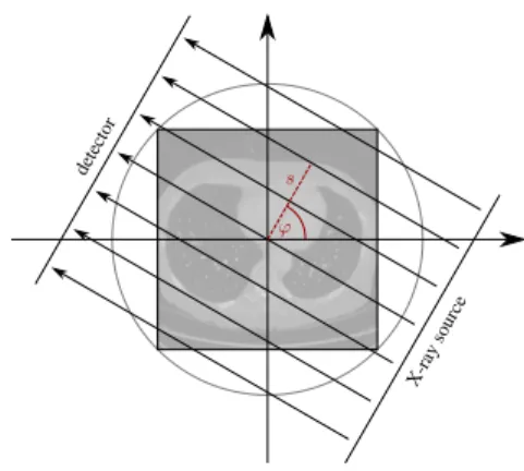
ϕ s
X-ray source detector
Figure 2.Schematic illustration of a CT scanner with a parallel beam geometry (Baguer et al., 2020). The scanner is rotated around the patient during the measurement.
and adds to the instability of the inversion. In this paper, we test our reconstruction model for the lower intensity case. The basic principle of a CT machine with a parallel beam geometry can be described by the 2D Radon transformA: X →Y (Radon, 1986): Ax(s, ϕ) = Z R x s cos(ϕ) sin(ϕ) +t −sin(ϕ) cos(ϕ) dt. (2)
It is an integration along a line, which is parameterized by the distances∈Rand angleϕ∈[0, π](cf. Figure 2). For
a fixed pair(s, ϕ)this results in the log ratio of initial and final intensity at the detector for a single X-ray beam (Beer-Lambert’s law). The whole measurement, calledsinogram, is the collection of the transforms for all pairs(s, ϕ). The task in CT is to invert this process to get a reconstruction of the body. The inversion of the Radon transform is an ill-posed problem since the operator is linear and compact (Natterer, 2001). The consequences is an instable inverse mapping, which amplifies even small measurement noise. A common inversion model is the filtered back-projection (FBP) (Shepp & Logan, 1974). The reconstruction for po-sition (i, j)is calculated by a convolution overs and an integration alongϕas
x(i, j) = Z π
0
y(s, ϕ)? h(s)|s=icos(ϕ)+jsin(ϕ)dϕ.
In general,his chosen as a high-pass filter such as the Ram-Lak filter (Ramachandran & Ram-Lakshminarayanan, 1971). In reality, we can only measure for a finite number of angles and distances. In this discrete setting the FBP only works well for a high number of measurement angles. Otherwise severe streak artifacts can appear in the reconstruction.
3. Methods
3.1. Problem SettingTo estimate conditional densities, data pairs from measure-mentsyδand ground truth imagesx†are required. In com-puted tomography (CT) it is not possible to obtain actual ground truth data, because no picture can be taken of the interior of the human body. Instead of using ground truth images we use reconstructions based on high-dose mea-surementsyδ1 = Ax†+µ
1, i.e. xδ1 = TFBP(yδ1). Be-causexδ1 is the output of an reconstruction algorithms, it can contain artifacts and differ from the actual image x†, see Figure 1 for an example. In the next step we sim-ulate low-dose CT measurements using this reconstruc-tion as yδ2 = Axδ1 +µ
2, where Var[µ2] ≥ Var[µ1], since low-dose measurements are more prone to measure-ment noise. The training set then consists of data pairs
{yδ2, xδ1}. An example of such a dataset is LoDoPaB-CT (Leuschner et al., 2019), which we use to benchmark our proposed conditional flow.
3.2. Normalizing Flow with FBP Conditioning
From a statistical point-of-view, an inverse problem can also be seen as a generating processx ∼ p(x|y)(Dashti & Stuart, 2017; Arridge et al., 2019). The task in such a statistical inverse problem is to estimate this conditional distribution. We are using conditional normalizing flows (NF) (Winkler et al., 2019) to approximate the target den-sityp(x|y). The conditional NF is composed of a series of invertible transformations F = fK ◦ · · · ◦f1. Here, every individual transformation is parameterized byθand receives a conditional inputy: fi = fθi(·, y). This
trans-formation defines a transport map, which converts the ini-tial density into a simple, easy-to-sample densitypZ. This
model defines a conditional densityq(x|y, θ)and using the change-of-variables formula the conditional density can be calculated: q(x|y;θ) =pZ(Fθ(x;y)) det ∂F θ(x;y) ∂x .
We denote the Jacobian for one data pointxi, yiwithJi = ∂Fθ(xi;yi)
∂x . Instead of directly using the measurementsyias
conditional inputs, we propose to employ a reconstruction, e.g. the filtered back-projectionxˆi=TFBP(y).
Assume a dataset{(xi, yi)}Ni=1of measurementsyiand
re-constructionsxi. To approximate the target densityp(x|y)
a conditional NFq(x|y, θ)can be trained using the negative log-likelihood as a loss function. Using a standard normal distribution, i.e.pZ∼ N(0, I), this amounts to minimizing
L(θ) = 1 N N X i=1 kFθ(xi;TFBP(yi))k22 2 −log|detJi|.
3.3. Conditional coupling layers
We are using the conditional coupling layer from (Ardiz-zone et al., 2019b) to construct a conditional invertible neu-ral network (cINN), which is an extension of the affine cou-pling layer from (Dinh et al., 2017). We propose to in-tegrate the model-driven approach of inverse problems by using the filtered back-projectionxˆ = TFBP(y)as condi-tional input instead of the raw sinogramm measurementsy. The inputu= [u1, u2]to an affine coupling layer is split into two parts and both parts are transformed individually:
v1=u1exp(s1(u2,x)) +ˆ t1(u2,x)ˆ v2=u2exp(s2(v1,x)) +ˆ t2(v1,x).ˆ
The transformationss1, s2, t1, t2do not need to be invert-ible and are modelled as convolutional neural networks (CNNs). The inverse of an affine coupling layer is:
u1= (v1−t1(u2,x))ˆ exp(−s1(u2,x))ˆ u2= (v2−t2(v1,x))ˆ exp(−s2(v1,x)).ˆ The log-determinant of the Jacobian for one affine cou-pling layer can be calculated as the sum over si, i.e. P
js1(u2,x)ˆ j+Pjs2(v1,x)ˆ j. A deep invertible network
can be built as a sequence of multiple such layers, with a permutation of the dimensions after each layer.
The conditional inputxˆis added as an extra input to each transformation in the coupling layer. In practice, an ad-ditional conditioning networkH is added, so instead ofxˆ the outputH(ˆx)is used. This conditioning networkH is under no architectural constraints and can contain all usual elements (i.e. BatchNorm, pooling layer, etc.) of a CNN.
4. Results
Sampling from the model is a two-step process: First, a samplezis drawn from the base densitypZ. Second, this
sample is transformed by the inverse to obtain an image. By repeatedly samplingzjfor a fixed inputyδwe thus estimate
the conditional mean as ˆ x=Ez[F−1(z, TFBP(yδ))]≈ 1 n n X j=1 F−1(zj, TFBP(yδ)).
We evaluate our model on the LoDoPaB-CT dataset (Leuschner et al., 2019). For this dataset we are in the case of oversampling, so we expect a uni-modal distribu-tion. This enables the choice of the conditional mean as the reconstruction method. If a highly multi-modal distribution is expected, the conditional mean is not the optimal choice. To measure the error between reconstruction and ground truth, the PSNR and the SSIM (Wang et al., 2004) are eval-uated. Both are common quality metrics for the evaluation of CT and MRI reconstructions (Joemai & Geleijns, 2017;
Groundtruth Filtered Backprojection
Conditioned Mean Conditioned Standard Deviation
Figure 3.Reconstruction and standard deviation of cINN. 1000
Samples were used for the reconstruction. The top row shows the ground truth image and the corresponding FBP.
Adler & ¨Oktem, 2018; Zbontar et al., 2018). The PSNR is a pixel-wise metric which is defined via the MSE. The SSIM is a structural metric, which compares local patterns of pixels and is not calculated on a per pixel basis.
4.1. Implementation
We follow the multi-scale architecture design of RealNVP (Dinh et al., 2017). After each block, consisting of 6 cou-pling layers, downsamcou-pling is performed. The downsam-pling is done using the Haar downsamdownsam-pling from (Ardiz-zone et al., 2019b) and the variant used in (Jacobsen et al., 2018). The dimensions have to be permuted after each cou-pling layer. This is done using the invertible 1x1 convo-lutions from (Kingma & Dhariwal, 2018). The model is implemented using the library FrEIA1. A conditioning net-work was used to further extract features from the filtered back-projection. This conditioning network was trained to-gether with the full flow-based model. Details on the im-plementation can be found in the supplementary material. 4.2. LoDoPaB-CT Dataset
We evaluate our method on the low-dose parallel beam (LoDoPaB) CT dataset (Leuschner et al., 2019), which con-tains over40 000 two-dimensional CT images and corre-sponding simulated low photon count measurements. The ground truth images xδ1 are human chest CT reconstruc-tions from the LIDC/IDRI database (Armato III et al., 2011), cropped to362×362pixels. Projections are com-puted using parallel beam geometry with1000angles and
1https://github.com/VLL-HD/FrEIA
513beams. Poisson noise is applied to model a low photon count (µ2in Section 3.1).
4.3. Evaluation on LoDoPaB-CT
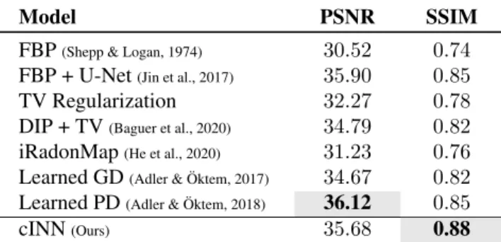
We have evaluated our model on the LoDoPaB-CT dataset. First we examined the dependence of PSNR and SSIM on the number of samples for the conditional mean. The re-sults are shown in Figure 4 (appendix). Both PSNR and SSIM increase with a higher number of samples. This al-lows for a trade-off between quality of reconstruction and time. For our evaluation we have chosen a conditional mean with 1000 samples. Table 1 shows the scores on the test dataset. The comparison includes several classical and deep learning approaches.
In terms of PSNR our model is comparable to other state-of-the-art deep learning approaches, despite not explicitly trained to minimize the MSE between the prediction and the ground truth images. Regarding the SSIM our model outperforms all other approaches. This further underlines our hypothesis that using the more flexible flow objective enable to incorporate structural properties.
Model PSNR SSIM
FBP(Shepp & Logan, 1974) 30.52 0.74 FBP + U-Net(Jin et al., 2017) 35.90 0.85
TV Regularization 32.27 0.78
DIP + TV(Baguer et al., 2020) 34.79 0.82 iRadonMap(He et al., 2020) 31.23 0.76 Learned GD(Adler & ¨Oktem, 2017) 34.67 0.82 Learned PD(Adler & ¨Oktem, 2018) 36.12 0.85
cINN(Ours) 35.68 0.88
Table 1.Results on the LoDoPaB-CT test set. The baseline meth-ods were evaluated in (Baguer et al., 2020).
5. Conclusion
We have investigated how flow-based models can be ap-plied as a conditional density estimator for the reconstruc-tion of low-dose CT images. Using this generative ap-proach, we were able to obtain high-quality reconstruc-tions that outperformed all other deep learning approaches in terms of structural similarity. So far only coupling-based INNs were used, but future work should explore other ar-chitectures such as i-ResNets (Behrmann et al., 2019) for this conditional density estimation task. Furthermore, our hybrid approach that integrates the physical model into the conditioning could enable the use of more advanced reconstruction algorithms. Thus, conditional flows are a promising avenue for statistical model-based inverse prob-lems such as CT reconstruction.
References
Adler, J. and ¨Oktem, O. Deep bayesian inversion. arXiv preprint, arXiv:1811.05910, 2018.
Adler, J. and ¨Oktem, O. Learned primal-dual reconstruc-tion. IEEE Transactions on Medical Imaging, 37(6): 1322–1332, 06 2018. doi: 10.1109/TMI.2018.2799231. Adler, J. and ¨Oktem, O. Solving ill-posed inverse prob-lems using iterative deep neural networks.Inverse Prob-lems, 33(12):124007, 11 2017. doi: 10.1088/1361-6420/aa9581.
Ardizzone, L., Kruse, J., Rother, C., and K¨othe, U. Ana-lyzing inverse problems with invertible neural networks. In7th International Conference on Learning Represen-tations, ICLR, 2019a.
Ardizzone, L., L¨uth, C., Kruse, J., Rother, C., and K¨othe, U. Guided image generation with conditional invert-ible neural networks. arXiv preprint, arXiv:1907.02392, 2019b.
Armato III, S. G., McLennan, G., Bidaut, L., McNitt-Gray, M. F., Meyer, C. R., Reeves, A. P., Zhao, B., Aberle, D. R., Henschke, C. I., Hoffman, E. A., Kazerooni, E. A., MacMahon, H., van Beek, E. J. R., Yankelevitz, D., Biancardi, A. M., Bland, P. H., Brown, M. S., Engel-mann, R. M., Laderach, G. E., Max, D., Pais, R. C., Qing, D. P.-Y., Roberts, R. Y., Smith, A. R., Starkey, A., Batra, P., Caligiuri, P., Farooqi, A., Gladish, G. W., Jude, C. M., Munden, R. F., Petkovska, I., Quint, L. E., Schwartz, L. H., Sundaram, B., Dodd, L. E., Fenimore, C., Gur, D., Petrick, N., Freymann, J., Kirby, J., Hughes, B., Vande Casteele, A., Gupte, S., Sallam, M., Heath, M. D., Kuhn, M. H., Dharaiya, E., Burns, R., Fryd, D. S., Salganicoff, M., Anand, V., Shreter, U., Vastagh, S., Croft, B. Y., and Clarke, L. P. The Lung Image Database Consortium (LIDC) and Image Database Resource Ini-tiative (IDRI): A completed reference database of lung nodules on CT scans. Med. Phys., 38(2):915–931, 02 2011. ISSN 0094-2405. doi: 10.1118/1.3528204. Arridge, S., Maass, P., ¨Oktem, O., and Sch¨onlieb,
C.-B. Solving inverse problems using data-driven models.
Acta Numerica, 28:1–174, 2019. ISSN 0962-4929. doi: 10.1017/S0962492919000059.
Baguer, D. O., Leuschner, J., and Schmidt, M. Com-puted tomography reconstruction using deep image prior and learned reconstruction methods. arXiv preprint, arXiv:2003.04989, 2020.
Behrmann, J., Grathwohl, W., Chen, R. T. Q., Duvenaud, D., and Jacobsen, J.-H. Invertible residual networks. InProceedings of the 36th International Conference on Machine Learning, volume 97, pp. 573–582, 2019.
Buzug, T. Computed Tomography: From Photon Statistics to Modern Cone-Beam CT. Springer Berlin Heidelberg, 2008. ISBN 9783540394082. doi: 10.1007/978-3-540-39408-2.
Chen, H., Zhang, Y., Kalra, M. K., Lin, F., Chen, Y., Liao, P., Zhou, J., and Wang, G. Low-dose CT with a residual encoder-decoder convolutional neural net-work. IEEE Transactions on Medical Imaging, 36 (12):2524–2535, 12 2017. ISSN 0278-0062. doi: 10.1109/TMI.2017.2715284.
Dashti, M. and Stuart, A. M. The Bayesian Approach to Inverse Problems, pp. 311–428. Springer International Publishing, Cham, 2017. ISBN 978-3-319-12385-1. doi: 10.1007/978-3-319-12385-1 7.
Dinh, L., Sohl-Dickstein, J., and Bengio, S. Density es-timation using real NVP. In 5th International Confer-ence on Learning Representations, ICLR 2017, Toulon, France, April 24-26, 2017, Conference Track Proceed-ings, 2017.
He, J., Wang, Y., and Ma, J. Radon inversion via deep learning. IEEE Transactions on Medical Imaging, 39 (6):2076–2087, 2020.
Jacobsen, J.-H., Smeulders, A., and Oyallon, E. i-RevNet: Deep invertible networks. ICLR 2018 - International Conference on Learning Representations, 2018. Jin, K. H., McCann, M. T., Froustey, E., and Unser, M.
Deep convolutional neural network for inverse problems in imaging. IEEE Transactions on Image Processing, 26(9):4509–4522, 09 2017. ISSN 1057-7149. doi: 10.1109/TIP.2017.2713099.
Joemai, R. M. S. and Geleijns, J. Assessment of structural similarity in CT using filtered backprojection and iter-ative reconstruction: a phantom study with 3D printed lung vessels. The British Journal of Radiology, 90 (1079):20160519, 2017. doi: 10.1259/bjr.20160519. PMID: 28830200.
Kingma, D. P. and Ba, J. Adam: A Method for Stochas-tic Optimization. arXiv preprint, arXiv:1412.6980, 12 2014.
Kingma, D. P. and Dhariwal, P. Glow: Generative flow with invertible 1x1 convolutions. In Bengio, S., Wallach, H. M., Larochelle, H., Grauman, K., Cesa-Bianchi, N., and Garnett, R. (eds.), Advances in Neural Information Processing Systems 31, pp. 10236–10245, 2018. Leuschner, J., Schmidt, M., Baguer, D. O., and Maaß, P.
The LoDoPaB-CT Dataset: A benchmark dataset for low-dose CT reconstruction methods. arXiv preprint, arXiv:1910.01113, 2019.
Natterer, F. The mathematics of computerized tomogra-phy. Classics in applied mathematics ; 32. Society for Industrial and Applied Mathematics, Philadelphia, 2001. ISBN 9780898714937. doi: 10.1137/1.9780898719284. Radon, J. On the determination of functions from their integral values along certain manifolds. IEEE Transac-tions on Medical Imaging, 5(4):170–176, 12 1986. ISSN 0278-0062. doi: 10.1109/TMI.1986.4307775.
Ramachandran, G. N. and Lakshminarayanan, A. V. Three-dimensional reconstruction from radiographs and elec-tron micrographs: Application of convolutions instead of fourier transforms. Proceedings of the National Academy of Sciences, 68(9):2236–2240, 1971. ISSN 0027-8424. doi: 10.1073/pnas.68.9.2236.
Shan, H., Padole, A., Homayounieh, F., Kruger, U., Khera, R. D., Nitiwarangkul, C., Kalra, M. K., and Wang, G. Competitive performance of a modularized deep neural network compared to commercial algorithms for low-dose CT image reconstruction. Nature Machine Intel-ligence, 1(6):269–276, 2019. ISSN 2522-5839. doi: 10.1038/s42256-019-0057-9.
Shepp, L. A. and Logan, B. F. The fourier reconstruction of a head section. IEEE Transactions on Nuclear Science, 21(3):21–43, 1974.
Wang, Z., Bovik, A. C., Sheikh, H. R., and Simoncelli, E. P. Image quality assessment: from error visibility to structural similarity. IEEE Transactions on Image Pro-cessing, 13(4):600–612, 04 2004. ISSN 1057-7149. doi: 10.1109/TIP.2003.819861.
Winkler, C., Worrall, D., Hoogeboom, E., and Welling, M. Learning likelihoods with conditional normalizing flows.arXiv preprint, arXiv:1912.00042, 2019.
Zbontar, J., Knoll, F., Sriram, A., Muckley, M. J., Bruno, M., Defazio, A., Parente, M., Geras, K. J., Katsnelson, J., Chandarana, H., Zhang, Z., Drozdzal, M., Romero, A., Rabbat, M., Vincent, P., Pinkerton, J., Wang, D., Yakubova, N., Owens, E., Zitnick, C. L., Recht, M. P., Sodickson, D. K., and Lui, Y. W. fastMRI: An open dataset and benchmarks for accelerated MRI. arXiv preprint, arXiv:1811.08839, 2018.
Zhao, H., Gallo, O., Frosio, I., and Kautz, J. Loss functions for image restoration with neural networks.IEEE Trans-actions on Computational Imaging, 3(1):47–57, 2017. doi: 10.1109/TCI.2016.2644865.
6. Appendix
6.1. Model Architecture
The model was trained for15.000stochastic gradient steps of batchsize10with the Adam-Optimizer (Kingma & Ba, 2014) using a weight decay of10−5. The last layer in the subnetworks of each coupling layer is initialized with zero. This initializes the model as a whole with the identity. A multiscale architecture was used for implementation of the cINN. The model includes 6 resolution levels. After each level a part of the channels is split off and passed on to the output. After each resolution level downsam-pling is performed. Downsamdownsam-pling was performed using the iRevNet variant (Jacobsen et al., 2018) as well as the Haar Downsampling by (Ardizzone et al., 2019b). The in-put size of the CT-images is1×352×352. The full cINN was build as follows.
cINN Output size
iRevNet-Downsampling 4×176×176 level 1 conditional section 4×176×176 iRevNet-Downsampling 16×88×88 Split:8×88×88to output 8×88×88 level 2 conditional section 8×88×88 iRevNet-Downsampling 32×44×44 Split:16×44×44to output 16×44×44 level 3 conditional section 16×44×44 iRevNet-Downsampling 64×22×22 Split:32×22×22to output 32×22×22 level 4 conditional section 32×22×22 Haar-Downsampling 128×11×11 Split:96×11×11to output 32×11×11 level 5 conditional section 32×11×11 Split:28×11×11to output 4×11×11 level 6 Dense-conditional section 484
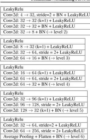
A conditioning network was used to extract features from the conditional input. Similar to the cINN, this network consists of 6 resolution levels. The output from the resolu-tion level of the condiresolu-tioning network is used as the condi-tioning input for the respective resolution level in the cINN. If not specified otherwise, a kernel size ofk= 3is used. In addition, batch normalization (BN) is applied.
Conv2d:1→3, stride=2 + LeakyReLU Conv2d:32→64+ LeakyReLU Conv2d:64→128+ BN + LeakyReLU Conv2d:128→64+ BN + LeakyReLU Conv2d:64→32+ BN + LeakyReLU Conv2d:32→4+ BN (→level1)
LeakyRelu
Conv2d:4→32, stride=2 + BN + LeakyReLU Conv2d:32→32(k=1) + LeakyReLU Conv2d:32→32+ BN + LeakyReLU Conv2d:32→8+ BN (→level2) LeakyRelu
Conv2d:8→32(k=1) + LeakyReLU Conv2d:32→64, stride = 2+ LeakyReLU Conv2d:64→16+ BN (→level3) LeakyRelu
Conv2d:16→64(k=1) + LeakyReLU Conv2d:64→64, stride = 2+ LeakyReLU Conv2d:64→32+ BN (→level4) LeakyRelu
Conv2d:32→96(k=1) + LeakyReLU Conv2d:96→128, stride = 2+ LeakyReLU Conv2d:128→32(k=1) + BN (→level5) LeakyRelu
Conv2d:32→64, stride=2 + LeakyReLU Conv2d:64→256, stride = 2+ LeakyReLU Average Pooling + Flatten + BN (→level6)
To implement the subnetworks in the coupling layers a CNN variant and a fully connected variant were used. The input channels are denoted bycinand the output channels
bycout. CNN-subnetwork (k=1) or (k=3) Conv2d:cin→64, + LeakyReLU Conv2d:64→92+ LeakyReLU Conv2d:92→cout Dense-subnetwork Dense:cin→512, + LeakyReLU Dense:512→512+ LeakyReLU Dense:512→cout
Using this two variants of subnetworks the conditional sec-tions are implemented as follows.
conditional section Coupling (CNN-subnet k=1) 3x Glow1×1convolution Coupling (CNN-subnet k=3) Glow1×1convolution dense conditional section Random permutation
4x Dense-subnetwork
After each downsampling a small unconditioned subnet-work is used:
CNN-subnetwork (without conditional input) Conv2d:cin→64(k=1), + LeakyReLU
Conv2d:64→64(k=1) + LeakyReLU Conv2d:64→cout(k=1)
The downsampling section is built as follows: Downsample section (Haar or iRevNet) Haar or iRevNet downsampling Glow1×1convolution
Coupling (unconditional CNN-subnetwork) Glow1×1convolution
Coupling (unconditional CNN-subnetwork) 6.2. Evaluation of the Conditional Mean
We have used the conditional mean as a reconstruction for the CT image. Figure 4 shows the performance in relation to the number of samples used.
0 10 20 30 40 50 60 Number of samples 30 31 32 33 34 35 PSNR 0.700 0.725 0.750 0.775 0.800 0.825 0.850 0.875 SSIM
Figure 4.PSNR and SSIM for the validation set of the LoDoPaB-CT dataset. The PSNR is colored in red and the SSIM is colored in blue.
6.3. Additional Examples