Three essays on employment, income and taxation

(1)

Boston University

OpenBU http://open.bu.edu

Theses & Dissertations Boston University Theses & Dissertations

2016

Three essays on employment,

income and taxation

https://hdl.handle.net/2144/17731

(2)

BOSTON UNIVERSITY

GRADUATE SCHOOL OF ARTS AND SCIENCES

Dissertation

THREE ESSAYS ON EMPLOYMENT, INCOME AND TAXATION

by

KAVAN JOHN KUCKO

B.A., University of Wisconsin, 2007

M.I.P.A., La Follette School for Public Affairs, 2008

Submitted in partial fulfillment of the requirements for the degree of

Doctor of Philosophy 2016

(3)

c Copyright by

KAVAN JOHN KUCKO 2016

(4)

Approved by

First Reader

Johannes Schmieder, Ph.D. Assistant Professor of Economics

Second Reader Kevin Lang, Ph.D. Professor of Economics Third Reader Daniele Paserman, Ph.D. Professor of Economics

(5)

THREE ESSAYS ON EMPLOYMENT, INCOME AND TAXATION KAVAN JOHN KUCKO

Boston University Graduate School of Arts and Sciences, 2016 Major Professor: Johannes Schmieder, Assistant Professor of Economics

ABSTRACT

This thesis studies the implications of tax and transfer policy on income and employment, with emphasis on the low end of the income distribution. It also compares the labor market outcomes of recent veterans to those of veterans who served prior to 2001, when military utilization rates were much lower.

The first chapter observes that many overlapping income support pro-grams exist in the United States, each with the goal of transferring re-sources to low income individuals with minimal employment disincentives. Each of the programs considered addresses this tension in a different way, potentially creating differences in the degree to which labor supply adjusts in response to program changes. I separately and simultaneously estimate labor supply elasticities associated with the income support programs in the context of a discrete choice model. The differences in elasticities I document across programs can inform both policy and optimal taxation theory.

In the second chapter I reassess whether the optimal income tax pro-gram has features akin to an Earned Income Tax Credit or a Negative In-come Tax shape at the low end of the inIn-come distribution, in the presence of unemployment and wage responses to taxation. I derive a sufficient statistics optimal tax formula in a general model incorporating unemploy-ment and endogenous wages. I then estimate the parameters using policy variation in tax liabilities stemming from the U.S. tax and transfer system. Using the empirical estimates, I implement the sufficient statistics formula and show that the optimal tax at the bottom has features that resemble those of a a Negative Income Tax relative to the case where unemployment

(6)

and wage responses are not taken into account.

In the third chapter, I compare labor market outcomes of veterans with post-2001 service time to those of similar veterans whose service did not extend past 2001. Veterans who served post-2001 are at a higher risk of long tours of duty, many of whom return with mental or physical disability. I find that veterans with post-2001 service are underemployed; conditional on employment however, veterans with post-2001 service earn at least as much, relative to veterans without post-2001 service.

(7)

List of Tables

1 Summary Statistics of Simulated Instrument . . . 41

2 Marginal Effects: Income Gain from Employment, Multiple Sources . . . 42

3 Marginal Effects: Income Gain from Employment, Multiple Sources: Robustness . . . 43

4 Marginal Effects: Income Gain from Employment, Multiple Sources . . . 44

5 Variable Means for Single Women . . . .105

6 Micro and Macro Responses to Changes in Taxes and Benefits 106 7 Alternative Estimates of Participation and Employment Re-sponses . . . .107

8 Participation and Employment Responses: Heterogeneous La-bor Market Conditions . . . .108

9 Variable Means for Men (2000-2014) . . . .132

10 Variable Means for Women (2000-2014) . . . .133

11 Male Veterans with 1990-2001 Service . . . .134

12 Female Veterans with 1990-2001 Service . . . .135

13 Robustness to Alternative Samples: Wages Men . . . .136

14 Robustness to Alternative Samples: Wages Women . . . .137

15 Robustness to Alternative Samples: Employment Men . . . . .137

16 Robustness to Alternative Samples: Employment Women . . .138

17 Recipiency Rates of Transfer Programs . . . .175

18 OLS Regressions . . . .176

19 Reduced Form Regressions . . . .176 x

(12)

List of Figures

1 EITC Benefits . . . 31

2 Maximum EITC Benefits . . . 32

3 State EITC Implementation . . . 32

4 Example AFDC Schedule . . . 33

5 Example TANF Schedules . . . 34

6 Example Aggregate Budget Sets . . . 36

7 Identifying Variation in Simulated Instrument . . . 38

8 The Variation in Taxes plus Benefits . . . .109

9 Optimal Tax and Transfer Schedule Comparing KKLS For-mula with Saez (2002) ForFor-mula . . . .110

10 The Effect of Changing the Macro Participation Effect on the Optimal Tax and Transfer Schedule . . . .111

11 Optimal Tax and Transfer Schedule in Weak vs. Strong Labor Markets . . . .112

12 Budget Set Components . . . .177

13 Example Budget Sets for Selected States and Years . . . .178

14 Optimal Tax and Transfer Schedule Comparing KKLS For-mula with Saez (2002) ForFor-mula, Redistribution parametern =1179 15 The Effect of Changing the Macro Participation Effect on the Optimal Tax and Transfer Schedule, Redistribution parame-ter n=1 . . . .180

16 Optimal Tax and Transfer Schedule in Weak vs. Strong Labor Markets, Redistribution parameter n=1 . . . .181

(13)

Part I

Do Workers Respond Differently Across Sources of Income: Evidence from Multiple Income Support Programs

1 Introduction

Most countries provide income support programs to transfer resources to low income individuals. Programs in the United States include the Earned Income Tax Credit (EITC), Temporary Assistance for Needy Fami-lies (TANF) which replaced Aid to FamiFami-lies with Dependent Children (AFDC) and the Supplemental Nutritional Assistance Program (SNAP, formerly Food Stamps). Each of these programs faces an important tension: provide resources to those who need them while minimizing erosion of work incen-tives. Providing income support to the non-employed may entice workers to leave the labor market and capture the transfer. On the other hand, transfers contingent on working create extra incentives to work, though work requirements might simply result in fewer resources to those who cannot work and are in most need of support.

Each of the programs listed above addresses this tension in different ways. For example, EITC provides benefits to low income wage earners, sidestepping the work disincentive altogether. However, EITC payments are disbursed through the tax code on an annual basis and there is some question regarding how well claimants understand incentives created by the tax credit. Survey evidence suggests that while most people are aware of the EITC, relatively few understand the nuances of the program, or how to maximize the credit (Romich and Weisner, 2000). However,

(14)

ple’s earnings do bunch at the kink points created by the EITC (Saez, 2010), especially earnings of the self-employed who can more easily ad-just their reported income, suggesting a sophisticated understanding of the rules. The degree of salience, even among taxes as prominent as sales tax, have real effects on behavioral responses (Chetty, Looney, and Kroft, 2009). AFDC did not have work requirements or time limits but relied on a caseworker determine eligibility. TANF introduced a stricter set of eligibil-ity standards, time limits and work requirements when it replaced AFDC to disincentivize otherwise able bodied workers from reducing their labor supply. Given these differences, there is little reason to believe workers respond similarly to changes across programs.

In this paper, I test the hypothesis that labor supply elasticities across various income sources need not be equal. I focus attention on the labor supply response of low income single women. Focusing on single parent households simplifies the question; measuring the labor supply response of married couples requires modeling the joint work decision. The focus is on women since many of the transfer programs considered in this paper are a function of the number of children in the household, and there are far fewer single fathers than single mothers. I restrict attention to low in-come individuals due to their exposure to several different inin-come transfer programs. Finally, I limit the labor supply decision to the extensive margin (to work or not to work) as a simplification; assuredly, this simplification is data driven. While high income individuals appear to respond signifi-cantly to changes in after tax wages along the intensive margin (Feldstein,

(15)

1995, Auten and Carroll, 1999, Goolsbee, 2000)1_{, labor supply responses}

for low income women are concentrated along the extensive margin (Eissa and Liebman, 1996, Meyer and Rosenbaum, 2001a).

I begin by setting up a tractable framework to study the individual’s choice to work. The amount of income from each source or program the individual is eligible is a function of her the work decision. Each income source is represented flexibly to allow for the possibility that changes to income programs elicit differential labor supply effects. The individual maximizes utility over the choice to work or not. Since transfer programs target different sections of the income distribution, variations in labor sup-ply responses could be due to income effects. I explore parameterizations of the model both with and without income effects.

From the model I derive labor supply functions that I estimate empiri-cally. Using a welfare benefit calculator that I constructed from a database of program rules and a publicly available tax calculator, I exploit policy variation from several income sources over time and across states to es-timate the effect that each policy has on the labor supply of low income single women. I find significant differences in the labor supply response across these transfer programs. Specifically, I estimate labor supply re-sponses from programs associated with the tax code (e.g. EITC) to be larger than welfare type programs. I also estimate small but potentially important income effects.

Measuring and understanding the differences in the way workers re-spond to these programs is important for at least two reasons. First,

1_{See Chetty (2012) for a review of these papers.}

(16)

the labor supply responses determine how effective each program can be. Lower labor supply responses means smaller distortions. If workers to do not adjust employment decisions to capture transfers to non-workers, a government can target transfers to different income groups with minimal distortions. Higher labor responses increase the ability of a government to attain an aggregate labor supply goal. Second, models of optimal tax-ation often rely on the magnitude of the labor supply elasticity of income (Mirrlees, 1971, Diamond, 1980, Saez, 2002). These models optimize the envelope of all tax and transfer programs. The optimal shape of the result-ing budget set faced by workers depends on a labor supply elasticities that represent an average behavioral response to change in the of the under-lying income sources. However, if the underunder-lying programs elicit different elasticities, then two identical aggregate budget sets, with different com-positions of income support programs, may deliver different welfare and labor supply outcomes.

The rest of the paper is structured as follows: Section 2 describes the income support programs I consider. Section 3 defines the simple discrete choice labor supply model I use to derive labor supply functions. Section 4 describes data that I use to estimate the parameters of the labor sup-ply functions, and contains a discussion of the identifying variation each program provides. In Section 5.3 I estimate the parameters of the labor supply function, allowing for differences in responses across programs. In Section 6 I discuss some of the policy implications of the results. Section 7 concludes.

(17)

2 Income Support Programs 2.1 Federal Taxes

Federal tax liability for single women has evolved immensely since the 1980s. EITC expansions have been the major source of changes to federal tax liability. The EITC is a program that subsidizes the wage earnings of low income parents (and to a much lesser degree non-parents). Though EITC began small, following several expansions in 1986, the mid 1990s and again in the late 2000s, federal spending on EITC exceeded $65 billion for the 2013 tax year2_{. Obtaining EITC benefits, conditional on eligibility,}

is relatively simple and eligibility is straightforward. Benefits are disbursed along with taxes as a refundable credit; the claimant receives a refund for any benefit in excess of tax liability. To be eligible, the tax filer must have had positive earned income within the eligibility range, which depends on the number of children in the household, and investment income must be below the threshold ($3,350 in 2014). Claimants and their children must have a valid social security number and the claimant cannot be married filing separately.

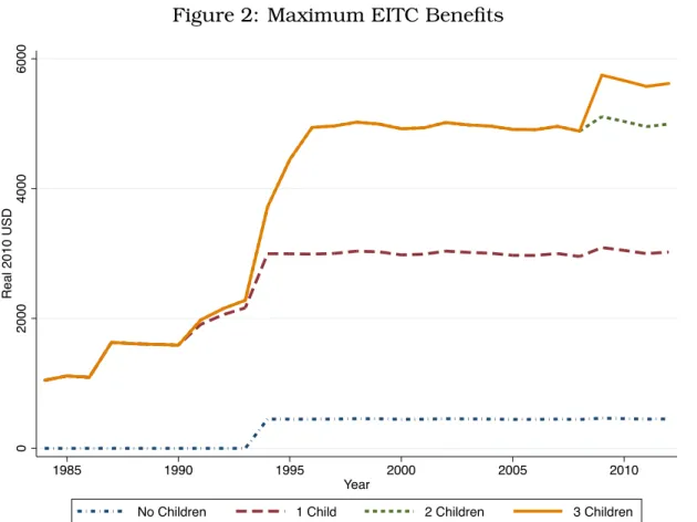
The amount of the credit initially increases with income, and is phased out at higher earnings levels. In addition to earnings, the credit is de-termined by the number of dependent children in the tax filing house-hold. Figure 1 displays the federal EITC schedule for various years, re-flecting some of the expansions over the previous thirty years. Some of the EITC expansions created differential changes to the maximum benefit

lev-2_{http://www.eitc.irs.gov/EITC-Central/eitcstats}

(18)

els across the number of children in the household. Figure 2 displays the evolution of the maximum benefit by the number of children in the house-hold. Notice that up until the early 1990s benefits were not dependent on the number of children (beyond one); by the mid 1990s households with two or more children were eligible for substantially higher credits than families with one child. In the late 2000s families with three or more chil-dren became eligible for higher benefits than families with two chilchil-dren.

Beyond the EITC, income taxes and child tax credits also determine federal tax liability. The child tax credit was created in the Taxpayer Relief Act (TRA) of 1997. Initially the credit was for $400 per qualifying child. The credit was increased in phases and as of 2015 the maximum credit is $1,000 per qualifying child. As income passes a threshold ($75,000 in 2015) the credit is phased out $50 for each additional $1,000 of in-come. Currently 15% of income over $3,000 is refundable. Individuals with income below $3,000 do not receive the child tax credit3_{. The rules}

have changed since 1997, but the magnitude of these changes are much smaller than the EITC expansions. A third important piece of the federal tax code is the income tax. The bounds of the brackets are adjusted for inflation and marginal tax rates have changed very little for low income individuals over the past 30 years. Furthermore, while changes to EITC and child tax credits differentially affect mothers depending on the num-ber of children she has, changes in income taxes do not differentially affect mothers across any observable (like number of children). The inclusion of year fixed effects in an empirical specification will absorb the time varying

(19)

aspect of income taxes. Changes to the EITC program represent the vast majority of the changes in tax liability, especially for low income single women.

2.2 State Taxes

State taxes vary both across state and within state, across time. State tax liability is primarily determined by income tax, EITC supplements and in a small number of states child tax credit supplements and rent or home-owners credits. The largest changes in state tax policy have been in the form of state EITC supplements. State EITC programs work much the same as federal EITC program; low income workers receive a supplement to their wages, on top of what the federal EITC program provides. Twenty-five states and the District of Columbia have implemented state EITC pro-grams. Implementation dates range from 1986 (Rhode Island) to 2015 (California). Figure 3 is a chart of the state EITC implementation dates. Implementation across states has been steady since the mid-1980s. Most of the EITC supplemental programs are disbursed as a percentage of the federal EITC value and are typically refundable (as is the federal EITC). State income taxes are another source of cross-state variation in post-tax income. For single filers with $25,000 in taxable income in 2015 marginal tax rates range from zero in seven states to nearly 8% in Maine4_{. As of}

2015, only five states have child tax credit supplements paid as either a percent of the federal child tax credit or as a fixed amount.

4

http://taxfoundation.org/article/state-individual-income-tax-rates-and-brackets-2015

(20)

2.3 AFDC/TANF

Prior to 1996, Aid to Families with Dependent Children (AFDC) made up the bulk of what is often referred to as welfare in the United States. Created as a part of the Social Security Act of 1935, AFDC provided cash payments most often to low-income single mothers. Monthly benefits are maximum at zero income, and are phased out after an income disregard. The effective phase out rate depends on how low long an individual has had positive income. States are allowed to set maximum benefit levels but the income disregard and phase out rates were federally standardized. Figure 4 shows a typical AFDC schedule an individual would face when enrolling in AFDC.

By the mid-1990s, over 14 million individuals – or five percent of the population – depended on AFDC payments that totaled over $22 billion in nominal terms5_{. With phase out rates as high as 100%, critics of AFDC}

suggest that the program creates a strong disincentive for mothers to join the workforce. McKinnish, Sanders, and Smith (1999)estimate effective av-erage tax rates of 35 to 40% for AFDC recipients over the years 1988-1991, exceeding marginal tax rates for the top income bracket (28-31 percent) over the same years 6. Employment rates measured around 60 percent among single mothers between 1992 and 19957.

Partially as a response to the low employment participation of AFDC eligible individuals and an increase in recipiency, many states applied for 5_{Department of Health and Human Services, Indicators of Welfare Dependence Annual}

Report to Congress 2008. Accessible at http://aspe.hhs.gov/report/indicators-welfare-dependence-annual-report-congress-2008

6_{http://www.taxpolicycenter.org/taxfacts/displayafact.cfm?Docid=543} 7_{Tabulation from the Current Population Survey.}

(21)

and were granted waivers to the federal program, increasing program flex-ibility in an effort to encourage work and reduce caseload. The earliest waivers were implemented in 1992 and by 1996 over half of the states had implemented an approved program8_{. In 1996 the US government}

passed the Personal Responsibility and Work Opportunity Reconciliation Act (PRWORA). PRWORA replaced AFDC with Temporary Assistance for Needy Families (TANF), a program that created time limits and work re-quirements for many single mothers seeking assistance. Stated goals of the PRWORA include “end[ing] the dependence of needy parents on govern-ment benefits by promoting job preparation, work, and marriage”.9 _Like

many of the AFDC waivers that preceded, TANF afforded states much more flexibility in of terms eligibility requirements, time limits and the benefit calculation formula. Figure 5 shows a sample of four states that selected very different benefit schedules by 1998. In general, states do not adjust benefit levels for inflation annually, and though discrete increases in bene-fits occur irregularly, the real value of TANF benebene-fits has eroded over time. In the five years following the passage of PRWORA, the number of families receiving income assistance from TANF fell from 4.5 million to 2.2 million. Welfare reform was largely perceived as a success as caseloads fell while consumption levels remained constant or perhaps even increased through the early 2000s (Meyer and Sullivan 2004, 2008).

8_For _details _see

http://aspe.hhs.gov/basic-report/state-implementation-major-changes-welfare-policies-1992-1998

9_{Personal Responsibility and Work Opportunity Reconciliation Act of 1996. Accessible}

at http://www.gpo.gov/fdsys/pkg/PLAW-104publ193/html/PLAW-104publ193.htm

(22)

2.4 Supplemental Nutrition Assistance Program

Supplemental Nutrition Assistance Program (SNAP), formerly known, and commonly referred to as Food Stamps, is a federal program providing additional resources to low income individuals with the requirement that the benefits be used to purchase food. Implementation of the food stamp program began state by state, beginning in the mid 1960s. By 1974 the program was operating nationwide. Originally, benefits were disbursed as physical coupons to the recipients. During the 1990s many states went to electronic benefit transfer (EBT) cards. As part of the PRWORA, states were required to use EBT for disbursement of SNAP benefits by October 1, 2002. The maximum benefit is allotted to families with no income. For families with income, benefits are reduced by 30 cents for each dollar of in-come after deductions. There is also an additional percentage disregard for earned income, as of 2015 workers could deduct 20 percent of earnings.

SNAP benefits are adjusted for inflation annually. Over time there have been a few incremental increases, beyond inflation adjustment, to the SNAP benefit levels. For the empirical Section of this paper I will not be able to identify a labor response from adjustments to SNAP due to lack of policy variation. However I do include SNAP benefits in the analysis due to important interactions with AFDC and TANF. Unlike EITC benefits, which do not interact with SNAP, AFDC and TANF benefits count as unearned income against SNAP benefits. Each additional dollar of AFDC or TANF an individual receives reduces their SNAP benefit by 30 cents. While this does create cross-state variation in effective SNAP benefits, the variation is collinear with state AFDC or TANF policy. AFDC/TANF and SNAP are

(23)

also linked in terms of receipt, many states have a common application and benefits are typically disbursed to the same EBT card. Users spend money from one program or another by entering a program specific PIN at the point of transaction. I discuss how I control for the direct interaction of SNAP and AFDC/TANF in Section 4.

3 Theoretical Framework 3.1 General Framework

In this section I develop a simple model of the labor supply decision for low income single women. This is a simple static model that only con-siders the extensive margin, the discrete choice whether or not to work. I make this simplifying assumption because the literature suggests that single women respond to work incentives more along the extensive mar-gin than the intensive marmar-gin (Heckman, 1993, Meyer and Rosenbaum, 2001a, Eissa and Liebman, 1996). If the individual works, they will receive their potential earnings net of taxes, and transfers. If the individual does not work, earnings are zero but they receive income in the form of trans-fers. The individual does not choose the number of hours worked, or the levels of income conditional on work, they simply observe their potential income separately from all sources and choose their employment status. Individuals in the model also have an unobserved distaste for work. Utility

(24)

for individual i is defined most generally in the following way: U_i = 8 > > < > > : uiw =u(yi1w,yi2w, ...yiPw) ci if working (w) uin =u(yi1n,yi2n, ...yiPn) if not working (n)

where l equals 1 if individual i chooses to work and zero if not. ypw is in-come from source pwhen the individual works (i.e. net federal tax liability) and ypn is the income from source p when not working. u(·) is the utility the individual obtains from income sources. c_i is the utility cost of work-ing for individual i, unobserved by the researcher. However, I assume c_i is a function of observable characteristics plus an unobserved idiosyncratic component:

c_i = f(X_i) +#_i

where X_i is the vector of observables and#_i is the idiosyncratic component. Given this framework, an individual will choose to work if their distaste for work is sufficiently small, specifically when:

#_i <u(y_i1w,yi2w, ...yiPw) u(yi1n,yi2n, ...yiPn) f(Xi)

Changes to the income sources will induce individuals at the margin to enter or exit the workforce.

3.2 Heterogeneous Effects

I begin with the simplifying assumption that there are no income ef-fects by assuming linear utility. When I actually estimate the labor supply

(25)

function I explore a parameterization that allows for income effects. The hypothesis I will test is whether workers react differently across forms of income. By introducing individual parameters for each income source, p_p, I allow that each can have differential effects on utility, and therefore behavior. Utility takes the form:

U_i = 8 > > < > > : ÂP_p=1ppyipw a·Xi #i if working (w)

ÂP_p=1ppyipn if not working (n)

(1)

where pp is the effect that income source p has on utility. Now individuals choose work when:

#_i <

P

Â

p=1

p_p y_ipw y_ipn a_·X_i (2)

where ypw ypn is the change in income from source p by moving from non-employment to employment. Again, the individual will choose to work only if their idiosyncratic realization of #_i is sufficiently small. Total labor supply will depend on where, in the distribution of#, the value of the right hand side of equation (2) lies. The probability an individual works (and rate of employment) is:

F

Â

P

p=1

p_p y_ipw y_ipn a_·X_i

!

(3) where F is the CDF of the distribution from which#_i is drawn.

(26)

4 Data

The data I use for the estimation come from the Current Population Survey (CPS) via the Integrated Public Use Microdata Series10_{. The CPS is}

the main source of labor market statistics in the United States and con-tains contemporaneous work status at the individual level as well as basic demographic information. Each household in the CPS is surveyed a total of eight times: two sets of four consecutive months separated by an eight month gap. Individuals being surveyed for the fourth consecutive month (surveys four and eight) comprise the outgoing rotation group (ORG). In March of every year, households are asked an additional set of questions. Importantly, the March supplement contains data on individual’s earnings from the previous calendar year. For the purposes of this exercise I focus on single women age 18 to 55 with less education than a bachelor’s degree, who are not in the military or enrolled full time in school. I focus on this subset of the population because they are most affected by income sources described in Section 2. The data I use for the estimation spans 1984-2011 (ORG data are limited to 1996-2010).

I created a benefit calculator to approximate the AFDC, TANF and SNAP benefits an individual is eligible for using rules provided by the Urban Institute. AFDC and SNAP rules come from the TRIM311 program rules database, and TANF rules are detailed in the Welfare Rules Database12_.

AFDC and TANF rules are quite complicated and I have to make some sim-plifying assumptions. Some of the income disregards in the AFDC/TANF

10_{Ruggles, Genadek, Goeken, Grover, and Sobek (2015)} 11_{http://trim3.urban.org/}

(27)

benefit formula change over time; for calculation purposes I use the for-mula that is in effect as a person initially enters the program. I assume that single mothers are eligible for AFDC/TANF in terms of asset tests, have not reached their time limit and have no income other than wage earnings. To calculate federal and state tax liabilities I use the NBER’s TAXSIM913 module for STATA. TAXSIM9 takes the tax year, household composition and income as inputs and calculates tax liabilities or credits separately by federal and state. I assume the woman files her taxes as head of the household, she claims her children as dependents and has no income other than wage earnings.

The framework laid out in Section 3 requires the researcher to observe disaggregated sources of income for each individual if they are working and if they are not working. Given wage earnings and demographics I can calculate the composite sources of income as stated above. To calculate income sources when an individual does not work I assume wage earnings (and total income) are zero. Calculating the income sources of those for whom I do not observe wage earnings is more difficult. I only observe wage earnings for the those that report positive annual earnings in the March CPS. I do not observe potential wage earnings for those that are not working or for any individuals in the ORG. To estimate potential earnings for individuals who report not working and for those not in the March CPS I impute wages based off of workers in the March CPS.

A second challenge is that I would like to identify work responses from policy changes alone. If the empirical wage distribution adjusts to policy

13_{http://users.nber.org/˜taxsim/taxsim9/}

(28)

then the income sources themselves are endogenous to the policy. As an example, suppose there were wage growth for a particular subset of the in-dividuals relative to the rest, inin-dividuals in that subset might move into the labor force because the payoff from working has increased. The increase in wages will also lead to higher a EITC benefit (if the potential incomes lie in the phase-in range), using the OLS imputed wages would introduce positive correlation between effective EITC benefits and employment, but not due to a policy change. I want to identify labor supply responses from policy changes alone, holding wages constant. To do this I construct a simulated instrument, described later in Section 4.2.

4.1 Earnings Imputation

To impute earnings, I begin with the set of observations that contain annual earnings data (women in the March CPS who reported working in the previous year) and estimate the following equation, separately by educational attainment (high school dropout, high school graduate and some college, but less than a degree) and year cells:

log(wi) = ds+w·Xi+#i (4)

In addition to state fixed effects ds, control variables within Xi include a quadratic function of age, dummy variables for race and ethnicity, and a categorical variable describing the individual’s residence location (i.e. urban, suburban, rural). I use the coefficient estimates from the state fixed effects and the vector of demographics to predict log wages for all

(29)

individuals in the sample, whether I observe earnings or not, to keep the specification consistent across all individuals. EissaLiebman1996

Given an imputed income along with the state of residence, year and household size provided in the CPS, I am able to approximate net tax lia-bility using TAXSIM and welfare benefits using the TANF/AFDC and SNAP calculator I created.

4.2 Simulated Instrument

I want to identify labor supply responses from policy changes alone, not from the evolution of the wage distribution. To do so, I construct a simu-lated instrument in the spirit of (Currie and Gruber, 1996). The idea is to fix the income distribution and calculate the evolution of income sources due to policy changes alone. The simulated instrument is constructed in several steps. First I aggregate all individuals in the CPS that report an-nual income (those who report working in the March CPS) and construct a distribution of real wages, adjusted for inflation using the Consumer Price Index for All Urban Consumers14_{. Second I calculate the points in the}

distribution of real income that bound each centile. Third, separately by education group, I calculate the percentage of individuals in each centile. High school dropouts will have higher mass in the lower centiles relative to high school graduates and vice versa, but the sum of the percentages across centiles for each education group is one. These percentages will be used as weights later. Fourth, separately by year, I calculate a mean nom-inal income level conditional on being within each of the centile bounds of

14_{From the Federal Reserve Economic Database, series CPIAUCSL}

(30)

the aggregate real distribution from Step 2. Fifth, for the mean nominal income level associated with each centile I calculate taxes and transfers separately by state, year and number of children. Finally, for each educa-tion group, year, state, number of children I construct a weighted average for each income source using the weights in Step 3. I now have an average potential income associated with each source that is weighted by a static income distribution, specific to an education level for each state, year and number of children. I merge these income sources onto the CPS data and use them as instruments for the income sources generated from imputed income above.

Table 1 displays summary statistics for the simulated instrument. EITC credits are highest for those with the lowest income because more of them fall into the income eligibility range than those with a higher education whose earnings are more often in the EITC phase-out portion of the distri-bution or higher. State taxes are, on average, a liability for each education group but smaller for those with lower income. Benefits, in the form of AFDC/TANF and SNAP are highest for low education mothers. The last two rows combine all of the programs. Women with two children and a high school diploma or less education average net transfers, while child-less mothers and college educated mothers of two average net tax liability when working. Figure 7 shows where the variation in each of the instru-ments comes from. Each variable is measured as a net increase in income due to employment, from indicated source. All of the graphs represent the simulated instrument for high school dropouts and are denominated in thousands of real dollars. A value of 1 means that becoming employed nets

(31)

the individual $1,000 from the income source. The left panel of each set separates the variables by number of children. The right panel separates variables across a selection of states, and displays values for a mother of two children. Work incentives from all three programs have increased over time. The change in incentives has been more extreme for mothers than non-mothers, especially for federal and state taxes. The right panels show that while there is no cross-state variation in federal taxes, there is con-siderable cross-state and within-state cross-time variation in state taxes and AFDC/TANF.

5 Estimation

5.1 Aggregating the Budget Set

Each of the income support programs considered in this paper affects the budget set individuals face at the low end of the income distribution. Figure (6) shows how all of the sources of income interact. This specific collection of budget sets illustrate how I will test the main hypothesis. All of these budget sets are for single mothers with two children in the state of Ohio. The top graph is for 1992; the black line is the 45 degree line. When there are no taxes or transfers pre-tax income equals post-tax income and the budget set is the 45 degree line. The dot-dashed blue line is the budget set when we include AFDC or TANF. Notice there is a transfer of about $6,000 in AFDC or TANF for those with zero pre-tax income. As income increases the AFDC/TANF line gets closer to the 45 degree line due to the phase out. The dashed red line traces out the budget

(32)

set if we consider both SNAP (conditional on AFDC/TANF income) and AFDC/TANF. Transfers at zero are even higher but the effective marginal tax rate is also very high. The green dashed line adds state taxes to AFDC and SNAP. Finally the solid orange line incorporates all adjustments to income including federal and payroll taxes. EITC and child tax credits push the budget set higher and reduce the marginal tax rate. This is the aggregate budget set.

The middle graph shows the budget set the same mother would face three years later, after an EITC expansion. The AFDC and SNAP lines are essentially unchanged, but the budget set pivots up due to the EITC. The third graph is two additional years later, in 1997. As Ohio transitioned from AFDC to TANF they changed the phase out rate, effectively pivoting the budget set up again. The change from the top to the middle graph increases gains from employment for low income single mothers through the EITC. The change from the middle to the bottom affects the aggregate budget set in the same way, but due to a change in AFDC/TANF. My hy-pothesis is that while these two changes may have had differential impacts on labor supply even though they had similar effects on the envelope of all income sources.

5.2 Estimating Equation

I begin with a linear approximation of the labor supply equation (3), later I will control for income effects. I collapse the data down to a cell defined by state, year, education group and number of children: the level of policy variation. The percent of sample women in a given cell that are

(33)

employed is: L_s,y,e,k = P

Â

p=1 pp ypw y_{pn s}_,_y_,_e_,_k+aXs,y,e,k+ds+ty+ei (5)

where (ypw ypn)s,y,e,k is the average change in income from source p when a single woman in state s, and year y, with education e, and k number of children moves from not working to working. X_s,y,e,k is a vector of demo-graphic and other controls including cell averages for age and age squared, controls for race ethnicity and state unemployment, fixed effects for num-ber of children, educational attainment, year, month and CPS division15. The vector also includes the number of children that would not be eligi-ble for medicaid if the mother earned her imputed wage16_{. It is difficult}

to place a monetary value on medicaid benefits so I do not interpret the coefficient in terms of an elasticity, but not including medicare eligibility changes could lead to omitted variable bias for the estimates of the other sources of income (if Medicare law changes are coincidental with state AFDC or TANF rules for instance).

For the estimation, I consider four sources of income (or liability): the federal tax code, the state tax code, AFDC or TANF benefits and SNAP. As discussed in Section 2, AFDC/TANF and SNAP interact in important 15_{CPS divisions are geographic groups of three to eight states. There are nine divisions}

in total: New England, Mid Atlantic, East North Central, West North Central, South Atlantic, East South Central, West South Central, Mountain, and Pacific. Using CPS division fixed effects controls for common shocks that affect geographic regions of the United States, while exploiting some cross-state variation in policy. A concern when not explicitly controlling for state fixed effects is that state legislation could be a reaction to the economic conditions within the state. Controlling for state unemployment is an attempt to ameliorate this concern. I also include state fixed effects as a robustness check below.

16_{These rules changes by state and year, I thank Hilary Hoynes for sharing the eligibility}

parameters.

(34)

ways. While there is insufficient policy variation to identify labor supply responses, I account for SNAP in two ways. First, I simply control for changes in SNAP (mostly induced by state AFDC or TANF changes). Sec-ond, I combine of AFDC/TANF and Food Stamp benefits and estimate a single labor supply response from the two programs.

I use two stage least squares, using the simulated income change from each program calculated at the cell level, described in Section 4.2, as an instrument for the average change in income calculated using the imputed earnings.

5.3 Results

Table 2 displays the results from estimating Equation (5). Each variable listed is the income increase from a given source if an individual were to change from non-employment to employment. For instance an increase in the federal taxes variable could arise from an expansion of the EITC. In this case, federal tax credits for working individuals would increase while taxes at zero income remain unchanged. The expected sign on each of the coefficient estimates is positive. All else equal, increasing the income gain from working should increase labor supply.

Column 1 shows the estimate of the labor supply response to a change in aggregate income when moving from non-employment to employment. This is a common method to generate the labor supply elasticity used to calibrate an optimal taxation model. For the first column I calculate the implied elasticity as:

(35)

h = ∂Ls,y,e,k ∂(Yw Yn)s,y,e,k · ¯ Yw Yn ¯ L

where (Yw Yn)s,y,e,k is the total change in income from employment for a given cell. (Yw ¯ Yn) is the average total income change across cells, Ls,y,e,k is the employment ratio at the cell level and and L¯ is the average employ-ment ratio across cells. The implied elasticity for total income, shown in the bottom panel, is 0.33 which is in line with much of the existing liter-ature (see Chetty (2012)). Column 2 displays the results when I allow for heterogeneous effects across income sources. The implied elasticities for columns 2-4 are calculated as:

h_p = ∂Ls,y,e,k ∂(ypw ypn)s,y,e,k · ¯ Yw Yn ¯ L

where (ypw ypn)_s,y,e,k is the income change from source p for a given cell. The interpretation is a one percent change in total income due to a change in source p induces an hp percent change in the employment ratio. The results in Column 2 suggest labor responses from changes in the federal tax code, and across states, within a division, appear greater than the responses associated with changes to income from AFDC or TANF. In the bottom panel, the c2 and p-value listed are associated with a test that the three coefficients are equal. The hypothesis can be rejected, suggesting the responses are indeed different across programs. The differences between Columns 1 and 2 are also important for optimal tax theory, using only the labor supply elasticity of total income to calibrate a model could be misleading.

(36)

In Column 2, I estimate a labor supply response for AFDC or TANF and control for SNAP separately. In Column 3, I combine the two programs and measure net effects of changes to AFDC or TANF and Food Stamps. I do this because of the interactions of the programs described in Section 2. Combining the programs does not meaningfully change the results. The implied elasticities from changes to AFDC or TANF and SNAP remain much smaller than elasticities coming from the tax code.

Finally, in Column 4, I introduce an indicator variable that equals one for each year after TANF replaced AFDC (beginning in 1997)17_{. I interact}

the dummy with the ”AFDC/TANF and SNAP” variable to allow for a differ-ential effect across AFDC and TANF. In this column, the estimate labeled ”AFDC/TANF and SNAP” is the estimate for only the AFDC regime. The estimate labeled TANF and SNAP is the interaction with the time dummy. The sum of the last two estimates is the estimated elasticity for the TANF regime. There are many reasons to believe labor supply responses may be different across these two welfare regimes. States adjusted eligibility rules, work requirements, time limits and other parameters. Empirically, however, the labor supply response across the two programs are indistin-guishable; the interaction term is essentially zero.

That the labor responses to federal taxes and state taxes are quite sim-ilar across specifications is an interesting result. The source of variation from federal taxes is largely due to EITC expansions, a program that even claimants do not usually display an understanding of the details (Romich and Weisner, 2000). While much of the variation at the state level is due 17_{I have also used an indicator variable equal to one for an AFDC waiver and TANF, the}

(37)

to cross-state income tax variation.

Table 3 displays a set of robustness checks using different geographic fixed effects. Column 1 in Table 3 is the same as Column 4 in Table 2 and is provided for comparison. Table 3 Column 2 replaces division fixed effects with state fixed effects. Column 3 replaces division fixed effects with region fixed effects, a coarser geographic grouping of states. Columns 4 - 6 interact geographic fixed effects with the year fixed effects. Estimates for federal taxes and AFDC/TANF and SNAP are robust to the choice of geographic fixed effects. However controlling for state fixed effects absorbs the identifying variation; estimates on state taxes are essentially zero. This suggests that most of the labor supply response from the state tax code comes from cross-state level differences in income taxes as opposed to within-state changes to EITC supplemental programs.

One may be concerned that if federal and state taxes tend to affect different portions of the income distribution than AFDC/TANF and Food Stamps, differences in estimated labor supply responses could simply be due to income effects. The parameterization in equation (3) does not allow for income effects, implying a vertical shift of the budget set will lead to the same labor supply. In Table 4, I control for income at zero earnings to allow for income effects. It might be important to control for each source of income at zero earnings, except AFDC/TANF and SNAP account for es-sentially all of the income for non-workers. Each column is analogous to those in Table 2. The sign on the total income at zero earnings is negative, as expected, small and marginally significant. A vertical shift in the bud-get set should lead to a lower labor supply. The inclusion of fixed effects

(38)

slightly reduces the elasticity estimates, but in a uniform way, suggesting income effects may be important, but are not driving the differences in labor supply responses across programs.

6 Policy Implications

In Section 5, I provided evidence that labor supply reacts to a greater degree to adjustments in work incentives derived from the tax code com-pared to changes in the (dis)incentives provided by welfare-type programs. In this section I will discuss what the findings mean in terms of policy.

I want to be clear about the limitations of the policy implications one can glean from the results in presented in Section 5. First I do not estimate the effect that changes to a program’s parameters have on the recipiency rate of the program. While effects on recipiency do not affect estimation of the elasticity of labor supply, it is important from an accounting stand-point, or for cost-benefit analysis. For example, if the benefit levels are increased for a particular program, the costs of the program increase for two reasons: directly from the increase in benefit levels for the current recipients, and indirectly due to an increase in recipients who now claim the benefit that did not prior to the increase. Second, the results in Sec-tion 5 are not sufficient to make claims about general equilibrium effects. Specifically an increase in benefits for a particular program or a decrease in taxes must be financed. To the extent that the burden of the financing derives from tax increases to married women, men, or higher educated in-dividuals, the results in Section 5 describe an incomplete description of the effect of increasing transfers to single women. For example, suppose taxes

(39)

were increased on higher educated individuals to finance an increase in benefits to low income individuals. The results do not describe the change in labor supply for the higher educated due to higher taxes, which would be important to consider when designing policy.

Instead of providing a social welfare function, in this section I will high-light two potential policy goals and discuss what the above results suggest about attaining those goals.

Policy Goal 1: Increase Employment/Decrease Non-employment

Suppose the goal of the social planner is to induce non-employed to seek employment among those with low earnings potential. The social planner has two options: decrease transfers to the non-employed or in-crease transfers to low income workers.

First consider reducing transfers to the non-employed. Implementing this policy through the tax code is likely not feasible, the tax code currently provides no resources to the non-employed so reducing aggregate transfers would take the form of tax liability on those who have no earnings. Alter-natively the planner could reduce benefits from welfare-type programs to the non-employed. Given the estimates from Section 5 one would expect the labor supply response from this type of measure to be relatively small and at the expense of the utility of the recipients of the transfers. However decreasing the benefits would not require any outside financing, and in fact would save government resources.

Suppose instead the social planner decided to increase benefits for low wage workers. This policy could be implemented through an EITC

(40)

sion/income tax reduction or through a reduction in the phase out rate of TANF or SNAP. My estimates suggest that increases to EITC and other tax parameters would induce more people to seek employment than an equivalent phase-out rate adjustment to the welfare-type programs.

Policy Goal 2: Transfer Resources to Non-employed

Suppose the goal of the social planner is instead to transfer resources to the non-employed while minimizing distortion to the labor market. The social planner again has at least two options: increase the benefits to the non-employed or shift the entire budget set upwards.

Increasing the benefits to the non-employed could be accomplished through the tax code. While there are currently no refundable tax credits to those with no earnings, it seems more feasible to extend tax credits to the non-employed than to levy taxes. However, my estimates suggest that increasing benefits in the tax code would lead to a relatively large labor supply reduction. An increase in the benefits through the welfare-type programs, on the other hand, would elicit a smaller reduction in labor supply. However, since the recipiency rates of TANF and SNAP is smaller than that of the EITC, a welfare-type benefit increase would reach fewer individuals.

Alternatively the social planner could increase transfers to low income workers as well as the non-employed. This could be done through either the tax code or welfare-type programs. The benefit of this policy is that it would minimize the reduction in labor supply, as suggested by the esti-mates of the income effect in Table 4. The drawback of this policy option is,

(41)

of course, that it is the most costly of the options facing the social planner. One takeaway is that US policymakers implemented policy in a man-ner consistent with the analysis of the two objectives above. AFDC and SNAP were largely designed to transfer resources to low or no income fam-ilies. The institutional framework surrounding these programs limited the distortionary effect on the labor market as evidenced by the estimates in section 5. On the other hand, the EITC was designed with the goal of in-creasing labor supply. The larger labor supply elasticity is consistent with this type of program’s effectiveness.

7 Conclusion

In this paper, I consider four major sources of income support: fed-eral taxes and credits, state taxes and credits, AFDC/TANF and SNAP. I separately and simultaneously estimate the labor supply effects of multi-ple overlapping income support programs. Using a simulated instrument strategy, I identify labor supply responses solely off of policy changes. I estimate that the labor force response to changes in the benefits adminis-tered through the tax code is larger than the response to changes in more traditional welfare programs like AFDC, TANF and SNAP. The differential responses suggest that the budget set faced by the labor force is more than just the sum of its parts. Identical budget sets comprised of different un-derlying programs can lead to different labor supply and welfare outcomes. Many models of taxation optimize the shape of the aggregate budget with estimates of the labor supply elasticity without independent consideration of the underlying programs. The estimates of this paper suggest that

(42)

counting for the differences in elasticities across programs is important. There are several limitations to the analysis that should be addressed in future work. Capturing all of the elements of the income support programs is challenging, especially after the 1996 welfare reform, and few empirical papers have attempted to do so. Including more of the state level policy variation may prove important. Analysis of labor response along the in-tensive margin could provide a more complete description of how the labor force responses to income programs. Finally, a theoretical model of tax-ation that considered multiple programs each with different labor supply responses could help explain how the results of this paper affect optimal policy.

(43)

Figure 1: EITC Benefits 0 5000 10000 15000 20000 25000 30000 35000 0 500 1000 1500 2000 2500 3000 3500 4000 4500

EITC Benefits

Single Mother, 2 Children

1986 1987 1991 1994 1997

Earnings

R

ea

l 2

00

0

U

S

D

Notes: Each line describes the federal earned income tax credit for a different year.

(44)

Figure 2: Maximum EITC Benefits 0 2000 4000 6000 R e a l 2 0 1 0 U SD 1985 1990 1995 2000 2005 2010 Year

No Children 1 Child 2 Children 3 Children

Maximum Annual EITC benefit

Notes: Each line describes the federal Earned Income Tax Credit for an individual whose earned income qualifies them for the maximum benefit level.

Figure 3: State EITC Implementation

Sheet3 MA RI MD VT WI IA MN NY OR KS 1986 1987 1988 1989 1990 1991 1994 1997 1998 DC IL CO ME DE LA IN NJ OK VA NE NM MI CT OH CA 1999 2000 2002 2004 2006 2007 2008 2011 2013 2015 32

(45)

Figure 4: Example AFDC Schedule 0 100 200 300 400 500 600 700 800 900 1000 11 0 0 Mo n tl h y R e a l AF D C (2 0 1 0 U SD ) 0 500 1000 1500 2000 2500

Real Income (2010 USD)

1 Child 2 Children 3 Children

Monthly Real AFDC benefits

Single Taxfiler, State: Massachusetts, Year: 1994

Notes:This AFDC schedule assumes the single mother is both eligible and has no income other than wage earnings. Parameters of the schedule represent the AFDC rules faced when initially entering the program. The income disregards decrease after sustained earnings.

(46)

Figure 5: Example TANF Schedules 0 100 200 300 400 500 600 700 800 900 1000 11 0 0 Mo n tlh y R e a l T AN F (2 0 1 0 U SD ) 0 500 1000 1500 2000 2500

Monthly Real TANF benefits Single Taxfiler, State: California, Year: 1998

(a) California 0 100 200 300 400 500 600 700 800 900 1000 11 0 0 Mo n tl h y R e a l T AN F (2 0 1 0 U SD ) 0 500 1000 1500 2000 2500

Monthly Real TANF benefits Single Taxfiler, State: Deleware, Year: 1998

(47)

0 100 200 300 400 500 600 700 800 900 1000 11 0 0 Mo n tlh y R e a l T AN F (2 0 1 0 U SD ) 0 500 1000 1500 2000 2500

Monthly Real TANF benefits Single Taxfiler, State: Minnesota, Year: 1998

(c) Minnesota 0 100 200 300 400 500 600 700 800 900 1000 11 0 0 Mo n tl h y R e a l T AN F (2 0 1 0 U SD ) 0 500 1000 1500 2000 2500

Monthly Real TANF benefits Single Taxfiler, State: Wisconsin, Year: 1998

(d) Wisconsin

Notes: These TANF schedules assume the single mother is both eligible and has no income other than wage

earnings. Parameters of the schedule represent the TANF rules faced when initially entering the program. In some cases income disregards decrease after a period sustained earnings.

(48)

Figure 6: Example Aggregate Budget Sets (a) Ohio 1992 0 10000 20000 30000 40000 Po st -t a x In co me 0 10000 20000 30000 40000 Pre-tax Income

AFDC plus Food Stamps plus State Taxes

plus Fed/Payroll Taxes 45 degree line

Single Taxfiler, Dependent Children: 2, State: Ohio, Year: 1992

(b) Ohio 1995 0 10000 20000 30000 40000 Po st -t a x In co me 0 10000 20000 30000 40000 Pre-tax Income

AFDC plus Food Stamps plus State Taxes

(49)

0 10000 20000 30000 40000 Po st -t a x In co me 0 10000 20000 30000 40000 Pre-tax Income

TANF plus Food Stamps plus State Taxes

Single Taxfiler, Dependent Children: 2, State: Ohio, Year: 1997

(c) Ohio 1997

Notes: These budget sets assume the single mother has two children and is both eligible for AFDC/TANF and SNAP and has no income other than wage earnings. Parameters of the schedule represent the TANF rules faced when initially entering the program. In some cases income disregards decrease after a period sustained earnings. See Section 5.1 for more details.

(50)

Figure 7: Identifying Variation in Simulated Instrument

(a) Federal Taxes: Cross Child

-1 0 1 2 3 4 C h a g n e in F e d e ra l T a x W o rk In ce n ti ve 1985 1990 1995 2000 2005 2010 Survey year No Children 1 Child 2 Children 3 Children

Variation in Simluated Instrument for Change in Federal Tax Work Incentive

(b) Federal Taxes: Cross State

-1 0 1 2 3 C h a g n e i n F e d e ra l T a x W o rk In ce n ti ve 1985 1990 1995 2000 2005 2010 Survey year

California Florida Georgia Illinois

Michigan New Jersey New York North Carolina

Ohio Pennsylvania Texas Virginia

(51)

-. 3 -. 2 -. 1 0 .1 C h a g n e in St a te T a x W o rk In ce n tive 1985 1990 1995 2000 2005 2010 Survey year No Children 1 Child 2 Children 3 Children Variation in Simluated Instrument for Change in State Tax Work Incentive

(c) State Taxes: Cross Child

-1 -. 5 0 .5 C h a g n e i n St a te T a x W o rk In ce n tive 1985 1990 1995 2000 2005 2010 Survey year

California Florida Georgia Illinois

Michigan New Jersey New York North Carolina

Ohio Pennsylvania Texas Virginia

Variation in Simluated Instrument for Change in State Tax Work Incentive

(d) State Taxes:Cross State

(52)

-6 -4 -2 0 C h a g n e in AF D C /T AN F Be n e fit s 1985 1990 1995 2000 2005 2010 Survey year No Children 1 Child 2 Children 3 Children

Variation in Simluated Instrument for AFDC/TANF Benefits due to Employment

(e) AFDC/TANF: Cross Child

-6 -4 -2 0 C h a g n e i n AF D C /T AN F Be n e fit s 1985 1990 1995 2000 2005 2010 Survey year No Children 1 Child 2 Children 3 Children

Variation in Simluated Instrument for AFDC/TANF Benefits due to Employment

(f) AFDC/TANF: Cross State

Notes: Each of these graphs display the evolution of simulated instruments over time. These graphs show the values for high school dropouts. The left panels separates the values by number of children. The right panels separate by state and are shown for single mothers with two children. The value of the instrument is the increase in income by becoming employed. The vertical axis is denominated in thousands of real 2010 USD.

(53)

Table 1: Summary Statistics of Simulated Instrument

(1) (2) (3) (4)

Estimation High School High School Some

Sample Dropout Graduate College

Panel A: Demographics Age 34.1 33.6 33.9 34.5 No Children Percent 65.1 59.6 65.8 67.0 1 Child Percent 17.7 16.9 17.8 18.0 2 Children Percent 10.8 12.3 10.6 10.3 3+ Children Percent 6.3 11.2 5.8 4.7 Percent Black 21.0 24.7 21.5 18.7 Percent Hispanic 14.6 30.0 12.2 10.0

Panel B: Income, Taxes and Transfers (Real 2010 Dollars)

Imputed Pre-tax Wage Earnings 22452 14445 21819 26858

Federal Taxes: No Children 2093 874 1931 2772

Federal Taxes: 2 Children -972 -2046 -1120 -206

State Taxes: No Children 571 267 537 734

State Taxes: 2 Children 325 63 309 488

AFDC/TANF: No Children 0 0 0 0

AFDC/TANF: 2 Children 1666 2745 1546 1207

SNAP: No Children 605 982 594 462

SNAP: 2 Children 2213 3103 2199 1736

AFDC/TANF and SNAP: Zero Income, No Children 2052 2038 2051 2059

AFDC/TANF and SNAP: Zero Income, 2 Children 11439 11513 11402 11441

Net Tax and Transfers(T_i): No Children 5495 2351 5185 7127

Net Tax and Transfers(T_i): 2 Children -1156 -5640 -1242 1427

Number of observations 773367 138766 334359 300242

Notes: This table summarizes the simulated instrument. Each of the tax and transfer variables are

an average over a constant earnings distribution. The Imputed Pre-tax Wage Earnings is the weighted mean of the imputed incomes. A negative tax value is a tax credit. See Section 4.2 for details on the construction of the simulated instrument.

(54)

Table 2: Marginal Effects: Income Gain from Employment, Multiple Sources (1) (2) (3) (4) D y: Total Income 0.021 (0.0024)⇤⇤⇤ D y: Federal Taxes 0.045 0.041 0.038 (0.0052)⇤⇤⇤ _(0.0047)⇤⇤⇤ _(0.0053)⇤⇤⇤ D y: State Taxes 0.039 0.032 0.031 (0.018)⇤⇤ _(0.015)⇤⇤ _(0.015)⇤⇤ D y: AFDC/TANF 0.022 (0.0027)⇤⇤⇤

D y: AFDC/TANF and SNAP 0.019 0.020

(0.0024)⇤⇤⇤ _(0.0025)⇤⇤⇤

D y: TANF and SNAP -0.0018

(0.0019) N 16605 16605 16605 16605 r2 0.34 0.26 0.29 0.30 TotInc elast 0.33 fed elast 0.72 0.65 0.62 state elast 0.62 0.52 0.50

AFDC TANF elast 0.36

AFDC TANF SNAP elast 0.31 0.32

TANF SNAP elast 0.29

CraggDonald F 10568.8 304.8 1633.6 1009.2

Chi2 16.6 16.2 18.6

Pvalue 0.00024 0.00030 0.00033

Notes: (* P<.1, ** P<.05, *** P<.01). Standard errors clustered at the state level. The unit of observation is a state-year-educationGroup-numberKids cell. Regressions control for race, ethnicity as well as education, state, year and number of children fixed effects. Column 2 includes controls for SNAP. Column 3 estimates the joint effect of AFDC/TANF and SNAP, in addition to taxes. Column 4 introduces a dummy equal to one for every year after TANF was implemented in 1997. The fifth row of Column 4 is the estimate for AFDC and SNAP, the sum of the fifth and sixth rows is the estimate for TANF and SNAP. Implied elasticities are calculated the percent change in the employment ratio as a percent change in total income due to a change in the labeled source. See Section for details. The Cragg-Donald F-stat is a test for weak instruments with multiple endogenous variables. The c2 and p-values are from a test that all of the listed coefficients are equal.

(55)

Table 3: Marginal Effects: Income Gain from Employment, Multiple Sources: Robustness

(1) (2) (3) (4) (5) (6)

Division FE State FE Region FE Div x Yr FE St x Yr FE Reg x Yr FE

Dy: Federal Taxes 0.038 0.037 0.037 0.039 0.040 0.037

(0.0053)⇤⇤⇤ _(0.0051)⇤⇤⇤ _(0.0053)⇤⇤⇤ _(0.0056)⇤⇤⇤ _(0.0059)⇤⇤⇤ _(0.0053)⇤⇤⇤

Dy: State Taxes 0.031 -0.010 0.029 0.028 -0.033 0.027

(0.015)⇤⇤ _(0.014) _(0.015)⇤ _(0.015)⇤ _(0.016)⇤⇤ _(0.016)⇤

Dy: AFDC and SNAP 0.020 0.019 0.017 0.019 0.020 0.017

(0.0025)⇤⇤⇤ _(0.0024)⇤⇤⇤ _(0.0022)⇤⇤⇤ _(0.0026)⇤⇤⇤ _(0.0026)⇤⇤⇤ _(0.0022)⇤⇤⇤

Dy: TANF and SNAP -0.0018 -0.0022 -0.0023 -0.0017 -0.0011 -0.0020

(0.0019) (0.0017) (0.0017) (0.0019) (0.0020) (0.0017)

N 16605 16605 16605 16605 16605 16605

r2 0.30 0.32 0.30 0.31 0.37 0.30

fed elast 0.62 0.60 0.59 0.63 0.64 0.60

state elast 0.50 -0.16 0.46 0.45 -0.53 0.43

AFDC TANF SNAP elast 0.32 0.30 0.27 0.31 0.32 0.27

Notes: (* P<.1, ** P<.05, *** P<.01). Standard errors clustered at the state level. Column 1 is a reproduction of Table 2,

Column 4, for comparison. Column 2 replaces CPS division fixed effects with state fixed effects. Column 3 replaces CPS division fixed effects with CPS region fixed effects. Column 4 replaces CPS division fixed effects with division x year fixed effects. Column 5 replaces CPS division fixed effects with state x year fixed effects. Column 6 replaces CPS division fixed effects with CPS region x year fixed effects.

(56)

Table 4: Marginal Effects: Income Gain from Employment, Multiple Sources (1) (2) (3) (4) D y: Total Income 0.015 (0.0022)⇤⇤⇤ D y: Federal Taxes 0.043 0.038 0.037 (0.0052)⇤⇤⇤ _(0.0047)⇤⇤⇤ _(0.0054)⇤⇤⇤ D y: State Taxes 0.038 0.031 0.030 (0.018)⇤⇤ _(0.014)⇤⇤ _(0.014)⇤⇤ D y: AFDC/TANF 0.020 (0.0027)⇤⇤⇤

D y: AFDC/TANF and SNAP 0.016 0.016

(0.0022)⇤⇤⇤ _(0.0022)⇤⇤⇤

D y: TANF and SNAP -0.0016

(0.0018)

Income at Zero Earnings -0.0072 -0.0040 -0.0047 -0.0045

(0.0026)⇤⇤⇤ _(0.0025) _(0.0025)⇤ _(0.0025)⇤ N 16605 16605 16605 16605 r2 0.34 0.27 0.30 0.30 TotInc elast 0.25 fed elast 0.70 0.62 0.59 state elast 0.61 0.50 0.49

AFDC TANF elast 0.32

AFDC TANF SNAP elast 0.25 0.26

TANF SNAP elast 0.24

CraggDonald F 8748.2 273.1 1359.0 887.2

Chi2 19.5 20.0 22.0

Pvalue 0.000057 0.000045 0.000066

Notes: (* P<.1, ** P<.05, *** P<.01). Standard errors clustered at the state level. This table is analogous to Table 2, with the inclusion of a variable for the income an individual would receive if they had not earnings. The unit of observation is a state-year-educationGroup-numberKids cell. Regressions control for race, ethnicity as well as education, state, year and number of children fixed effects. Column 2 includes controls for SNAP. Column 3 estimates the joint effect of AFDC/TANF and SNAP, in addition to taxes. Column 4 introduces a dummy equal to one for every year after TANF was implemented in 1997. The fifth row of Column 4 is the estimate for AFDC and SNAP, the sum of the fifth and sixth rows is the estimate for TANF and SNAP. Implied elasticities are calculated the percent change in the employment ratio as a percent change in total income due to a change in the labeled source. See Section for details. The Cragg-Donald F-stat is a test for weak instruments with multiple endogenous variables. Thec2 and p-values are from a test that all of the listed coefficients are equal.

(57)

Part II

Optimal Income Taxation with Unemployment and Wage Responses: A Sufficient Statistics Approach (Joint work with Kory Kroft,

Etienne Lehmann and Johannes Schmieder) 8 Introduction

Recent decades have witnessed a large shift in the U.S. tax and transfer system away from welfare towards in-work benefits. In particular, for sin-gle mothers, work incentives increased dramatically: welfare benefits were cut and time limits introduced, the Earned Income Tax Credit (EITC) was expanded and changes in Medicaid, job training programs and child care provision encouraged work. The shift away from programs featuring a Neg-ative Income Tax (NIT) structure (lump-su