Forecasting model of tasks execution in the public transport system

Logistyka 4/2014

Krzysztof Bojda1

Wrocław University of Technology

Forecasting model of tasks’ execution in the public

transport system

Introduction

The departures’ punctuality achieved by vehicles operating the transport tasks is one of the most important criteria to evaluate the functioning of the public transportation system. Due to several conditions and external extortions it is unfortunately not always possible to provide the timetable in a form which will take into account every possible planned disturbances (like e.g. construction works), as well as any undesired events arising on random character (e.g. traffic congestion). However, the increasing availability of operational data describing the execution of transport tasks allows the creation of tools supporting the usage process of the public transport system. In this paper a prognostic model is discussed, which is an element of this type of tool. In the proposal, the possibility of implementing the time series theory in order to determine the forecasted state of the system has been analyzed.

The analytical model

During the creation of research model a cooperation has been established with the public transport carrier in the city of Wrocław (MPK Wrocław Sp. z o.o.) based on which the real operation data related to the timetable execution by public transport vehicles was shared for scientific use. The range of data included in particular the detailed parameters for monitoring the revenue trips, like: the date of event, the real time for opening/closing the doors at the station, time according to the timetable, route description, direction, trip number, etc.

This data has been used to feed the database schema for realistic timetable model [1]. This model includes the data set covering: stations (stop, terminals, etc.), trains (buses, trams, etc.), departure and arrival data and operating days. The formal definition includes the tuple of five called an elementary connection, which elements have been presented in Tab. 1.

The obtained real data covered years 2011-2012 and included weekly periods for the whole tram sub network (22 route operated mostly 04:00÷00:30, ca. 170 stations, more than 360 single stops).

The conducting overall visual data analysis led to identifying delays exceeding 60 and even 120 minutes. Due to several construction works being performed in the analyzed time periods (what resulted in delays accumulation and even propagation over the consecutive trips) this situations should be assessed as likely

1 _{mgr inż., K. Bojda, PhD student, The Division of Logistics and Transportation Systems, Mechanical Faculty, Wrocław University of Technology,}

Logistyka 4/2014

2698

to be. Some information is however missing, in particular related to external causes of delays like e.g. traffic accident. The remarkable notions of delays (also accelerated departures) could be also a result of particular configuration of on-board computers, registering the premature departure from station while still waiting on the reverse loop. As a result, it has been decided to eliminate this type of events during next steps of data analysis.

Tab. 1. The formal definition of the timetable elements

Symbol Description Z train number S1 departure station S2 arrival station td departure time ta arrival time Source: [3]

The implementation of time series module

In order to map the process of arising the delays in the transport tasks execution it is helpful to create a model of the timetable implementation. One way of building the model is to analyze the causes of traffic disruption and determination of the model with regard to such occurrences. The delay in transportation task execution can be caused by several factors, among them:

− disturbances along the route,

− failures of infrastructure elements,

− prolonged time for passenger exchange,

− difficult weather conditions,

− lack of priority for public transport vehicles at intersections.

The impact of these disturbances on the operation of the transport system is indisputable, however the detailed analysis of all of them and evaluating the influence of particular factor (and also others, not mentioned) would be a subject for another study.

The second method can be the estimation of time series which will take into account every possible disturbance, delivering at the same time substantial information for the purpose of forecasting the next time interval. The procedure of analysis and fitting a one-dimensional time series based on literature review includes following steps [2]:

− classification of time series model based on the plot (additive/multiplicative),

− estimation of the trend function and determination of residual process,

− testing, whether the residual process is a series of independent equally distributed random variables,

Logistyka 4/2014

and prospectively repeating the process of fitting the time series model.

The model concept assumes assigning the values of forecasted delays to every node of graph representing the particular stop from which the departures in one direction are executed. Having in mind the construction of tool capable for practical implementation and enabling the constant updates in background, it was searched for a solution which will let an automated data processing. The functionality of prognostic module designed to use as part of research model was thus implemented with the use of statistical environment R, which – what was especially important in the context of remarkable number of stops to analyze (more than 360) – enabled transferring the calculations to an efficient computational machine in the form of batch tasks.

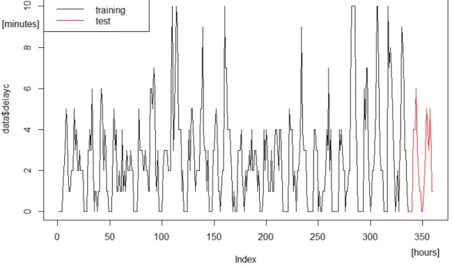
During one working day up to 500 single departures are registered on every stop based on number of routes operating. In order to determine the forecasts, the averaged values were assumed, calculated with one-hour accuracy (separately for every day of the week). These forecasts was taken as reference values for further analyses.

Fig. 1. Average delay values for selected stop (training and test sets) Source: own work.

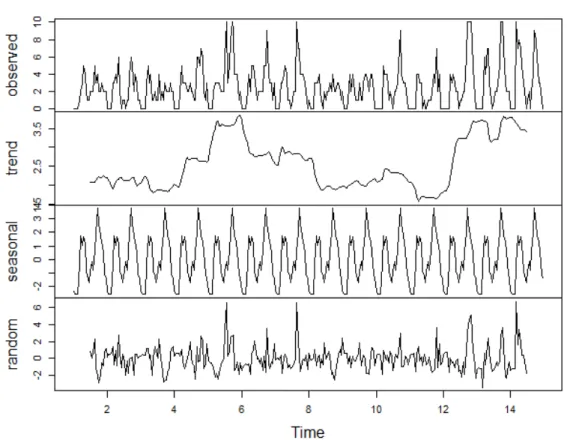
In Figure 1 the time series for average delay values for selected example stop in analyzed period of time was presented. Figure 2 illustrates the decomposition of time series classified and described with an additive model, with distinguished parts of trend, seasonal and random components.

Logistyka 4/2014

2700

Fig. 2. The decomposition of time series for average values of delays for selected stop Source: own work.

Fitting the one-dimensional time series was implemented using the auto.arima() function from forecast package. The summary of running procedure was given below:

> summary(arimamodel) Series: ttc

ARIMA(1,0,1)(2,0,2)[24] with zero mean Coefficients:

ar1 ma1 sar1 sar2 sma1 sma2 0.6054 -0.2027 0.2124 0.8259 0.0336 -0.7890 s.e. 0.0941 0.1155 0.0439 0.0448 0.0543 0.0533 sigma^2 estimated as 2.376: log likelihood=-622.13 AIC=1258.83 AICc=1259.17 BIC=1285.55

Training set error measures:

ME RMSE MAE MPE MAPE MASE Training set 0.03596753 1.424499 0.8908244 NaN Inf 0.4861297

Logistyka 4/2014

Fig. 3. The autocorrelation function for the residuals process of determined time series Source: own work.

Based on the plot of autocorrelation function it can be read, that most of the seasonal components has been identified correctly and included by the fitting procedure. The statistic value of Ljung-Box test is 21.26, while p value is 0.62, thus for the 24 period horizon there is a minor probability that the determined process is not a series of independent random variables and model presented in the example could be a subject for further optimizations.

> Box.test(forecast_arima$residuals, lag=24, type="Ljung-Box") Box-Ljung test

data: forecast_arima$residuals

X-squared = 21.2632, df = 24, p-value = 0.6232

Logistyka 4/2014

2702

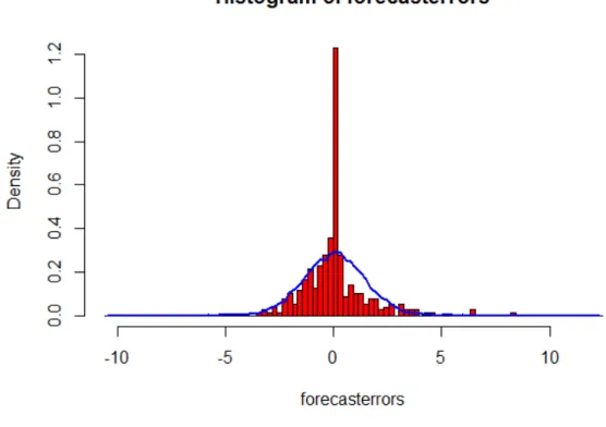
Fig. 4. The histogram with residuals for determined process Source: own work.

As a comparison to average delays calculated on the training set in the earlier stages, also two other forecasts have been determined:

− seasonal naïve method (equivalent to the process ARIMA(0,0,0)(0,10)[24]),

− exponential smoothing (STL + ETS(A,N,N)).

> accuracy(unclass(snaivemodel$mean), datasubsettest$delayc) ME RMSE MAE MPE MAPE

Test set -1.125 2.245366 1.541667 -Inf Inf

> accuracy(unclass(forecast_ets$mean), datasubsettest$delayc) ME RMSE MAE MPE MAPE

Test set -0.1460692 1.361311 0.9535684 NaN Inf

> accuracy(unclass(forecast_arima$mean), datasubsettest$delayc) ME RMSE MAE MPE MAPE

Test set -1.046412 1.643189 1.187099 NaN Inf

Logistyka 4/2014

Fig. 5. The comparison of forecasts developed using different prognostic models. Source: own work.

The forecast values obtained with an automatic script were evaluated using the accuracy() function of statistical package R. The forecasts developed by different prognostic model were compared with the vector of original real delays registered in the analyzed time period which was part of the training set for time series. The summary is given below:

> accuracy(results$prediction_avg, results$departure_delayed) ME RMSE MAE MPE MAPE Test set 0.7969148 4.316652 2.602414 0.09529932 0.3358216 > accuracy(results$forecast_snaive, results$departure_delayed) ME RMSE MAE MPE MAPE Test set 0.4104628 4.495918 2.764588 -0.01769953 0.3628042 > accuracy(results$forecast_ets, results$departure_delayed) ME RMSE MAE MPE MAPE Test set 0.8636643 4.339633 2.69881 0.09594112 0.3531142 > accuracy(results$forecast_arima, results$departure_delayed) ME RMSE MAE MPE MAPE Test set -0.3373395 4.323084 2.861028 -0.07843339 0.3739382

According to the values of ME, RMSE, MPE and MAPE errors it can be said, that the solution implementing the automatic model fitting using the one-dimensional ARIMA process gives satisfactory results, comparable to the model where only average mean value is taken as parameter.

Logistyka 4/2014

2704

Conclusions

The result of running the module is a generated forecast of transportation system state for the moment of defining the query by the end user, based on available historical data. Analogously to the example procedure presented for one stop discussed earlier, the forecasts are generated for all serviced stops, using the statistical package R. The further works include improvement of forecast values and optimization of model’s parameters.

Abstract

The presented article discusses the forecasting model of the tasks’ execution in the public transport system using the time series theory. The consecutive steps of building a model using the statistical package R has been described. Practical verification of the model was performed using real data acquired from the carrier performing services in public transport. The results obtained were rated positively, however, the need for further work on improving the quality of appointed forecasts has been stated.

Model prognostyczny realizacji zada

_ń

w systemie transportu

publicznego

Streszczenie

W przedstawionym artykule omówiono model prognozowania realizacji zadań w systemie transportu publicznego wykorzystujący teorię szeregów czasowych. Opisano poszczególne kroki budowy modelu przy wykorzystaniu pakietu statystycznego R. Praktyczną weryfikację modelu przeprowadzono z wykorzystaniem danych rzeczywistych pozyskanych od przewoźnika realizującego przewozy w transporcie miejskim. Uzyskane wyniki oceniono pozytywnie, zwrócono jednakże uwagę na konieczność dalszych prac nad poprawą jakości wyznaczanych prognoz.

Literature

[1] Bojda K.: Selected issues of timetable modelling for information systems purposes. (in:) Contemporary transportation systems: selected theoretical and practical problems: modelling of change in transportation subsystems. Gliwice 2011, p. 163-169.

[2] Brockwell P., Davis R.: Introduction to Time Series and Forecasting, Springer, New York 2002.

[3] Pyrga E., Schulz F., Wagner D., Zaroliagis C.: Efficient Models for Timetable Information in Public Transportation Systems. ACM Journal of Experimental Algorithmics 12/2008, p. 1-39.