Reconstructing Historic Glacier States Based on Terrestrial Oblique
Photographs
Samuel Wiesmann, Ladina Steiner, Milo Pozzi, Claudio Bozzini, Andreas Bauder, Lorenz Hurni
ABSTRACT: Fluctuations of glaciers result from climate variations. Understanding past glacier fluctuations is crucial when forecasting future glacier evolution. Observations of the frontal position have been carried out systematically in the Swiss Alps and worldwide since the end of the 19th century. The approach presented here aims to merge all available sources of information on frontal positions into one consistent, georeferenced database. All available original field data of Rhonegletscher is reworked and historic photographs are georeferenced using the monoplotting technique to complete and control the dataset. More than 100 states could be collected. The results are presented not only in a map, but also in an interactive oblique image.
KEYWORDS: Glacier, reconstruction, monoplotting, length change records, oblique view, 3-dimensional mapping.
Introduction
The measurement and documentation of length fluctuations of glaciers have a long tradition and are carried out annually on many glaciers in Switzerland (Glaciological reports, 1881-2011). Due to the relatively simple nature of this measurement, long data series have been collected. However, usually only measurements to local reference points were reported and no georeferenced coordinates exist. Many records cover inhomogeneities caused by the dislocation of such reference points, interruptions in long-term measurement campaign, changes in applied measurement method, or changing personnel. As a result, cumulative length change over longer periods therefore tends to show large discrepancies to known front positions from existing landmarks or documented states on maps or photographs.
Important information about glacier states is stored in terrestrial images, which can be found in good quality even from the second half of 19th century. Such images can be used to check or validate length change records. However, the use of historical pictures for accurate analysis of fluctuations of the glacier tongue or validating existing records requires georeferencing. In the presented study the monoplotting technique was applied to systematically evaluate available pictures and merge with maps and documented field data.
Data and study site
Rhonegletscher (46°36´ N, 8°23´ E) is a valley glacier located in the central Swiss Alps. In 2012, it covers an area of about 16 km2 with an elevation range from 2200 to 3600 m a.s.l. As most of the glaciers in the Alps and elsewhere, Rhonegletscher has retreated significantly since the middle of 19th
The tongue of Rhonegletscher is in close vicinity of the road over the mountain pass of Furka allowing a relatively easy access to many people. Already in the 15
century (Glaciological reports, 1881-2011). For the study presented here, all different available sources of information on documented frontal positions of Rhonegletscher are collected.
th
century intense trade and traffic over the pass is documented (Stadler, 2006). Combined with a good sight from the road onto the glacier and the spectacular icefall at Hotel Belvédère in particular, the area became a tourist attraction already in the early 19th century. Therefore, a large number of old terrestrial photographs and paintings exist, which document the tongue of Rhonegletscher or parts of it (e.g. Dumoulin et al., 2010). Figure 1a shows such a picture, which documents the glacier state of the year 1898.
Figure 1: Different sources for historic glacier states: Historic photograph (1a), field measurement report (1b), special map from field campaign (1c), and official Swiss national map (1d).
Starting in 1874, an extensive and long-term monitoring program was initiated (Mercanton, 1916). The data collected over the years is recorded in field reports and special maps (Figure 1b & 1c).
A unique and reliable source are the topographic maps of the official Swiss national map series. Published for the first time in the 1930s in scale 1:50 000 (Figure 1d) they were regularly updated. Starting in the 1950s, smaller and larger scales completed the map collection. These historic maps store important information of the past in general. Regarding glaciers, not only the glacier extent, but also the shape of the glacier surface with elevation information can be reconstructed (e.g. Bauder et al., 2007). In connection with the production of the map series, aerial images were acquired by the Federal Office of Topography swisstopo. The first available aerial orthophotograph of Rhonegletscher is from 1959, followed by newer images in irregular intervals of a few years until today. In addition, high resolved aerial images of the glacier tongue are acquired annually since 1968 due to ongoing efforts of glacier monitoring.
Methods
In order to achieve one consistent database of georeferenced information about the development of the frontal position of Rhonegletscher over the years, several methods are deployed, depending on the type of input data source.
Monoplotting principle for georeferencing historic photographs
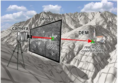
Single images can be georeferenced, under certain conditions, using the monoplotting principle (e.g. Konecny, 2003, Rady, 1984). Beside the oblique image, the following data is required to complete georeferencing successfully: a georeferenced map or orthophotograph, a digital elevation model (DEM), control points with known coordinates, and the camera parameters. However, oblique photographs are usually neither georeferenced nor do they have known geographical or optical camera parameters, such as camera position, viewing direction, image center, or focal length. The unknown camera parameters can be approximated using an iterative camera calibration algorithm, though. The goal is to place the image and the camera in world space, so that a ray from the camera intersects both, a point on the image as well as the DEM at the corresponding real point (Figure 2). Such corresponding control points must be visible in the oblique image and on the orthophotograph. Several pairs of control points enable the calibration and the reconstruction of the camera parameters, particularly, the camera position and orientation.
Once the camera is successfully calibrated, oblique image and orthophotograph are bidirectionally linked in a way, that each image pixel has its corresponding pixel on the orthophotograph and on the map respectively: the oblique image is georeferenced. This allows digitizing, e.g. the position of the glacier tongue, directly in the oblique image, whereby the digitized polyline is stored in real world coordinates synchronously. Several
images from different years allow for a collection of glacier states, which can be stored in one spatial database.
Figure 2: Schematic representation of the system elements of monoplotting: Camera, oblique photograph, DEM, and the real world (Bozzini et al., 2011)
Only a few software solutions have been developed for georeferencing terrestrial, single images on the basis of the monoplotting technique, e.g. OP-XFORM (Doytsher and Hall, 1995), the Georeferencing oblique terrestrial photography (Corripio, 2004), and others. However, this software is very technical and only usable for specialists.
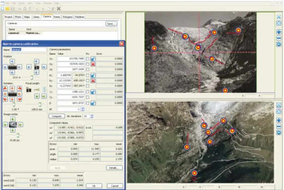
The lack of user-friendly and intuitive software on the one side, and the increasing general interest of using historic images for studies on the other side (e.g. Roush et al., 2007, Kull, 2005), is the reason why the “WSL monoplotting tool” is being developed since 2009 (Bozzini et al., 2011). This software makes use of the principle described above and further insight is given in the results section below. Figure 3 shows the user interface of the software after a successful georeferencing of a historic photograph. The oblique image and the aerial orthophotograph are linked and drawing an object in one of the pictures simultaneously displays this object in the other. The yellow-red circles symbolize control points used for georeferencing.
Figure 3: User interface of the WSL monoplotting tool: successfully georeferenced historic oblique photograph (top right) and respective, linked orthophotograph (bottom right).
Frontal positions from field reports and maps
The reports and maps from the field campaigns (Figure 1b and 1c) are drawn on paper. Some of them are published (e.g. Mercanton, 1916), other originals are available from the archives of the glaciological commission (SANW, 2001). All of them have been scanned and georeferenced for this study. All documents provide information, which allows georeferencing in one way or another. Some of them contain reference points in the projected coordinate system that is still in use in Switzerland today. Some of the older maps were based on a slightly different definition of the reference system that had to be transferred.
Most unpublished field reports contain local reference points, which have no georeferenced coordinates, and were used as local reference for the measurements for many years. Based on other field notes, it was possible to project the local reference points on a georeferenced map, what enabled the georeferencing of these field reports. The historic maps from the Swiss national map series are provided by the Federal Office of Topography (swisstopo) directly as georeferenced raster images.
For this study, all the georeferenced data is transformed, if necessary, and kept in only one current reference system (CH1903-LV03). Once these maps and field reports are georeferenced, the glacier boundary is digitized manually and stored in the same spatial database as the states derived from the historic photographs.
Reanalysis of glacier length change records
All glacier states stored in one consistent spatial database provide an overview of the glacier length fluctuations. A systematic re-interpretation of these fluctuations along a central longitudinal profile is achieved. For the individual states between 1879 and 2010, this re-interpretation is compared to the published length change results in the Glaciological reports (1881-2011). In years where oblique photographs and other reliable data about the position are available, the accuracy was evaluated.
Results
Accuracy analysis of the monoplotting results
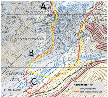
In some years, the frontal position is available from different sources. This allows for a direct comparison of the results in order to assess the reliability of the different methods. In the following, the results of the comparison for the years 1874 and 1929 are discussed. For both years, oblique photographs in good resolution as well as accurate maps are available (these photographs are shown in Figure 11 in low resolution). Figure 4 and 5 show the frontal position reconstructed from maps in red, and reconstructed from historic photographs in yellow.
The photograph from 1874 does not cover the glacier terminus (marked with a C in Figure 4). In the area visible on the photograph, the two lines have an average distance of 12.6 meters.
Two reasons can be imagined where the differences in area A (up to 70m) could originate from. The first is the “flat angle problem”: in this area, the angle of incidence of the ray of the camera with the DEM is small. A small shift in the image space leads to a large error in real world space. This is one of the standard problems that can occur when applying the monoplotting principle. The second reason could be more operator-dependent: the glacier is heavily debris-covered in this area, what makes the definition of the glacier boundary ambiguous.
The diverging results in area B could be explained with a “hidden area”. The real glacier boundary is not visible from the camera position, because it is hidden by parts of the glacier (and DEM respectively), which are closer to the camera position. This is a second standard error source of the monoplotting technique.
Figure 4: Frontal position in the year 1874 from different sources. Yellow line obtained by evaluating a historical photograph, red line by georeferencing and digitizing a special map from field campaign.
Basemap from 1999.
The average distance between the resulting frontal positions for the year 1929 (Figure 5) is 12.5m. Largest differences (D, E, both up to 40m) occur in areas with very high slope values. The underlying DEM may be inaccurate and cause errors.
Figure 5: Frontal position in the year 1929 from different sources. Yellow line obtained by evaluating a historical photograph, red line by georeferencing and digitizing a map. Basemap from 1999.
C
A
B
D
For the year 2010, the data available allowed a calibration of the camera with an oblique photograph, an orthophotograph, and a DEM from exactly the same day. In particular, this facilitates the setting of control points, because control points can easily be identified in both pictures and can also be set on the glacier surface. Furthermore, the DEM represents exactly the shape visible on the photo. These specific circumstances support a good calibration of the camera and the average distance between the resulting positions could be reduced to 3.6m.
Tests showed that the camera calibration can be improved, if the accurate position of considered control points is known from field survey. However, it was not possible to compare the resulting frontal positions in this case, because the border of the glacier is not clearly visible on the used photographs.
Reanalysis of glacier length change records
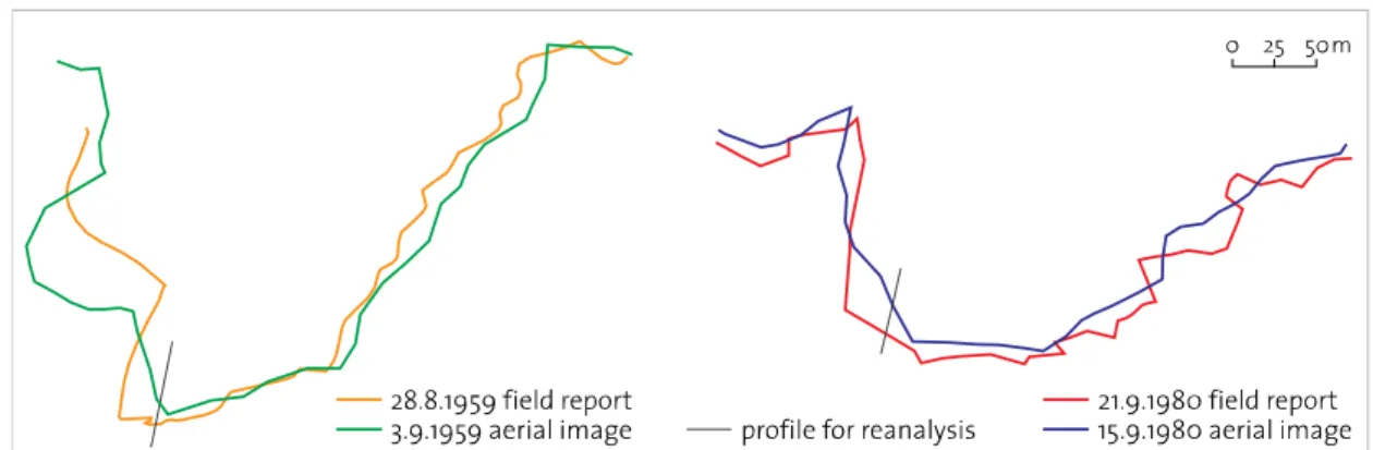
For the years 1959 and 1980, the frontal position could be derived from two different and independent sources and independent from the monoplotting technique. In both years, digitized positions from original field reports and a photogrammetrical analysis of aerial orthophotographs are available for comparison (Figure 6). They have been recorded with about one week time lag, what could explain a small part of the deviations. However, the overall shape fits quite well, even though they differ on both sides to some extent. In the year 1959, the average distance between the two lines is 11.2m and 7.8m for the year 1980.
Figure 6: Comparison of frontal position derived from field reports and from aerial images for 1959 (left) and 1980 (right).
A total of 104 georeferenced frontal positions have been collected so far, which cover the time period from 1602 until 2010. For the first time, they are available in one homogenous dataset. This enables an interpretation of the length fluctuation over more than 400 years. The analysis of glacier length change is conducted along one central
longitudinal profile. This profile and a selection of glacier outlines are displayed in Figure 7. During the entire time period, Rhonegletscher retreated about 2600m.
Figure 7: Selected historic glacier states of Rhonegletscher between 1602 and 2010 and central profile (red) used for reanalysis of length change.
For the time period from 1879 until 2010 (131 years), the reanalyzed length changes are compared to the published values in the Glaciological reports (1881-2011). The cumulative length change of 1539m deviates by 273m from the values reported so far (Figure 8). The evolution of differences between the two cumulative length changes can be roughly divided into two periods with different trends: 1879 until 1910 and 1910 until 2010 (green graph in Figure 7). Most of the deviation accumulates in the first period. During the second period, the curves fit very well: the mean difference in this second part is only 0.8m.
Figure 8: Cumulative length change based on glacier database as published in glaciological reports (blue) and after reanalysis (red) for the period 1879 until 2010; Difference between these two length changes
(green).
Visualization
Beside standard visualization of the resulting frontal positions on a static 2D map as shown for example in Figure 7, selected glacier states are also visualized on the georeferenced oblique images. It is expected that this makes interpretation more intuitive, especially for non-experts, because results are shown in a familiar view of the environment. One Example is shown in Figure 9.
Figure 9: Oblique view on Rhonegletscher visualizing selected glacier states between 1874 and 2010 (Pozzi, 2012; Photographer: Geiger, 1962).
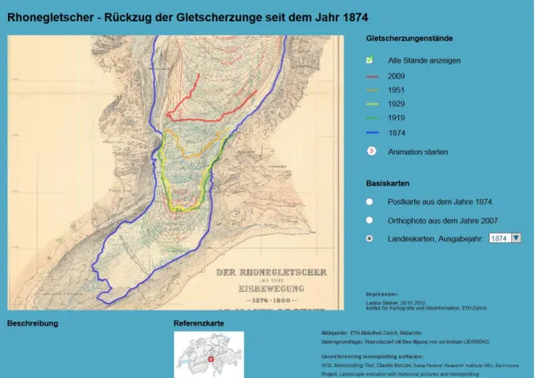
A web-based prototype was also developed, using a subset of the glacier states (Steiner, 2012). It combines the interactive visualization on a 2D map and on an oblique photograph of the glacier. The user can switch between the 2D mode (Figure 10) and the oblique view mode (Figure 11) by clicking a radio button. Several maps and aerial orthophotographs are available for background visualization in 2D.
By clicking on one of the visualized frontal positions, additional meta-information is available and the respective historic photograph is displayed in a separate window (Figure 11).
A revised version of the prototype with extended functionality is currently under development.
Figure 10: Prototype of interactive web-based visualization: 2D mode (Steiner, 2012).
Figure 11: Prototype of interactive web-based visualization: oblique view mode with a photograph from 1874 in the main window and one from 1929 in the pop-up window (Steiner, 2012).
Conclusions
A substantial amount of terrestrial images can be found in good quality even from the second half of 19th
This study aims to merge all available sources of information on frontal positions into one consistent, georeferenced database. The data series available now covers a time period of more than 400 years. It reaches further back in time and contains 104 georeferenced glacier states. The cumulative length change for the period since 1879 deviates about 270m (20%) from the values used so far. The sources and methods presented here deliver reliable results, what is shown for several selected years.
century. Using the WSL monoplotting tool, such images can easily be georeferenced and evaluated. The accuracy achieved is good enough for many fields of application. From the glaciological perspective, glacier states can be reconstructed e.g. for long ranging time series.
The available database allows the visualization in one map or in an interactive, web-based tool. This encourages specialists, glaciologists in this case, to present their results of investigations to the public, what may support the dialog between public and experts.
References
Bauder, A. Funk, M. and Huss, M. (2007) Ice-volume changes of selected glaciers in the Swiss Alps since the end of the 19th century. Annals of Glaciology. 46, pp. 145-149.
Bozzini, C. Conedera, M. and Krebs, P. (2011) Ein neues Tool zur Georeferenzierung und Interpretation von terrestrischen Schrägbildern. e-geo.ch Newsletter. 27, pp. 16-17.
Corripio, J.G. (2004) Snow albedo estimation using terrestrial photography. International
Journal of Remote Sensing, 25, 24, pp. 5705-5729.
Doytsher, Y. and Hall, J.K. (1995) Fortran programs for coordinate resection using an oblique photograph and high-resolution DTM. Computers & Geosciences
Dumoulin, H. Zryd, A. and Crispini, N. (2010) Glaciers – Passé-présent du Rhône au
Mont-Blanc. Éditions Slatkine.
, 21, 7, pp. 895-905.
Glaciological reports (1881-2011) The Swiss Glaciers, Yearbooks of the Cryospheric Commission of the Swiss Academy of Sciences (SCNAT), No. 1-128, (http://glaciology.ethz.ch/swiss-glaciers/).
Konecny, G. (2003) Geoinformation: Remote Sensing, Photogrammetry and
Kull, C.A. (2005) Historical landscape repeat photography as a tool for land use change research. Norwegian Journal of Geography
Mercanton, P.L. (1916) Vermessungen am Rhonegletscher 1874-1915. Neue Denkschriften der Schweizerischen Naturforschenden Gesellschaft, Vol 52.
, 59, pp. 253-268.
Pozzi, M. (2012) Rekonstruktion von Gletscherzungenständen aus terrestrischen Bildern
und Sammlung der historischen Längenänderung am Rhonegletscher. Bachelor
thesis, Institute of Cartography and Geoinformation ETH Zürich.
Rady, J. (1984) Die dritte Dimension aus einem Einzelbild. Mitteilungen Blaue Reihe, Nr 36, Institute of Geodesy and Photogrammetry IGP, ETH Zurich.
Roush, W. Munroe, J.S. and Fagre, D.B. (2007) Development of a spatial analysis method using ground-based repeat photography to detect changes in the alpine treeline ecotone, Glacier National Park, Montana, U.S.A. Arctic, Antarctic and Alpine Research
SANW (2001) Archiv der Glaziologischen Kommission der SANW. Verzeichnis der Geschäftsakten, Berichte, Pläne usw. des Gletscherkollegiums und der Gletscherkommission von 1870 bis ca. 1955 (Rechnung bis 1963, Protokolle bis 1984) Glaziologische Kommission der SANW. ETH-Bibliothek, http://dx.doi.org/10.3929/ethz-a-004190495, last visited 8/13/2012.
, 39, 2, pp. 297-308.
Stadler, H. (2006) Furkapass. In: Historisches Lexikon der Schweiz (HLS), Band 5, pp. 29-30. Basel: Schwabe Verlag.
Steiner, L. (2012) Reconstruction of glacier states from geo-referenced, historical
postcards. Master thesis, Institute of Cartography and Geoinformation ETH
Zürich.
Image sources: Fig. 1a and images included in Fig. 3 and Fig. 11: Bildarchiv ETH-Bibliothek Zürich, http://ba.e-pics.ethz.ch. Fig. 1d and basemap in Fig. 4, Fig. 5, and Fig. 7: reproduced with the authorisation of swisstopo (JA100120), Bundesamt für Landestopografie swisstopo (Art. 30 GeoIV): 5704 000 000.
Samuel Wiesmann, dipl. geogr., Institute of Cartography and Geoinformation,
Wolfgang-Pauli-Strasse 15, ETH Zurich, 8093 Zurich, Switzerland. Email <swiesmann@ethz.ch> Lorenz Hurni, Professor, Institute of Cartography and Geoinformation,
Wolfgang-Pauli-Strasse 15, ETH Zurich, 8093 Zurich, Switzerland. Email <lhurni@ethz.ch>
Andreas Bauder, Dr. sc. nat., Laboratory of Hydraulics, Hydrology and Glaciology (VAW),
Gloriastrasse 37/39, ETH Zurich, 8092 Zurich, Switzerland. Email <bauder@vaw.baug.ethz.ch>
Claudio Bozzini, Dipl. Math. ETH, Swiss Federal Institute for Forest, Snow and Landscape
Research WSL, Via Belsoggiorno 22, 6500 Bellinzona, Switzerland. Email <claudio.bozzini@wsl.ch>