Benchmarking of Classical and Machine-Learning Algorithms (with special emphasis on Bagging and Boosting Approaches) for Time Series Forecasting

(1)

Master Thesis in Statistics

at Ludwig-Maximilians-Universität München Faculty for Mathematics, Informatics and Statistics

Department Statistics

Benchmarking of Classical and Machine-Learning Algorithms

(with special emphasis on Bagging and Boosting Approaches) for

Time Series Forecasting

presented by Uwe Pritzsche

Advisor: Prof. Dr. Christian Heumann

Examiner: Prof. Dr. Christian Heumann

(2)

(3)

Abstract

The goal of this Master thesis is to evaluate the time series forecast capability of several Machine Learning approaches, in detail Neural Nets, Random Forests, Kernel Machines (Support Vector Machines and Gaussian Processes), tree-based and component-wise linear and spline-based Boosting, by a comparison with classical ARIMA and ETS models. For the classical models also time-series specific bagging approaches, Moving Block Bootstrap and Maximum Entropy Bootstrap, are tested. For this purpose, extensive benchmarks are conducted, utilizing the well-known official

Tourism, M3 and NN5 competition data with the latter comprising also several exogenous covariate effects. In order to uncover specific problems the Machine Learning approaches reveal for the typical time series components of trend and seasonality, a simulation is executed helping in understanding some benchmark results as well as suggesting combinations of the Machine Learning algorithms with classical deseasoning and detrending steps (Box-Cox transformation, STL decomposition, seasonal Differencing). Furthermore different multi-step-ahead forecasting strategies are applied to the NN5 time series.

It can be shown that ARIMA based models are competitive to Machine Learning models for the investigated classical (without any exogenous covariates) time series forecasting situation. On the other hand, ETS approaches are less promising. And the classical models can be enhanced by the tested bagging approaches with the easy-to-use Maximum Entropy Bootstrap showing some advantages over the more known Moving Block Bootstrap. One simple but very important result from the conducted simulation using phenotypic time series is represented by the fact that tree-based models as well as splines with a locality property are incapable of modeling a future trend. In such situations these approaches must be combined with a detrending step resulting in inferior results also for the tree-based boosting model (gbm) as one of the most popular Machine Learning algorithm. Actually the Support Vector Machine is the most promising candidate mostly outperforming all other methods including classical approaches, especially in conjunction with exogenous covariates. Even though Gaussian Processes can be founded in the same theoretical context of Kernel machines, this approach is demystified by its results. Further enhancing the Machine Learning models by direct and hybrid (combination of recursive and direct) forecasting strategies does not reveal any substantial improvements for the tested NN5 series. Interestingly, the benchmark on the M3 data conducted in this thesis seem to be the first one revealing a more than competitive prediction of special naïve methods for most series making performance conclusions of other studies based on this data highly questionable.

(4)

(5)

1 Introduction

1.1 Motivation

Time Series Forecasting has a long history not only in scientific field but in practice as well. Beside the most known usage for stock market forecasting numerous additional applications in business exist, like Budget Forecasting, Inventory Planning and Energy Consumption Prediction, to mention just a few. And in the ages of big data and the internet of things more and more fine grained information is recorded not only with respect to the timely development of interested target leading to new applications in many fields. Additionally to the chronological target variable more exogenous information is available increasing the set of possible covariates. This evolution brings into play relatively new (compared to the classical methods) algorithms from the Machine Learning field which have proven a remarkable performance in classical prediction problems (without time related information) often outperforming classical statistical models like linear regression for instance. But it is also of interest whether these modern approaches can also compete in a classical time series setting using just the consecutive target variable information to predict the future. In fact this ability seems to be a prerequisite to at least improve forecasting results settings with high exogenous covariate influence.

The most used Machine Learning model in the time series context so far are Neural Nets (referred to

as nnet in this thesis). But especially tree based algorithms in conjunction with bagging, i.e. Random

Forests (rf), and boosting (gbm) are very popular in the Machine Learning community due to some

properties highly advantageous for prediction like automatic interaction detection or robustness against irrelevant predictors. The latter holds also for boosting approaches in conjunction with linear (glmboost) or semi-parametric (gamboost) regression models which further have much better interpretability capabilities as well and are therefore favored in the statistical community. All these models account for the correlation of the target variable values by using lagged target information. An alternative that recently got very popular in the Machine Learning community are Gaussian Processes

(gp) which are based in the theory of so-called Kernel machines as the covariance matrix of the target

can be interpreted as a Kernel matrix. The ancestor of a such Kernel machines are the well-known

Support Vector Machines (svm) which originated in classification task but can be adapted for

regression problems as well.

Especially the success of Random Forests creates attention for bagging (bootstrap aggregation) as a general tool for improving forecasts. If, as common for the Machine Learning models, the lagged target variable information is just added to the standard covariate set, the bootstrapping can be conducted as usual, i.e. random sampling with replacement. But it the modeling approach like for the classical Arima (or for Gaussian Processes as well!) needs the original data order for estimating the model the usual approach is not applicable as it destroys this order. Therefore special sampling schemes must be applied. One part of this thesis work tests the improvements which can be gained for classical models by bagging with the well-known Moving Block Bootstrap as well as a more modern and easy-to-use approach, the Maximum Entropy Bootstrap.

All in all the aim of this thesis is to shed some light onto the performance of all above mentioned machine learning approaches compared to classical models and bagging approaches for the latter. This is done by benchmarking the methods utilizing several data sets from known official competitions,

i.e. the well-known classical M3 (Makridakis & Hibon (2000)), the Tourism competitions

(Athanasopoulos et al. (2011)) and the NN5 contest (Crone (2009b)) comprising additional exogenous

(8)

1 Introduction

Time series forecasting exhibit some special characteristics not common in the usual prediction setting like a whole bunch of official metrics for measuring performance that are highly sensitive to the forecasts. Moreover one is usually interested in multi-horizon forecasts, i.e. predictions not only for the next future time point but e.g. for the next few seasons raising the question whether to reuse forecasts as inputs in so-called recursive forecasts or better use direct predictions employing just known information. This also complicates the assessment of forecast accuracy as the performance can differ from horizon to horizon further depending on the evaluation metric used. Consequently some attention is put on the careful handling of performance evaluation in this thesis.

Also somewhat uncommon for the Machine Learning models are the usual time series components of trend and seasonality. At first sight the trend component does not seem to represent a problem for prediction models but one has to keep in mind that the trend has to be put forth into the future and therefore outside the range of the time input variable, resulting in critical modeling problems, especially for tree based approaches for instance. Related problems might grow when dealing with increasing seasonality. In order to uncover such general problems Machine Learning models might have with these components, a simulation study is conducted that reveals some interesting insights that not only help in understanding benchmark results but also suggest different variants of each Machine Learning model.

Actually the typical approach with Machine Learning models for handling the seasonality is using seasonal dummy variables. Alternatively it is possible to combine the Machine Learning algorithm with classical means for stripping of the seasonality like seasonal differencing, a modeling approach invented in classical ARIMA modeling, or decompositions like STL (seasonal-trend decomposition based on Loess). Also initial Box-Cox transformation of the time series might help in case of increased seasonality for instance. It is of interest whether the Machine Learning approaches can profit from such combined approaches which is therefore extensively tested by applying several variants of each algorithm.

In order to assess the performance of these combination approaches they must be compared to the corresponding classical models, at least with the most popular representative, i.e. ARIMA models. Usually this model class is embedded in a whole modeling operating manual, the Box-Jenkins approach. On the other hand, ETS (exponential smoothing) models are mostly neglected by the academic canon even though successfully applied by practitioners for a long time. A reason for this disregard might be a lack of statistical founding of this initially heuristic approach just recently patched by Hyndman et al. (2008) utilizing state space modeling. This thesis also tries to avoid the common lack of dedication for this (in non-academic community well-known) modeling approach.

Last but not least the extensive evaluations conducted in this theses are motivated by several other studies (listed in the following Chapter 1.2) that lack of several before mentioned aspects. For instance, usually only a few of before mentioned Machine Learning approaches are tested. Or no comparison with classical methods is conducted. More severe in this conjunction is the typical practice of neglecting to conduct at least one naïve forecast or several naïve forecast variants as benchmarks in order to assess the forecastability of the series which is crucial especially for the M3 competition data as will be shown later. Sometimes the investigated time series are too short or too few in number which prevents from getting a valid result which is also the problem when just 1-step-ahead forecasts are executed. In case of multi-horizon forecasts nearly always only the recursive strategy is applied. Some studies are more theoretically motivated and therefore lack of real-life datasets comprising trend and seasonality. Last but not least just a few authors try different deseasonalizing strategies.

This thesis is structured as follows: Already in this introductory chapter the related work is discussed. Then Chapter 2 first explains the benchmark datasets with a more detailed discussion of possible covariate effects for the NN5 time series. Further prerequisites for the investigations like forecasting strategies as well as the applied evaluation approach follow, already producing important insights. The

(9)

1.2 Related Work

classical models are explained in detail in Chapter 3 together with the possible general preprocessing steps, i.e. Box-Cox transformations and STL decomposition. All explanations are accompanied by some initial benchmark results. This holds also for the passage dealing with the utilized bagging approaches for the classical models before presenting a comparison of just the classical models for all three competition benchmark series at the end of this Chapter. The theory of the Machine Learning algorithms is explained in Chapter 4. In order to get a direct impression of the performance of these models some benchmark insights are added even though this kind of anticipates some results of the simulation study presented at the end of Chapter 4 using some phenotypic time series to uncover general problems of the Machine Learning approaches with time series (more precise the trend and seasonal component). Chapter 5 is dedicated to the overall benchmark results comparing all classical and Machine Learning approaches for all competition benchmark data. The thesis closes with a summary giving also a short outlook.

1.2 Related Work

Literature for applying Machine Learning or Data Mining approaches for time series forecasting is relatively sparse. Reasons for, but also opportunities resulting from this gap, are shortly discussed in Crone (2009a), listing what forecasters can learn from Data Mining and vice versa. Also Gooijer & Hyndman (2006) in their overview article “25 years of time series forecasting” spend their attention regarding machine learning techniques just on neural nets in the chapter about nonlinear methods.

Nonetheless they state that “with the ability of very large datasets and high powered computers, we

expect this [bagging and boosting approaches] to be an important area of research in the coming years”.

The following subsections first list related investigations for machine learning approaches in general and then dedicate two subsections explicitly for bagging techniques, comprising classical bootstrapping of time series, and boosting approaches.

Machine Learning approaches

The most used algorithms from Machine Learning field for forecasting so far are neural nets (nnet).

Already in the famous M3 competition the nnet is the only non-classical method used (Makridakis &

Hibon (2000)). Furthermore Krollner et al. (2010) nicely show in their overview article for financial time series forecasting that ANN is the dominant technique in this area (mostly used for 1-day ahead forecasting).

Apart from ANNs the majority of investigations using Machine Learning models are restricted to

k-nearest neighbor (kNN), support vector machines (svm), gaussian processes (gp) and boosting

techniques with trees (gbm), component-wise linear (glmboost) or spline (gamboost) models.

For example, the relatively extended study of Ahmed et al. (2010) compares nnet, kNN, svm, gp and

CARTs (classification and regression trees) utilizing different preprocessing steps regarding detrending techniques (lagged target values, differencing and moving average filtering). Furthermore they deseasonalize in advance leaving just the remainder for the ML methods for forecasting and incorporate a tuning of the number of lagged target values. Unfortunately they apply these methods on the whole M3 competition putting all categories of time series into one pot (which is problematic as discussed in Chapter 2.3.2). Also only 1-step ahead predictions are done and no comparison with a

naïve method or classical approaches is conducted. With these restrictions nnet and gp end up as the

(10)

1 Introduction

Much less models are used in Lora et al. (2004) who let kNN compete with dynamic regression models for a 24h energy load forecasting problem and show superior performance for the kNN approach.

For a similar problem in the GEFCom2012 forecasting competition (Hong (2012)), Lloyd (2014)

applies gp using “periodic” kernel in a decorrelated ensemble with gbm. Actually the gp performance

as standalone prediction was far behind the gbm. Interestingly no lag information was utilized apart

from an implicit usage by the gp correlation.

For this competition Hong et al. (2014) summarize the methodology of the top competitors, wondering why no classical ARIMA model is used by anyone. Basically most of the winning teams apply linear regression with splines, sometimes enhanced by boosting.

The second placed team of the NN5 competition (Crone (2009b)), Andrawis et al. (2011), utilize an

exhausting ensemble of several nnet and gp models with classical ARIMA and ETS approaches,

claiming a big advantage by their somewhat difficult desesonalizing preprocessing.

Again the nnet is chosen for a study of Matteo et al. (2013) for temperature forecasts in buildings

resulting in better prediction than using a classical standard regression models with and without autoregressive components.

Similarly Kandananond (2012) lets nnet and svm compete against classical ARIMA models but just for

6 really short datasets leaving svm as the winner.

Also the svm takes part in a comparison with nnet and ForecastPro, a commercial forecasting

package basically using an ARIMA-ETS combination, applied on simulated time series in Crone et al. (2009). Actually the simulation study of Chapter 4.5 in this thesis is influenced by their simulated combinations of no, additive or multiplicative seasonality with no, linear, progressive or degressive trend each combined with different noise levels. Also some lag selection tuning was conducted by

them utilizing the PACF (partial autocorrelation function). Here svm, followed by nnet, wins the

nonlinear, i.e. multiplicative seasonality and/or progressive or degressive trend case whereas for the

linear series the classical ARIMA-ETS combination outperforms svm and nnet.

A different intention has Bontempi et al. (2013), explaining different Machine Learning forecasting strategies, including recursive and direct forecasts, basically using a kNN model.

Related is the study of Taieb & Hyndman (2012a) using a combination of initial recursive autoregressive prediction and a direct adjustment for the forecast error by a kNN model. They apply their method to simulated series as well as to the M3 and NN3 benchmark datasets with mixed results regarding forecast performance. A more detailed presentation of the NN5 results together with additional averaging strategies can be found in Taieb et al. (2012c). For preprocessing they use the before mentioned deseasonalizing steps from Andrawis et al. (2011) for this data.

Taieb & Hyndman (2014) further apply a modification of their own approach described above by using

a direct gamboost (with bivariate interaction of covariates) based forecast on the residuals of a STL

decomposition followed by a recursively applied ARIMA model for the M3 and NN5 competition datasets. This builds the bridge (apart from above mentioned Lloyd (2014) and Hong et al. (2014) mentioned above) to the next subsection looking at boosting techniques applied to time series forecasting.

Boosting

For the GEFCom2012 competition Taieb & Hyndman (2012b) compete with a combination of recursive

and direct forecasts of gamboost models with intensive lag value usage finishing fifth out of 105

teams.

A very promising investigation can be found in Robinzonov et al. (2010) showing the results of a

(11)

1.2 Related Work

autoregressive function of nonlinear time series. Actually glmboost shows impressive performance in

identifying the data generating lags. But the study also states that “strong serial dependence might

mislead the fitting procedure [i.e. gamboost] to produce erroneous transformations”. A final

comparison of forecast performance for some macroeconomic time series favors the linear boosting approach.

These nonlinear simulations together with some simulated linear time series are already discussed in Shafik & Tutz (2007).

Furthermore Buchen & Wohlrabe (2011) try to apply glmboost based direct forecasts to some

macroeconomic time series ending up with mixed results regarding the performance.

Bootstrap

A good overview of classical bootstrap methods for time series, i.e. mainly Block, Sieve and Stationary bootstrap, is given in the more technical paper from Härdle et al. (2003) concentrating on the accuracy of the methods for parameter estimation of a sample. The more readable summary from Kreiss & Lahiri (2012) on the other hand focusses more on advantages of the different methods in different data situations. Even though the Stationary bootstrap (Politis & Romano 1994) has the appealing capability of preserving the stationarity property, its success seem to be limited as “with respect to higher order properties the moving block bootstrap outperforms the version with non-overlapping blocks and both achieve a higher order accuracy as the stationary bootstrap” (Mammen & Nandi (2012)).

The more recent approach of Maximum Entropy Bootstrap (MEboot) is invented in Vinod & Lopez-de-Lacalle (2009) and concentrating on showing the main advantage of this approach, nicely summarized by the author with “the algorithm's practical appeal is that it avoids all structural change and unit root type testing involving complicated asymptotics and all shape-destroying transformations like detrending or differencing to achieve stationarity”. Furthermore the authors state that “the constructed ensemble elements retain the basic shape and time dependence structure of the autocorrelation function (ACF) and the partial autocorrelation function (PACF) of the original time series.”

Above resources concentrate more on the statistical properties of the different drawing techniques. Applications of bootstrap methods for time series forecasting by bagging the predictions of the different samples can be found e.g in Fan & Hyndman (2010) who use block bootstrap samples to get a complete distribution of prediction intervals when applying generalized additive models.

Bergmeir et al. (2014) improve the accuracy of forecasts by a moving block bootstrap applied on the remainder of a STL decomposition of M3 competition data and forecast with an ETS model. This is one of the rare studies also assessing the lift of initial Box-Cox transformations of the target variable. Cordeiro & Neves (2009) utilize the ETS initially followed by an ARIMA on the residuals before ending up in bootstrapping the residuals left over from this process. This parametric bootstrap approach, similar to the so-called SIEVE bootstrap, shows mixed behavior when applied on the M3 competition data.

Contrary to the typical bagging approach for Machine Learning methods (i. e. bootstrap as usual with lagged target information as standard covariates) Kourentzes et al. (2014) use a combination of classic bootstrap methods and ANN models by bagging with the moving block bootstrap to improve forecast accuracy, suggesting a median instead of a standard mean aggregation in the bagging step.

(12)

(13)

2 Prerequisites

2.1 Benchmark Datasets

For the forthcoming benchmarks the mostly used time series datasets utilized in other academic investigations are chosen. In detail these are the M3 competition datasets (Makridakis (2000)), the Tourism data from the Tourism2 competition hosted on Kaggle (Athanasopoulos et al. (2011)), and the series used in the NN5 competition (Crone (2009b)). Only the latter allows deriving additional exogenous effects like holiday, Christmas or Easter whereas the Tourism and M3 datasets are classical time series just comprising the consecutive target variable information. The latter holds as well for 300 simulated ARIMA series (see Chapter 3.1 for an introduction to Arima time series), named

Arimasim in the following. Regarding Tourism and M3 it was decided to use only the most fine-grained data, i.e. the monthly data. Furthermore only time series comprising more than 120 time points are used, ending up in removing one Tourism and several M3 series (see below).

Tourism

The monthly Tourism data comprises 365 time series (after removing 1 series having less or equal

120 time points). Figure 2.1shows the distribution of the number of time points. The maximum horizon

to forecast is 24. Unfortunately the data source from Kaggle website does not comprise the testing data, therefore the last 24 time points for each series are used instead for the test fold which is also the reason why a comparison with the official contest results can only be given on a qualitative level. Most of the series show a trend and seasonality (sometimes increasing); some typical examples are

plotted in the Appendix (see “A Supporting Plots and Tables”). In order to allow Box-Cox

transformations (cf. Chapter 3.3) a constant c=1 is added to have all series consisting of only strictly positive values.

The winning methods for this competition conducted in 2010 are presented in the International Journal of Forecasting (Brierly (2011b), Baker & Howard (2011)) but also described in short on two Kaggle blog posts (Brierly (2011a), Baker (2010)). Basically these solutions used a heuristic approach and an ensemble of classical (ETS and ARIMA, cf. Chapter 3) models respectively. Furthermore an extensive comparison of classical approaches applied on these data is available in Athanasopoulos et al. (2011), the accompanying paper for this competition. Main result for the monthly series is that ARIMA methodology is most accurate when considering MASE performance metric (see Chapter 2.3.1) and exhibits also clearly better predictions than a seasonal naïve forecast (cf. Chapter 2.3.2).

M3

The used monthly M3 data consists of 1010 series (after removing the shortest ones, see following

explanations) from 5 different areas named DEMOGRAPHIC, FINANCE, INDUSTRY, MACRO,

MICRO. The category OTHER is removed as all time series of this area has less or equal 120 time points which is the case for 418 time series in total. Figure 2.2 shows the distribution of time points for the remaining data sets. Some examples series are also plotted in the Appendix.

Results from this competition, with a maximum horizon to forecast of 18, are described in Makridakis & Hibon (2000) and several accompanying papers published in the same edition of the International

Journal of Forecasting. The main result, which is somewhat surprising at first sight, is that “simple

methods developed by practicing forecasters (…) [i.e. ETS] do as well, or in many cases better, than statistically sophisticated ones like ARIMA (…)”. Actually Chapter 3.2 of this thesis explains that ETS

(14)

2 Prerequisites

models can be put into a strict statistical frame and that many ETS model are also equal to ARIMA models.

It should already be mentioned that the usage of the M3 data for algorithm benchmarking is highly questionable as explained in Chapter 2.3.2. Despite this fact and the age of the competition datasets, these time series are still used in several investigations, e.g.: Cordeiro & Neves (2009), Ahmed et al. (2010), Taieb & Hyndman (2012a), Taieb et al. (2012c), Bergmeir et al. (2014), Taieb & Hyndman (2014).

NN5

This more recent competition from 2008 comprises 111 time series consisting of daily ATM withdrawal amounts in UK, each comprising 791 time points from 18/03/1996 – 17/05/1998 (i.e. > 2 years) with a maximum horizon of 56 (8 weeks) to be forecasted. For the training fold comprising the first 735 observations in each series, missing and zero values are imputed by the mean of the seasonal (with

period=7) neighbors. Missings that are still left over are filled by the na.interp function from forecast

R-package (Hyndman (2015a)). Missing values in the test fold (last 56 time points) are set to zero whereas original zero values are left unchanged. This imputation approach treats withdrawals amounts of zero as missing only in the training period and therefore assures to be comparable to the original competition benchmark results.

Public holiday information is taken from http://www.work-day.co.uk/.

It was required in this competition to train a model on the whole training fold even though it might be advantageous to concentrate just on the period to be forecasted! This approach is overtaken in this thesis to be comparable. The first and second placed entries of the original competition are described in Wildi (2008) and Andrawis et al. (2011) respectively. The latter utilizes an ensemble of 9 classical and machine learning approaches selected from a total of 140 models. The authors also apply a special deseasonalizing process comprising several stages. Both lead to a somewhat sophisticated

(15)

2.1 Benchmark Datasets

strategy which also holds for the solution from Wildi (2008) whose approach is totally different as it is framed by the frequency domain of time series forecasting which is not covered at all in this thesis (see e.g. Shumway & Stoffer (2011) for this topic). With regard to the complexity of these winning solutions, the result of the benchmark conducted in this thesis for the NN5 data presented in Chapter 5.3 is remarkable.

Other benchmark investigations using the datasets are e.g. Taieb & Hyndman (2012a) and Taieb & Hyndman (2014). As usual, some typical representatives of the series can be found in the Appendix.

Figure 2.3 shows the averaged (!) series including the 56-horizon test data. A clear Christmas effect can already be identified. The number of public holidays is sparse in the test period (just one, apart from Easter), therefore its effect would at most be important for correct modeling of other covariate effects (e.g the Christmas effect). On the other hand, especially effects around Easter are important to be recognized by the model as the test data period comprises them. With this regard it is important that the first Easter period in the training fold is not cut off due to creation of lags of the target variable used as autoregressive covariate effects (see left reference line in Figure 2.3).

When comparing the inlay of Figure 2.3with the top right plot of Figure 2.4, it can be seen that the two

weeks around Easter show a different seasonality than the average, i.e. a boosting of Easter Monday withdrawals and as well for Wednesdays before Easter. One additional week in advance, the seasonality is normal which is important as this week is cut in the first Easter period of the time series

but is part of the test data. The clear weekday seasonality can also be identified in the STL

decomposition shown on the left in Figure 2.4 (see Chapter 3.3 for an explanation of STL).

Furthermore the remaining trend in this plot indicate not only an additional New Year effect but also

more striking an additional monthday seasonality due to higher withdrawals at the end of each month

obviously resulting from usual salary payout conventions. The latter is confirmed by the second plot on

Figure 2.2: Distribution of number of time points count (i.e. months) for M3 data. Inlay in legend

(16)

2 Prerequisites

the right in Figure 2.4showing a clear effect even though much smaller than the weekday seasonality

(beware of different scales in the plots!). Recognize that it is important to visualize this effect after

weekday related deseasoning in order to rectify both effects. Outliers around the 25th due to Christmas are cut for effect display purity, but can be indirectly identified by the skewness of the distribution around this day of month seen through a gap between mean and median values. Due to the sparse number of public holidays, the holiday effect, without Easter and Christmas period, has high variability but shows only very small averaged effects. Nonetheless this might be an important covariate for special time series corresponding to ATMs standing in industrial or commercial areas. The final partial correlation plot (see Chapter 3.1.1 for more information to a PACF plot) reveals some lagged weekly

effects, see peaks around the 7th lag, still left over after deseasonalizing. Additionally a high lag1 effect

can be identified. But the monthday seasonality, i.e. a peak around 30, does not clearly pop up which

might be because of a more smeared seasonality due to flipping month lengths. Also the concentration of the PACF plot on solely linear correlation effects might hide this effect.

Above analysis proposes to add the dummy coded variables weekBefEaster, weekAftEaster and

holiday related (holiday, dayBefHoliday, dayAftHoliday) to the covariate set of seasonal dummies for

the weekday and 1 to at most 14 lags (i.e. two seasons) catching any autoregressive dependencies. But it must be kept in mind that adding these variables just as main effects would prevent models which cannot automatically identify interactions from modeling the Easter effect for instance.

Furthermore a monthday covariate is needed for the second seasonality and, together with a covariate

for the month, can also catch the Christmas and New Year effects as interaction effect. For algorithms

capable of modeling nonlinear effects these covariates can be added on a metric scale (numeric

Figure 2.3: Averaged (over all series) NN5 time series. The right reference line splits train from test

data. The left reference line denotes which time points are removed for lag creation. The inlay shows 3 weeks around Easter.

(17)

2.1 Benchmark Datasets

covariate) to provide a parsimonious covariate set. Furthermore the slight trend can for instance be modeled by adding a numeric season variable counting up the weeks.

Arimasim

The capability of machine learning methods for forecasting also strictly classical correlated time series can be tested with 100 simulated time series each comprising 300 time points created by the

arima.sim function of the standard stats R-package named Arimasim in the following. Actually all series contain one autoregressive and one moving average coefficient randomly chosen from a

uniform distribution 𝑈[0.1,0.9]. Further a stochastic trend is assumed, resulting in an ARIMA(1,1,1) (cf.

Chapter 3.1.1) with a constant added to make all series strictly positive. For the maximum horizon a value of 24 is chosen for the 100 simulations. Some examples are shown in the Appendix.

Figure 2.4: Seasonality and covariate analysis of averaged NN5 time series train fold. The plots on

the left represent a STL decomposition (cf. Chapter 3.3) using weekday seasonality with reference lines in the third plot denoting the 28th of each month. The first two plots on the right show the weekday and monthday seasonality (without some outliers lying out of chosen scale range). The 2nd plot also refers to the “Trend” plot on the left side, i.e. showing the data after weekday deseasoning. The 3rd boxplot shows holiday effects and the last plot the partial autocorrelation left over after weekday deseasoning. See text for more explanations.

(18)

2 Prerequisites

2.2 Forecasting Strategies (Recursive, Direct and Combinations)

For multi-step forecasting, i. e. forecasting for a horizon greater one, several approaches exist. The 2

main ones are called Recursive (or Iterative) and Direct.

In a Recursive forecast the 1-step ahead forecast model 𝑓 is just repeatedly applied up to the desired

horizon. So using a rolling lagged values window of size d, i.e. target values 𝑦𝑡 from time point

𝑡 = 𝑇 − 𝑑 + 1 till time point 𝑡 = 𝑇, together with other external covariates 𝒙, the forecasts are given by:

𝑦̂𝑇+ℎ= {

𝑓(𝑦𝑇, … , 𝑦𝑇−𝑑+1, 𝒙) 𝑖𝑓 ℎ = 1

𝑓(𝑦̂𝑇+ℎ−1, … , 𝑦̂𝑇+1, 𝑦𝑇, … , 𝑦𝑇+ℎ−𝑑) 𝑖𝑓 2 ≤ ℎ ≤ 𝑑

𝑓(𝑦̂𝑇+ℎ−1, … , 𝑦̂𝑇+ℎ−𝑑, 𝒙) 𝑜𝑡ℎ𝑒𝑟𝑤𝑖𝑠𝑒

(2.1)

Throughout this thesis the covariate vector 𝒙 is assumed to be known also for future time points which

results in ex-post forecasts for the target values and stands in contrast to the usage of forecasted

covariate values which represents ex-ante forecasts.

For a Direct forecast different models 𝑓ℎ are calculated, one for each horizon h, using only known

lagged target values till time point T :

𝑦̂𝑇+ℎ= 𝑓ℎ(𝑦𝑇, … , 𝑦𝑇−𝑑+1, 𝒙) (2.2)

As the Recursive strategy is reusing forecasted values in its lag-set, possible errors, due to misspecification, cumulate over horizons. Furthermore the Recursive forecast is per se biased in case of a nonlinear data generating process. On the other hand the Direct forecast is more robust to such misspecifications but has higher variance due to the manifold models created and is therefore also computational expensive and possible interpretation gets quite complicated. Moreover the Direct forecast ignores the dependencies of target values. Only in case of a strict linear data generating process and a linear model, both forecast strategies produce equal results. In all other cases, the question whether the lower bias of the Direct or the lower variance of the Recursive strategy carries more impact is an empirical one.

On the other hand, several variations and hybrid strategies exist that try to tackle one or more of these

problems. For instance, one can use a Recursive approach but optimize the h-step-ahead forecast

error instead of 1-step-aheads. Or the forecast errors can be used as additional input for a Recursive forecast which is actually related to a moving average term in ARIMA models (see Chapter 3.1.1). Somewhat similar, the forecasts themselves can be used as input for direct forecast models. A variation which is also more related to the Direct strategy is the multi-output forecast where all horizons are forecasted at once using a multivariate target variable. Further combinations are possible especially when also taking into account different strategies for different parts of the horizon-range. One attractive approach in this context that keeps computation time more manageable, is represented

by a Direct strategy that is used for the first nth part of the whole horizon-range and recursively applied

to the other n-1 blocks by using the “older” forecasts as input for a recursive strategy. For seasonal

time series the period s offers a natural partition for the horizon-range blocks and the strategy can be

(19)

2.3 Performance Analysis for Time Series Forecasting 𝑦̂𝑇+ℎ= { 𝑓ℎ(𝑦𝑇, … , 𝑦𝑇−𝑑+1, 𝒙) 𝑖𝑓 ℎ ≤ 𝑠 𝑓ℎ 𝑚𝑜𝑑 𝑠(𝑦̂𝑇+ℎ−1, … , 𝑦̂𝑇+ℎ−𝑠, 𝑦𝑇+ℎ−𝑠−1, … , 𝑦𝑇+ℎ−𝑑, 𝒙) 𝑖𝑓 𝑠 < ℎ ≤ 𝑑 𝑓ℎ 𝑚𝑜𝑑 𝑠(𝑦̂𝑇+ℎ−1, … , 𝑦̂𝑇+ℎ−𝑑, 𝒙) 𝑜𝑡ℎ𝑒𝑟𝑤𝑖𝑠𝑒 (2.3)

This approach (without the strict seasonal block adaption) is used by Zhang et al. (2013) and named

MSVR as they apply multiple support vector regression models. But obviously the strategy can be

applied to any prediction model and is therefore named sRecDir (for seasonal recursive application of

direct forecasts) in this thesis, better reflecting the nature of the strategy.

It is important to notice that the classical approaches ARIMA and ETS (see Chapter 3.1 and 3.2) are using a Recursive strategy by design even though it is possible to estimate their parameters by

minimizing h-step ahead loss (with ℎ > 1). Even though there is no such limitation for the Machine

Learning approaches, it was decided to use the Recursive strategy for these models throughout this thesis but apply the sRecDir strategy again to the winner models of the NN5 benchmark to check whether these models can still be improved, see final comparison in Chapter 5.3. This approach not

only keeps processing time in a reasonable frame (as ℎ=1-56 is relatively wide) but also allows

investigating whether a pure Direct strategy helps in the first season (ℎ=1-7).

2.3 Performance Analysis for Time Series Forecasting

This chapter explains the manifold options to measure forecast performance which is inevitable to assess the results of the following chapters. For illustrating purposes some results for models first explained in later chapters, are presented. Actually the explicit models used are not important here as they should only illustrate some general facts. But already starting from now on a special coloring scheme is used if results from several variants of different models are presented. This scheme is kept throughout this thesis (apart from some line plots in Chapter 3) and helps in distinguishing the approaches used in a constant manner.

2.3.1 Performance Metrics

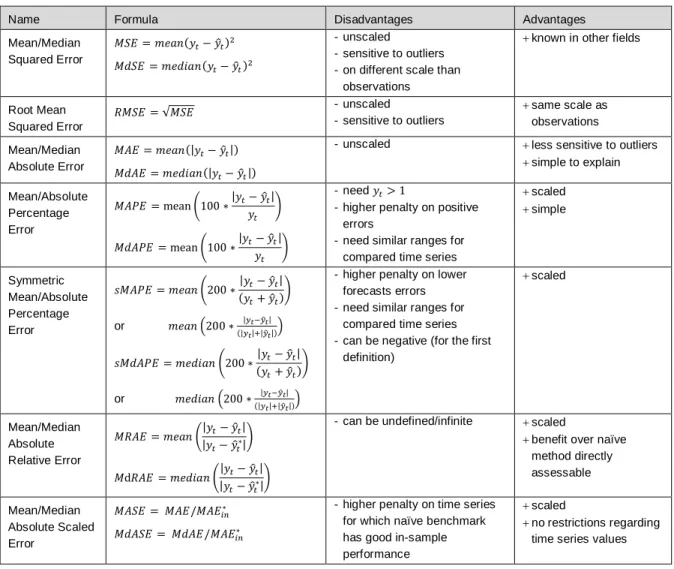
A vast bunch of metrics for measuring continuous target forecast performances exist and often make the results of forecast benchmarks confusing due to different rankings for different metrics, additionally depending on the forecast horizon (cf. Makridakis & Hibon (2000)). Due to this fact, it is absolutely important to understand the advantages, disadvantages and pitfalls of the commonly used metrics in order to avoid misleading benchmark results influencing the decision for an algorithm as well as false assessment of the benefit a forecasting method can provide. The best reference for this often overlooked fact is Hyndman & Koehler (2006). The following explanations are highly influenced by this resource adding some important points not mentioned there.

See also Table 2.1 summarizing the main performance metrics together with their advantages and disadvantages.

The first group discussed is about scale-dependent measures. The most popular metric form this

group due to some optimality properties in classical regression is the Mean Squared Error 𝑀𝑆𝐸 =

𝑚𝑒𝑎𝑛(𝑦𝑡− 𝑦̂𝑡)2. Notice that the mean operator here usually stands for the mean of squared forecast

errors over the horizons, e.g. 𝑚𝑒𝑎𝑛(𝑦𝑡− 𝑦̂𝑡)2=

1

ℎ∑ (𝑦𝑡− 𝑦̂𝑡) 𝑇+ℎ

𝑡=𝑇+1 , but can as well be used for the

(20)

2 Prerequisites

1

𝑆∑ (𝑦𝑖− 𝑦̂𝑖) 2 𝑆

𝑖=1 . Even though the first version is mostly meant, this double usage can lead to some

confusion as further explained below. In order to have the metric on the same scale as the

observations, also the Root Mean Squared Error 𝑅𝑀𝑆𝐸 = √𝑀𝑆𝐸 is used. A more outlier insensitive

measure represents the Mean Absolute Error 𝑀𝐴𝐸 = 𝑚𝑒𝑎𝑛(|𝑦𝑡− 𝑦̂𝑡|) or an even more robust version,

the Median Absolute Error 𝑀𝐴𝐸 = 𝑚𝑒𝑑𝑖𝑎𝑛(|𝑦𝑡− 𝑦̂𝑡|).

All these measures are not appropriate for comparing or aggregating results for time series with different scales (e.g. time series ranging between 1-2 and 1-1000). And it is very uncommon for time series to be initially scaled in order to circumvent this problem. Furthermore this would not solve the problem if the train and test fold are on a different scales already for a single time series due to a trend or increasing seasonality for instance. Though, for same scaled series like the data sets of the NN5 competition representing daily ATM withdrawals, these measures make sense.

The usual approach to tackle different scaled data is the usage of measures based on percentage errors. The most popular representative from this group is the Mean Absolute Percentage Error

𝑀𝐴𝑃𝐸 = 𝑚𝑒𝑎𝑛(100 ∗ |𝑦𝑡− 𝑦̂𝑡| 𝑦⁄ )𝑡 with the more robust version taking the median, resulting in MdAPE

(Median Absolute Percentage Error). To use this metric, one must assure that the time series are strictly positive or even assure it to only have responses greater than 1 in order to avoid excessively

Name Formula Disadvantages Advantages Mean/Median Squared Error 𝑀𝑆𝐸 = 𝑚𝑒𝑎𝑛(𝑦𝑡− 𝑦̂𝑡)2 𝑀𝑑𝑆𝐸 = 𝑚𝑒𝑑𝑖𝑎𝑛(𝑦𝑡− 𝑦̂𝑡)2 - unscaled - sensitive to outliers - on different scale than

observations

 known in other fields

Root Mean Squared Error 𝑅𝑀𝑆𝐸 = √𝑀𝑆𝐸 - unscaled - sensitive to outliers  same scale as observations Mean/Median Absolute Error 𝑀𝐴𝐸 = 𝑚𝑒𝑎𝑛(|𝑦𝑡− 𝑦̂𝑡|) 𝑀𝑑𝐴𝐸 = 𝑚𝑒𝑑𝑖𝑎𝑛(|𝑦𝑡− 𝑦̂𝑡|)

- unscaled  less sensitive to outliers

 simple to explain Mean/Absolute Percentage Error 𝑀𝐴𝑃𝐸 = mean (100 ∗|𝑦𝑡− 𝑦̂𝑡| 𝑦𝑡 ) 𝑀𝑑𝐴𝑃𝐸 = mean (100 ∗|𝑦𝑡− 𝑦̂𝑡| 𝑦𝑡 ) - need 𝑦𝑡> 1

- higher penalty on positive errors

- need similar ranges for compared time series

 scaled  simple Symmetric Mean/Absolute Percentage Error 𝑠𝑀𝐴𝑃𝐸 = 𝑚𝑒𝑎𝑛 (200 ∗|𝑦𝑡− 𝑦̂𝑡| (𝑦𝑡+ 𝑦̂𝑡) ) 𝑠𝑀𝑑𝐴𝑃𝐸 = 𝑚𝑒𝑑𝑖𝑎𝑛 (200 ∗|𝑦𝑡− 𝑦̂𝑡| (𝑦𝑡+ 𝑦̂𝑡) ) or 𝑚𝑒𝑎𝑛 (200 ∗ |𝑦𝑡−𝑦̂𝑡| (|𝑦𝑡|+|𝑦̂𝑡|)) or 𝑚𝑒𝑑𝑖𝑎𝑛 (200 ∗ |𝑦𝑡−𝑦̂𝑡| (|𝑦𝑡|+|𝑦̂𝑡|))

- higher penalty on lower forecasts errors - need similar ranges for

compared time series - can be negative (for the first

- can be undefined/infinite  scaled

 benefit over naïve method directly assessable Mean/Median Absolute Scaled Error 𝑀𝐴𝑆𝐸 = 𝑀𝐴𝐸/𝑀𝐴𝐸𝑖𝑛∗ 𝑀𝑑𝐴𝑆𝐸 = 𝑀𝑑𝐴𝐸/𝑀𝐴𝐸𝑖𝑛∗

- higher penalty on time series for which naïve benchmark has good in-sample performance

 scaled

 no restrictions regarding time series values

Table 2.1: Main performance metrics in time series forecasting with advantages and disadvantages

(21)

2.3 Performance Analysis for Time Series Forecasting

high metric values. Furthermore this type of metric have the disadvantage to put a higher penalty on

positive errors 𝑦𝑡− 𝑦̂𝑡 than on negative errors (assuming the average of 𝑦𝑡 and 𝑦̂𝑡 is the same); e.g.

think of a forecast value of 𝑦̂𝑡= 2 for a real value of 𝑦𝑡= 1 and vice versa resulting in percentage

errors of 100 and 50 respectively. To tackle the latter problem the Symmetric Mean Absolute

Percentage Error 𝑠𝑀𝐴𝑃𝐸 = 𝑚𝑒𝑎𝑛(200 ∗ |𝑦𝑡− 𝑦̂𝑡| (𝑦⁄ 𝑡+ 𝑦̂𝑡)) was invented together with its robust

counterpart sMdAPE using the median. Now the measure is symmetric regarding positive and

negative errors but not regarding high and low forecasts. E.g. a forecast of 𝑦̂𝑡= 3 for a value 𝑦𝑡= 2

results in 𝑠𝑀𝐴𝑃𝐸 = 40 whereas 𝑦̂𝑡= 1 leads to 𝑠𝑀𝐴𝑃𝐸 = 66.6, putting a higher penalty on lower

forecasts. This problem also resists the adaption of using absolute values in the denominator (𝑚𝑒𝑎𝑛(200 ∗ |𝑦𝑡− 𝑦̂𝑡| (|𝑦⁄ 𝑡| + |𝑦̂𝑡|))) to avoid negative sMAPE values due to negative forecasts.

One further problem occurs when the range (maximum-minimum) of different series in the test fold is similar but the minima highly differ. Actually this pitfall is equal to the one regarding values near zero already mentioned above. For example, a time series ranging between 1001-1002 in the test fold (not

uncommon for time series with a trend) produces a sMAPE of 𝑜(10−3₎_{whereas a time series with a}

range of 1-2 results in 𝑜(1). This situation is also happening for the Tourism and the M3 competition

data and even occurs less severe for the simulated Arimasim data. Again the NN5 series do not suffer from this problem as all series are on the same scale and have similar ranges.

All above problems are circumvented by a different type of scaling utilized by metrics based on relative errors. Here each forecast error is scaled by its counterpart from a benchmark method usually the

naive (taking last value) or snaive (seasonal naïve: taking last seasonal value) forecast. Unfortunately

the Mean Relative Absolute Error 𝑀𝑅𝐴𝐸 = 𝑚𝑒𝑎𝑛(|𝑦𝑡− 𝑦̂𝑡| |𝑦⁄ 𝑡− 𝑦̂𝑡∗|) (with 𝑦̂𝑡∗ denoting the forecast

from the benchmark method) can be undefined in case of a perfect fit of the benchmark method leading to a denominator of zero. If this happens in the analysis of this thesis, the NA (not applicable) value is used as a replacement. Even though assuming an infinite metric value in this case and applying the robust version using the median MdRAE does only help when multi-horizon forecast are aggregated by this measure (and the naïve forecast does not perfectly fit the majority of horizons) or when summarizing over time series instead of forecast horizons (and the naïve forecast does not perfectly fit the majority of series). On the other hand, a nice feature of this metric is that one can get the information that the chosen method is x% better on average (using mean or median for averaging) than the naïve method which is a very helpful information for evaluating the benefit against the effort of the non-naïve method.

A third alternative for scaling performance metrics avoiding all described disadvantages so far, was

invented by Hyndman & Koehler (2006). The Mean Absolute Scaled Error

𝑀𝐴𝑆𝐸 = 𝑚𝑒𝑎𝑛 (|𝑦𝑡− 𝑦̂𝑡| ( 1

𝑇−1∑ |𝑦𝑖− 𝑦𝑖−1| 𝑇

𝑖=2 )

⁄ ) scales every error by the in-sample MAE (which is the

mean of the 1-step-ahead in-sample errors) of the naïve forecast: 1

𝑇−𝑚∑ |𝑦𝑖− 𝑦𝑖−1| 𝑇

𝑖=𝑚+1 . The formula

for the MASE can also be written as 𝑀𝐴𝑆𝐸 = 𝑀𝐴𝐸/𝑀𝐴𝐸𝑖𝑛∗ with 𝑀𝐴𝐸𝑖𝑛∗ denoting the in-sample MAE of

the naïve benchmark. It is important to notice that the counterpart using the median instead of the

mean is restricted to the nominator, i.e. 𝑀𝑑𝐴𝑆𝐸 = 𝑀𝑑𝐴𝐸/𝑀𝐴𝐸𝑖𝑛∗. The only disadvantage also popping

up in the Tourism forecasting competition and commented on Hyndman (2015b), is that the “MASE

can be very sensitive to a few series [i.e. the ones with a small 𝑀𝐴𝐸_𝑖𝑛∗_{], and to optimize MASE [in a}

competition] it is worth concentrating on these”.

Somewhat between the scaled metrics based on relative errors and metrics based on scaled errors, which also preserves the nice comparison feature related to the naïve benchmark, is the Relative

Mean Absolute Error 𝑅𝑒𝑙𝑀𝐴𝐸 = 𝑀𝐴𝐸/𝑀𝐴𝐸∗_(with_𝑀𝐴𝐸∗_{denoting the already aggregated MAE of the}

benchmark method). Obviously one can use arbitrary performance metrics in the ratio in order to compare the desired measure with the benchmark value, resulting in RelRMSE, RelMAPE, etc.

(22)

2 Prerequisites

Similar to this approach, as also comparing just the final metrics, are rankings. Here several (including naïve methods) algorithms are assigned ranks due to their performance (measured by any of the metrics shown in Table 2.1). The latter is highly used in the benchmark tests of this thesis as explained below.

It is generally important to use different naïve benchmarks when conducting such comparisons. For

the analyses of this thesis not only the seasonal naïve (snaive) is used but also two approaches to

account for a possible trend by tsnaiveD and tsnaiveSTL. The first one is applying a seasonal

differencing and assumes a random walk with drift for the differenced series; see Chapter 3.1.1 for an explanation of differencing and the random walk with drift model. The second one is doing the same but accounting for seasonality by a STL decomposition (cf. Chapter 3.3). In fact both models assume that the time series can be best forecasted by a linear trend + seasonality + random variation. The

additional alternatives tsnaiveD_bc and tsnaiveSTL_bc apply an initial Box-Cox transformation (cf.

Chapter 3.1.1 for explanations of Box-Cox transformations) to account also for increasing seasonality.

In fact this last group of metrics (relative measures and rankings) is different from the former ones because of computing the comparison on already calculated performance metrics. But it makes the topic of time series performance metrics even more confusing as one always not only has to make clear for a benchmark study when and how (using mean or median) the aggregation over horizons is conducted in conjunction with the aggregation over different time series but also denote the point when different forecast algorithms are compared, e.g. by ranking, during this process.

Actually it is just the additional aggregation over different horizons, together with the known phenomenon that performances can differ from horizon to horizon, which makes interpreting time series benchmarks more complicated than standard benchmarks!

2.3.2 Performance Plots and Tables

For the benchmark studies of this thesis only the robust versions of sAPE, RAE and ASE, i. e. sMdAPE, MdRAE and MdASE, are used as outliers can occur just by chance due to the sheer amount of time series. Just for the NN5 data, a final comparison with the results of other authors is done on the basis of sMAPE as this was the target metric in the competition. Already note that a direct quantitative comparison with the results of the Tourism competition (with MASE as the evaluation metric) is not possible as the test data was not available (see also Chapter 2.1). Also for M3 only a qualitative comparison with the competition results can be given partly due to the reduction to series comprising more than 120 time points in this thesis (see below).

As an exception, the MAE is suitable for the simulation study in Chapter 4.5 as the predictions from different models are all comparable and do not contain outliers.

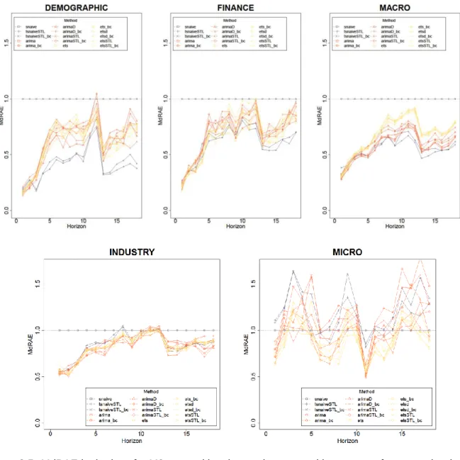
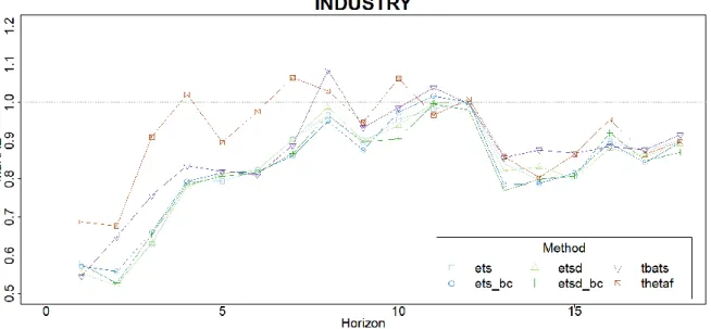
The main shortage which prohibits a comparison with quantitative M3 results is that these are presented in Makridakis & Hibon (2000) just on an overall aggregated level (over all time series) even though forecastability according the different categories highly differs! This can be nicely illustrated by a lineplot showing for example how the MdRAE, aggregated over all series of a category, evolves by

horizon. This is done in Figure 2.5for a bunch of classical (explained in Chapter 3) and naïve models.

Remarkably DEMOGRAPHIC and FINANCE tagged time series show a similar behavior regarding the

forecast performance of the methods. Especially for the MACRO time series, the “ets” tagged models

show an inferior performance. For these three categories a clear improvement to a seasonal naïve

model (grey line, constant due to plotting the relative to snaive forecast error) results. But when

comparing to the tsnaiveSTL based models the dominance disappears at least after half of a season

(23)

+ random variation and can be best forecasted by a deseasonalized random walk with drift which is

the forecast technique behind tsnaiveSTL. This fact makes any benchmarking of sophisticated models

for these time series highly questionable!

For the two remaining categories INDUSTRY and MICRO the situation is different, showing a better

forecast performance than the naïve methods even though the classical models for the MICRO time

series exhibit a very special shape, kind of alternating between better and worse than seasonal naïve forecasts emphasizing again the importance of distinguishing also these two categories. This alternating behavior can also be found for the Tourism competition data (not shown here), leaving the

INDUSTRY data sets as the only interesting time series from the M3 competition that are eligible to reveal additional insights.

Due to these findings any further comparison for M3 data is restricted to INDUSTRY tagged time

series which is by chance also the category comprising most of the competition data sets. For reasons

of completeness the results for DEMOGRAPHIC, FINANCE, MACRO and MICRO are compactly put

into the Appendix.

Figure 2.5:MdRAE by horizon for M3 competition time series grouped by category for some classical

(24)

2 Prerequisites

The dominant method for evaluating the overall performance between algorithms in this thesis is a Ranking based on the MdASE metric. The metric is calculated for every model according a special horizon range and subsequently a ranking of the models per time series is done. This ranking is then aggregated over time series and displayed by a boxplot which allows also a visual impression of the variability of the performance. The horizon range typically comprises h=1 (1-step-ahead forecast), at least the first season and the largest range which is usually the competition objective, nicely summarizing the most informative time areas, even though alternatively this analysis can be conducted for every season (or half season) individually for instance. For example, for the NN5 data

the latter would exhibit the performance boost in the 3rd week due to Easter effects for the models

using covariates.

Figure 2.6 shows an example, plotting the MdASE for some naïve methods together with some

classical approaches for the Tourism data. As the top performing models are often close, an additional tabulation of the mean ranks is usually given, underlining the best metric per horizon. Additionally shading the TopX% helps in identifying the runner-ups (see Table 2.2).

Figure 2.6: Ranked MdASE by horizon range of some naïve and classical forecast models for

Tourism competition data.

Method Tourism h=1-1 Tourism h=1-6 Tourism h=1-12 Tourism h=1-24 Method Tourism h=1-1 Tourism h=1-6 Tourism h=1-12 Tourism h=1-24 snaive 9.35 8.54 9.48 9.82 arimaSTL 8.84 10.41 10.18 10.04 tsnaiveD 9.27 7.94 8.24 8.27 arimaSTL_bc 8.76 8.11 7.84 8.00 tsnaiveD_bc 9.79 8.49 8.64 8.98 ets 9.01 8.50 8.42 8.46 tsnaiveSTL 9.96 11.68 11.85 11.46 ets_bc 9.25 9.20 9.10 8.92 tsnaiveSTL_bc 9.66 9.36 10.09 10.10 etsd 9.07 8.42 8.58 8.58 arima 8.05 9.03 8.56 8.68 etsd_bc 9.35 9.66 9.45 9.16 arima_bc 8.42 8.57 8.49 8.58 etsSTL 9.14 11.01 10.44 10.29 arimaD 7.76 7.85 7.68 7.48 etsSTL_bc 9.19 8.79 8.35 8.41 arimaD_bc 8.14 7.44 7.62 7.77

Table 2.2: Average Ranked MdASE corresponding to dots in Figure 2.6. Best model metric per

horizon range (with vertical split just for visual convenience) is bold & underlined and shading denote Top20% accordingly.

(25)

When using a different robust metric, the results can change, but usually not very extreme on a qualitative scale. This also holds when switching to unrobust measures as the ranking per time series kind of robustifies the performance metrics again. Obviously the situation changes when just reporting e.g. the unrobust MASE averaged over all time series without the intermediate ranking! Something

similar happens for the NN5 benchmark using the 4th best method (of 226) according ranked MdASE

to outperform all competition competitors when using the competition objective metric, i.e. sMAPE (see Chapter 5.3).

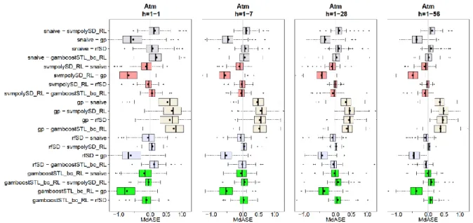
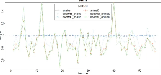
The boxplots in Figure 2.6 exhibit a special shape, i.e. a left skewed form for methods better than the average and right skewed for the other half. This is due to the fact that also the best overall method is also under the worst for some benchmark time series and vice versa which can already be seen by the whiskers comprising the whole range of ranks. This circumstance further indicates that also a paired comparison of performance metrics will not reveal more information which theoretically can happen as one deals with paired measures. Actually it might happen that even the boxplots of two methods highly overlap their paired metric difference shows a more distinct behavior. To evaluate this possibility one can plot the paired metric differences like in Figure 2.7 showing results for some selected models (for explanations of these models see the forthcoming chapters). More precise, these

models are the seasonal naïve (snaive); the best model according MdASE and the whole test horizon

h=1-56 named svmpolySD_RL; the according worst model gp and two medium performant

approaches rfSD and gamboostSTL_bc_RL. Actually this plot exhibits some typical behavior that often

occurs in time series forecasting benchmarks. First of all, it can be seen that the snaive beats any of

the other models (including the winner svmpolySD_RL) at all horizon ranges for some time series.

More striking is the fact that this holds mostly also for the worst model gp. Furthermore it can be seen

that for the 1-step ahead forecast the gamboostSTL_bc_RL is better than the overall winner

svmpolySD_RL but drastically loosing when compared on the whole horizon range h=1-56. This gets

more remarkable when comparing the gamboostSTL_bc_RL with the rfSD model that improves its

forecast performance the wider the horizon range is and therefore showing an opposite behavior regarding horizon related change.

Figure 2.7: Differences of MdASE (“MdASE of left model – MdASE of right model”) by horizon range

(26)

2 Prerequisites

It must be added that above demonstrated “performance overlap” is even worse for the Tourism and M3 competition due to the models being less differentiating regarding the forecast performance and as well because of dealing with more time series compared to NN5!

Together with above findings regarding differing rankings for different metrics, the no-free-lunch theorem stating that there is no best predictive model for all data must be enlarged when dealing with time series, indicating a dependency of the question for the best algorithm not only on the used metric but also on the horizon!

This has severe implications on the practical application of forecast models as the user must carefully define the objective regarding the desired horizon range. Also the performance metric should be sensibly chosen taking the results from Chapter 2.3.1 into account and simultaneously decide whether a robust or outlier-sensitive performance metric better suits the objective.

(27)

3 Classical Time Series Models

3.1 ARIMA and Friends

In the following the classical ARIMA model is explained together with extensions. A very handy introduction can be found in Ruppert (2010). Shumway & Stoffer (2011), on the other hand, is a more technical text book. As always, the book from Hyndman & Athanasopoulos (2014) has a nice introduction for the practitioner. Furthermore the blog entry “The ARIMAX model muddle” from Hyndman (2015b) is very helpful.

3.1.1 ARIMA

The classical ARIMA (autoregressive integrated moving average) approach tries to model a time

series by the autocorrelation due to the dependence of 𝑦𝑡 on former values. For example, an

autoregressive process of order p, named AR(p), models the current mean-centered target value by

(auto-)regressing it on its own past values 𝑦𝑡= 𝜙1𝑦𝑡−1+ ⋯ + 𝜙𝑝𝑦𝑡−𝑝+ 𝑤𝑡 with 𝑤𝑡 denoting a white

noise process, i.e. a family of uncorrelated, not necessarily independent (!), random variables with constant covariance and expected value equal zero. Mostly a Gaussian distribution is assumed which

in turn results in i.i.d. white noise. Using the autoregressive operator 𝜙(𝐵) = 1 − 𝜙1𝐵 − ⋯ − 𝜙𝑝𝐵𝑝, with

B denoting the backshift or lag operator (𝐵𝑝_𝑦

𝑡= 𝐵𝑝−1𝑦𝑡−1= ⋯ = 𝐵𝑦𝑡−𝑝+1= 𝑦𝑡−𝑝), above model

equation can be written more compact by 𝜙(𝐵)𝑦𝑡=𝑤𝑡.

An important concept for ARIMA modeling is weakly stationarity, which means that 𝐸(𝑦𝑡) = 𝜇𝑡= 𝑐𝑜𝑛𝑠𝑡.

and 𝛾(𝑡, 𝑡′) = 𝑐𝑜𝑣(𝑦𝑡, 𝑦𝑡′) = 𝛾(|𝑡 − 𝑡′|), i.e. the autocovariance is only dependent on the time difference

|𝑡 − 𝑡′|, including constant variance assumption (𝑡 == 𝑡′). This requirement not only leads to some

constraints for the possible coefficients 𝜙1..𝑝, e.g. |𝜙1| < 1 in case of an AR(1) process, but more

importantly, is at least needed to estimate the parameters 𝜙1..𝑝 from just one time series (as otherwise

not enough data is left for estimation).

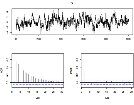
ACF and PACF

An important diagnostic tool for ARIMA modeling is the sample PACF (partial autocorrelation function) plot showing the direct influence, or correlation adjusted on the influence of intermediate points, of

𝑦𝑡−ℎ on 𝑦𝑡. Figure 3.1 shows an example of this plot together with the sample ACF (autocorrelation

function) plot denoting the unadjusted influence for a simulated AR(2) process. One can see that the PACF needles cut off after p=2 lags (apart from non-significant values) hinting to the correct number of coefficients, whereas in the ACF the coefficients die out slowly.

Apart from applying these plots to stationary data, they can also be used determining the relationship with lagged values in other modeling approaches, e.g. detecting seasonality by periodic ACF spikes or a significant PACF spike at the first seasonal lag. But one always has to keep in mind that these plots just visualize the linear correlation of time points and can therefore hide nonlinear relationships which would pop up when plotting the time point values against their lagged counterparts.

Sometimes data shows the opposite behavior compared to Figure 3.1: An ACF plot with just one or two significant lags and a PACF plot with out-dying lags. This cannot be modeled by an AR process as such a process always results in having some correlation to all past values. In order to model this parsimoniously, i.e. without estimating lots of (or infinite) AR-coefficients, a MA(q) (moving average) process is assumed where the current mean-centered value of the time series is modeled as a moving