Hierarchical Bayesian topic modeling with sentiment and author extension

(1)

HIERARCHICAL BAYESIAN TOPIC MODELING WITH SENTIMENT

AND AUTHOR EXTENSION

by

MING YANG

B.E., Nanjing University of Posts and Telecommunications, China, 2009

AN ABSTRACT OF A DISSERTATION

submitted in partial fulfillment of the

requirements for the degree

DOCTOR OF PHILOSOPHY

Department of Computing and Information Sciences

College of Engineering

KANSAS STATE UNIVERSITY

Manhattan, Kansas

(2)

Abstract

While the Hierarchical Dirichlet Process (HDP) has recently been widely applied to topic modeling tasks, most current hybrid models for concurrent inference of topics and other factors are not based on HDP.

In this dissertation, we present two new models that extend an HDP topic modeling framework to incorporate other learning factors. One model injects Latent Dirichlet Al-location (LDA) based sentiment learning into HDP. This model preserves the benefits of nonparametric Bayesian models for topic learning, while learning latent sentiment aspects simultaneously. It automatically learns different word distributions for each single sentiment polarity within each topic generated.

The other model combines an existing HDP framework for learning topics from free text with latent authorship learning within a generative model using author list information. This model adds one more layer into the current hierarchy of HDPs to represent topic groups shared by authors, and the document topic distribution is represented as a mixture of topic distribution of its authors. This model automatically learns author contribution partitions for documents in addition to topics.

(3)

HIERARCHICAL BAYESIAN TOPIC MODELING WITH SENTIMENT

AND AUTHOR EXTENSIONS

by

MING YANG

B.E., Nanjing University of Posts and Telecommunications, China, 2009

A DISSERTATION

submitted in partial fulfillment of the

requirements for the degree

DOCTOR OF PHILOSOPHY

Department of Computing and Information Sciences

College of Engineering

KANSAS STATE UNIVERSITY

Manhattan, Kansas

2016

Approved by: Major Professor William H. Hsu

(4)

Copyright

MING YANG

(5)

Abstract

While the Hierarchical Dirichlet Process (HDP) has recently been widely applied to topic modeling tasks, most current hybrid models for concurrent inference of topics and other factors are not based on HDP.

In this dissertation, we present two new models that extend an HDP topic modeling framework to incorporate other learning factors. One model injects Latent Dirichlet Al-location (LDA) based sentiment learning into HDP. This model preserves the benefits of nonparametric Bayesian models for topic learning, while learning latent sentiment aspects simultaneously. It automatically learns different word distributions for each single sentiment polarity within each topic generated.

The other model combines an existing HDP framework for learning topics from free text with latent authorship learning within a generative model using author list information. This model adds one more layer into the current hierarchy of HDPs to represent topic groups shared by authors, and the document topic distribution is represented as a mixture of topic distribution of its authors. This model automatically learns author contribution partitions for documents in addition to topics.

(6)

List of Figures

1.1 Graphical plate model of LDA . . . 5

1.2 Graphical plate model of HDP . . . 8

1.3 HDP: Chinese Restaurant Franchise Representation . . . 10

2.1 Example of topics and sentiment polarities in hotel reviews . . . 18

2.2 Plate model for HDP model with sentiment labels . . . 19

3.1 Example of topic modeling with author cooperation . . . 34

3.2 Plate Model for HDP model with authors . . . 38

3.3 Inference process for HDPauthor model . . . 49

4.1 Perplexity evolution for TripAdvisor experiments . . . 57

4.2 Perplexity evolution for DBLP experiments . . . 71

(10)

List of Tables

4.1 Table for four different topics from TripAdvisor reviews . . . 55

4.2 Evaluation measures for theTripAdvisorexperiment compared to LARA and baseline models . . . 56

4.3 Table for four different topics from Yelp Reviews . . . 58

4.4 Table for top conferences in computer science research areas . . . 61

4.5 Example of top topics learned from NIPS experiment . . . 68

4.6 Example of top topics for selected authors learned from NIPS experiment . . 69

4.7 Example of top topics learned from DBLP experiment . . . 72

(11)

Acknowledgments

I would like to thank all the people who have helped me during my Ph.D study here in Kansas State University for all these years.

First and Foremost, I would like to thank my advisor William H. Hsu. He is very helpful, knowledgeable, patient and enthusiastic. Dr. Hsu is very supportive, and has many brilliant ideas, I have learned a lot from him throughout my study under his supervision.

I also want to express my gratitude to all my committee members, Dr. Torben Amtoft, Dr. Xinming Ou, and Dr. Shing I Chang, for their suggestions and advice, which helped me a lot with this dissertation.

I also appreciate all the help from my colleagues in KDD (Laboratory for Knowledge Discovery in Databases) group, especially Wesam Elshamy, Surya Kallumadi, Joshua Weese, and many undergraduate students. I want to thank Qiaozhu Mei, Chong Wang, and Hongn-ing Wang, who helped me in various ways.

Last but not least, I want to thank all my family members for taking care of me and supporting me all the time.

(12)

Dedication

(13)

Chapter 1

Introduction

Nonparametric Bayesian topic model frameworks1 2_{, such as the Hierarchical Dirichlet}

Pro-cess (HDP)3_{, have been proven to work successfully and more accurately than other extant}

approaches such as latent semantic analysis (LSA)4_{, and its probabilistic analogue}5_{. HDPs}

have also been used directly and solely in many real-world applications. However, as a fundamental text analysis framework, extensions to HDP have not garnered much attention within the area of natural language processing.

In the real-world applications alluded to above, the topic extraction problem is always accompanied by other learning needs, such as sentiment analysis6_{, author identification}7_,

community detection8 9_{, and so on. To make full use of the benefits and advantages of}

the HDP topic inference framework, and in particular to learn a better hidden structure of documents, the synthesis of HDP with learning models from other text analysis studies deserves exploration.

Based on a deep investigation of topic modeling and the theoretical foundations of the HDP framework, this dissertation aims to extend HDP topic modeling framework to incor-porate sentiment analysis/author identification learning needs, to form hybrid text analysis models. These hybrid models can solve topic modeling and sentiment analysis/author iden-tification problems in the meantime.

(14)

The primary novel contribution of this work is the systematic and principled extension of HDP to incorporate sentiment and co-authorship as independent properties of document corpora, which we accomplish by synthesizing basic HDPs with generative formulations of sentiment and author components. We treat sentiment as a separate parameter to be paired with topic parameters, so that the full pair (dyad) of sentiment and topic condition-ally vary based on hyperparameters governing the disposition of a document author. This new approach allows us to capture sentiment-topic parameters within a holistic nonpara-metric Bayesian framework. Independently of this, we treat authors as participating entities represented within the traditional HDP mixture model, which we extend to capture authors as DP mixtures of global topics in which they have inferable expertise, and documents in corpora as finite mixture of its authors, in whose creation they have participated. This is the first sentiment-topic model we know of that incorporates sentiment as an orthogonal component of any such HDP-based hybrid topic model, and similarly the first HDP-based author-topic model.

The central thesis of this work is that extending the HDP using Latent Dirichlet Allo-cation (LDA), and similar nonparametric Bayesian formulations of sentiment and author components, allows straightforward extensions to accurately capture and infer meaningful sentiment-topic combinations, as well as useful author-topic distributions for imputation of author expertise. This can be empirically evaluated in our applications by looking at our prediction result for predefined categorical rating values from inferred topic-level sentiment result from our HDPsent model in domains such as product and service reviews, using fully unsupervised learning. Furthermore, we are also able to validate the posterior distribution of authors and attributed topics learned from ourHDPauthormodel in academic publication corpora by our performance on some retrieval tasks.

(15)

1.1

Topic Modeling

Since the rise of text-driven data mining and decision support in a wide variety of application domains such as recommender systems and personalized decision support, text analytics systems have been well-studied and developed. Topic modeling, as one major branch in this field, has been used in many domains, such as discovering and generating topics in global corpora, identifying and differentiating language patterns for different topics, and associating topics with documents. Topic models are also helpful in many natural language processing (NLP) subareas, including document summarization, generation, classification and organization, and in particular text-based information retrieval (IR) and information extraction (IE).

The major milestones in topic modeling are based on building probabilistic generative models10 11_{. This includes Probabilistic Latent Semantic Indexing (pLSI)}5_{, Latent Dirichlet}

Allocation (LDA)12_{, and nonparametric Bayesian hierarchical model - Hierarchical Dirichlet}

Process (HDP)3_.

These topic models have been proved to be powerful and robust for learning topics from corpus. Instead of classifying or clustering documents to separate categories, these models capture the underlying latent probabilistic mixing proportions of multiple categories for each document. For example, one document on bioinformatics may admit different proportions of topics such as ”biology”, ”data mining” and ”statistics”. Meanwhile, another document on social network analysis may represent a mixture of identifiable topics such as ”graph theory”, ”data mining” and ”statistics”. Global topics may be represented in multiple documents. This statistical mixture model does not only helps to identify topics for documents more accurately, but also improves the word distribution gathering for different topics.

(16)

1.1.1

Problem Definition

There are many ways of defining and solving the topic modeling problem. In this disser-tation, however, we focus only on probabilistic methods of constructing statistical mixture models to simulate a generative process of text for documents.

From this point of view, in topic modeling, we generally define and use word sequences in text collection as data to analyze. Therefore, in the text collection, we only use words

as the basic unit of the data set, representing its granularity. We ignore the punctuation in documents, the sentence structure of words, as well as the part-of-speech (POS) tagging of words.

Here we define the following terms:

1. Each distinct word is treated as one distinct variable in data set, denoted as w. The set of all distinct words in whole text collections is denoted as vocabularyW with size

V. For simplicity, we index each word in vocabulary beforehand as W = {1, ..., V}, and then represent each word by its index id.

2. Each document in collection is considered to be represented by an array ofN words, re-gardless of punctuation and non-word characters. It is denoted asdj ={xj1, xj2, ..., xjN}.

Variable xji represents the ith word token in jth document, whose value should be

one w ∈ {1, ..., V}. Although we refer to each variable xji by its position, we here

assume that each token is generated independently from all other tokens in this docu-ment, given the generative model. Therefore, the order of word tokens in a document does not matter. And we also assume that each document is generated independently from all other documents, so that the order of documents in text collection does not matter, too. This exchangeability feature allows us to treat each document as a bag of words (BOW), which means that the positions of words in same document are interchangeable, and the positions of documents are also interchangeable.

(17)

corpus, which represents the set D={d1, d2, ..., dm} .

1.1.2

Latent Dirichlet Allocation

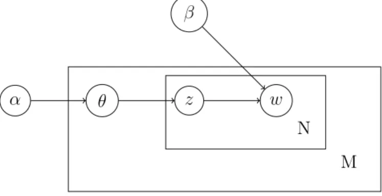
Latent Dirichlet Allocation (LDA) was introduced by Blei12 and is a widely used generative statistical model of text collection. Instead of directly producing multinomial distributions of words in topics, and multinomial distributions of topics in each document, LDA brings in the Dirichlet distribution as a conjugate prior for these multinomial distributions.

This model defines a hierarchical Bayesian model for generative process for word tokens in text. Here we represent a graphical plate model of LDA generative process in figure 1.1:

α θ z w

β

N M

Figure 1.1: Graphical plate model of LDA

This model predefines K topics in a corpus, and then associates each word with one latent topic variablez, wherez ∈ {1, ...K}. Therefore documentj that is originally denoted as dj ={xj1, xj2, ..., xjN} can also be represented by this sequence of latent topic variables

dj ={zj1, zj2, ..., zjN}, which is sampled according to the multinomial probability

distribu-tion over topic categories for this document, denoted πj = {πj1, ..., πjK}. We also assume

that each topic k is associated with a multinomial probability distribution over the whole vocabulary W with word sizeV, denoted asφk={φk1, ..., φkV}.

Since multinomial distributions can have Dirichlet distributions as prior parameters, In this model we makes use of this feature, and assume that the topic distributions for documents {π1, ..., πm} all have Dirichlet distributionDir(α) as their conjugate prior. And

(18)

the word distributions for topics {φ1, ..., φK} have Dirichlet distribution Dir(β) as their

conjugate prior.

The generative process of LDA for word tokens can be represented as follows:

1. For each topic k, we sample φk ∼Dir(β).

2. For each documentdj, we sample πj ∼Dir(α).

3. For each token xji in documentdj at positioni:

(a) We sample a latent topic label zji ∼M ultinomial(πj).

(b) We sample a word w∼M ultinomial(φzji).

The inference part of the LDA model is complex, since it involves posterior distribution calculation of latent variables θ and z generated by LDA model for documents, given the observed data w and prior hyper parameters α and β:

p(θ, z|w, α, β) = p(θ, z, w|α, β)

p(w|α, β) (1.1)

This posterior distribution is unable to compute directly, so that the exact inference of LDA model is intractable. There are two major algorithms applied widely for approximate inference of LDA, Variational Inference13 and Gibbs Sampling14.

Here we introduce the inference process using Gibbs sampling algorithm. Gibbs sampling does not require to infer latent parameters θ and φ explicitly. These parameters can be integrated out through the assignment of z.

According to the definition of Gibbs sampling, we do not need to sample all latent variables in whole data set {z11, z12, ..., zmN−1, zmN} together, whose joint probability is

actually intractable. We can sequentially sample each z based on values of all otherz. Thus, following Griffiths14_{, the conditional posterior distribution of} _z

ji given values of

(19)

p(zji =k|z−ji,w, α, β)∝p(wji|zji =k,z−ji,w−ji, β)p(zji =k|z−ji, α) (1.2)

where z−ji ₌_{_z

j0_i0|j0i0 6=ji} and w−ji ={w_j0_i0|j0i0 6=ji}.

In this equation, however,p(zji =k|z−ji, α) can be treated as a predictive new samplezji

from multinomial distributionθj withDir(α) as its conjugate prior, and z−jias its observed

data set. To calculate this predictive posterior distribution of variablezji, we can infer that:

p(zji =k|z−ji, α) =

n−_jkji+α

n−_j_·ji+Kα (1.3)

Similarly, p(wji|zji =k,z−ji,w−ji, β) can also be deemed as a predictive new sample of

wji from multinomial distribution φk with Dir(β) as its conjugate prior, z−ji and w−ji as

its observed data set. We can similarly infer that:

p(wji|zji =k,z−ji,w−ji, β) =

n−_kwji+β

n−_k_·ji+W β (1.4)

Putting equations1.3 and1.4 together, we can easily get the conditional sampling prob-ability p(zji =k|z−ji,w, α, β). Then we can directly use Gibbs sampling schema to sample

each z sequentially until the Markov chain converges and reaches a stable state.

1.1.3

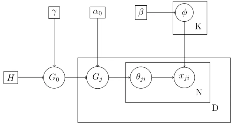
Hierarchical Dirichlet Process

The hierarchical Dirichlet process (HDP) is a widely used generative model for topic learning. HDPs were introduced by Teh3 _{and are a type of nonparametric hierarchical Bayesian model.}

One of its most favorable features is that the number of topics that a user has to set up beforehand is not directly bounded, but only regulated by a prior probability of generating a new topic.

The graphical plate model corresponding to HDP mixture model is shown in figure 1.2: In this model, H can be treated as a prior distribution over topics. It defines a global

(20)

H γ G0 α0 Gj θji xji β φ K N D

Figure 1.2: Graphical plate model of HDP

measure G0 for the whole corpora as a Dirichlet Process with H as base measure, and γ as concentration parameter. For each document dj in this corpora, it generates its own

probability distribution Gj over topics as Dirichlet Process with G0 as base measure, and

α0 as concentration parameter. Then the topic labelθji is sampled fromGj, word token xji

then is generated similarly to LDA according to its topic label.

The two-level hierarchical Dirichlet process mixture model can be represented as:

G0|γ, H ∼DP(γ, H)

Gj|α0, G0 ∼DP(α0, G0) for each j,

θji|Gj ∼Gj for each j and i,

xji|θji ∼F(θji) for each j and i,

(1.5)

Since exact inference over HDPs is also intractable, this model also contains two widely used approximate inference techniques, Variational Inference15 16and Gibbs Sampling3 as a special form of Markov chain Monte Carlo (MCMC) algorithm. HDP usesChinese restau-rant franchise as a representation framework for building posterior distribution of latent variables for Gibbs Sampling. Although Gibbs sampling is not as computationally efficient

(21)

or easy to be scaled as variational inference, it is one more accurate and unbiased way for parameter estimation, and it is also widely used in many applications.

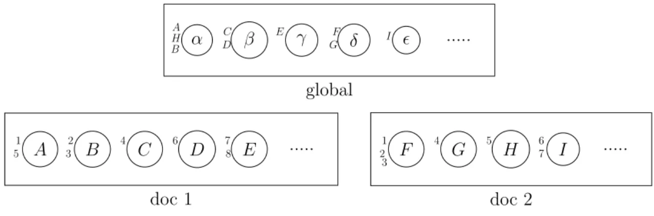
According to Chen17_{, with the representation framework of} _{Chinese restaurant}

fran-chise3_{, the generative process of HDP for word tokens can be represented as follows:}

1. Draw an infinite number of topics φk ∼Dir(β) fork ={1,2,3...}.

2. Draw stick-breaking topic proportions as νk ∼Beta(1, γ) for k ={1,2,3...}.

3. For each documentdj:

(a) we sample document-level topic atoms kjt ∼ M ultinomial(σ(ν)) for each table

t={1,2,3...}.

(b) we then sample document-level stick-breaking proportions as πjt ∼ Beta(1, α)

for each table t={1,2,3...}.

(c) For each token xji in document dj at position i:

i. We sample a latent topic label zji ∼M ultinomial(σ(πj)).

ii. We sample a word w∼M ultinomial(φzji).

Here σ(ν) andσ(πj) are distributions constructed by stick-breaking algorithm18 19 with proportions of ν ={νk|k = 1,2,3, ...} and πj ={πjt|t= 1,2,3, ...}as:

σk(ν) =νk k−1 Y i=1 (1−νi) σt(πj) =πjt t−1 Y i=1 (1−πji) (1.6)

Thus the Chinese Restaurant Franchise Process20 _{could be represented in Figure} _1.3_:

1.1.4

Markov Chain Monte Carlo and Gibbs Sampling

(22)

A B C D E ... 1 2 3 4 5 6 7 8 doc 1 F G H I ... 1 2 3 4 5 6 7 doc 2 α β γ _δ ... A B C D E F G H I global

Figure 1.3: HDP: Chinese Restaurant Franchise Representation

Monte Carlo (MCMC) framework21 22, it is also worth writing about the basic theories of this approximate inference technique.

Monte Carlo Integration23 makes use of Law of large numbers24. It approximates the integral of a complex function by a sample mean. We assume that X is a random variable that draws from a probability distribution π(·). If we want to calculate the expectation of function f(x) given probability distribution of x as π(·), then we can get:

E[f(X)] = R f(x)π(x)dx R π(x)dx ≈ 1 N N X i=1 f(xi) (xi ∼π(·)) (1.7)

However, in some cases, it is difficult or impossible to draw samples directly and in-dependently from a complex probability distribution. One way to solve this problem is to construct a Markov chain25_{whose stationary distribution is}_π₍_·_{) and then sample a sequence}

of random variables{x1, x2, ..., xN}through this Markov chain. Each state in Markov chain

is a variable value, which is sampled from last sample value using transition function. Gibbs Sampling is one algorithm developed from MCMC method. It is a special case of Metropolis-Hastings algorithm26 _{from MCMC. It is always used for solving the sampling}

problem of a multivariate probability distribution, while the joint probability of the set of variables in intractable.

(23)

Assume that the random variable X we want to sample is a k-dimensional multivariate variable as X = {X1, X2, ..., Xk} while its joint probability p(X) = p(X1, X2, ..., Xk) is

infeasible to compute directly. Instead, we can sample component variable i of X in jth sample xji from its conditional probability on all the other variable as

p(xji|xj1, xj2, ..., xji−1, xj−1i+1, ..., xj−1k) (1.8)

Thus, in Gibbs Sampling, each multivariate variable X is sampled by sequentially sam-pling each of its component variables, conditionally on current values of all other variables.

1.2

Sentiment-Topic Model:

HDPsent

One research area closely related to topic modeling is sentiment analysis, which refers to the uses of text for learning the underlying polarity (positive or negative tone) and subjec-tive attitude of author (or authors) of documents. Early approaches towards using machine learning to detect the overall sentiment polarity of text documents used basic supervised in-ductive learning for classification. Hypothesis languages and learning algorithms underlying such techniques include Naive Bayes, Maximum Entropy, and Support Vector Machines, as applied by Pang27 6 and Liu28.

Compared to overall sentiment polarity learning, however, detailed sentiment polarity learning combined with topics is more favorable. Topic learning embedded into sentiment analysis provides users and researchers with a hybrid model for simultaneous topic distribu-tion and sentiment polarity analysis of documents. Moreover, it also helps to enhance the ability for isolating sentiment polarities from different topics in same document, and pro-vides with the ability to infer separate aspect-level sentiment clusters with different word distributions.

There are some benefits and advantages we can gain from a hybrid topic sentiment model. By modeling sentiment analysis along with topic learning under HDP framework, we are not

(24)

restricted by predefined topic size. We can not only discover new topics representing different data groups, but also form sentiment word clusters under each of the topics generated.

Furthermore, we can identify different word distributions with same sentiment polarity under different topics, as well as differentiate same word with different sentiment polarities on different topics. This flexibility improves our ability of learning topic and sentiment combination clusters across the whole corpora more precisely, also improves our ability of identifying the aspect-level sentiment polarities on different topics in one document.

1.3

Author-Topic Model:

HDPauthor

Another extension of topic modeling is to incorporate author identification information within documents into the learning process.

This research problem consists of several key technical objectives, one of which is to identify topic interests for each author according to the documents that one participates in. For documents finished by cooperation of a set of authors, we also want to learn the contribution for each author involved in this document. Moreover, author identification information itself can be very helpful as a supporting learning resource for topic learning of documents. By constructing global topic interests of authors across corpora, knowledge of authorship can help us to learn topics for documents better. Finally, by computing the topic distribution of all documents that same author participates in, the topic interests of this author can be more accurately inferred as well.

Besides topic learning for documents and authors, our HDPauthor model also achieves learning of mixing proportions for authors of each document. The learning result can be used directly for estimation of author contribution.

Examples of applications of topic and author mixture learning model include author identity disambiguation problem. In scientific publications, distinct authors frequently have the same name. There are also some authors who show up in different papers with

(25)

dif-ferent names due to variations in abbreviation. Incorporating the feature of topic interest distributions for authors would help us to alleviate this disambiguation problem.

While author searching, grouping, ranking and recommendation are useful tools in many document/author retrieval applications, the topic interests of authors learned from this model also provide features for direct similarity comparison between different authors, using other advanced machine learning techniques.

1.4

Road Map

This dissertation aims to cover two hybrid inference model as extension of HDP topic learn-ing framework. The chapters are organized as follows:

In Chapter 2, we present one novel hybrid learning approach based on the existing HDP topic learning framework, which combines topic modeling with sentiment analysis within one generative inference process. This model preserves the benefits of nonparametric Bayesian models for topic learning, while learns latent aspect-level sentiment features for each topic generated simultaneously.

In Chapter 3, we introduce one novel model that extends the current HDP topic model to incorporate author cooperation information. This model infers topic interests of each author involved in a corpus first, and then establishes the topic distribution of each document in the corpus as a finite mixture of the topic interest of all its authors. This model not only manages to learn topics for documents, and topic interests for each author, but also is able to learn author contributions for each document.

In Chapter 4, we describe in detail the data sets we gathered from real-world text for experiments on our models. We also introduce the criteria we use for evaluation of these experiments. We then describe our experiments and document results that we collected from them.

(26)

review remaining open problems and some research directions regarding these models that we propose to explore in future work.

(27)

Chapter 2

Sentiment-Topic Model:

HDPsent

With the growing need for analyses of free text that extract both feature information and sentiment polarity, hybrid probabilistic models that support concurrent topic and sentiment analysis have also increased in relevance and significance. Many models treat topic modeling and sentiment analysis as separate and independent processes, which lacks the ability for isolating sentiment polarity from different topics. We would like to infer the topics of documents, but also want to infer the sentiment information for these topics.

There are some algorithms which already attempt to build a hybrid inference model for topic and sentiment learning29 30_{, but these models do not fully make use of the current}

state of the field in nonparametric Bayesian HDP models as a representational framework. For example, when we analyze product or service reviews, it is crucial that we have sep-arate sentiment polarity information for each feature aspects, which helps us to differentiate opinion words for different aspects from one review text. This, in turn, extends our ability for feature-specific sentiment polarity analysis.

In this chapter we present a technique for simultaneously inferring sentiment and topic from free text, extending existing HDP models, called HDPsent. Our model is the first to extend the existing HDP model by adding a sentiment label l along with a topic label

(28)

implementations of the Chinese restaurant franchise process (CRFP) for the generative HDP model.

2.1

Related Work

Some significant work in the past decade has begun to combine topic modeling and sen-timent analysis in a single model. In applications of the Topic Sensen-timent Mixture Model (TSM)30, a Probabilistic Latent Semantic Analysis (PLSA) model is used to represent the generative process. Furthermore, even it assigns topic label for each word (excluding back-ground words), that word itself is sampled from either general positive, negative model, or that specific topic model. This generative process generalizes sentiment polarity model and has limited ability to make different sentiment polarity word distributions for different topics. However, our intuition is that different topics might treat same words with different sentiment strength, or even different polarity. For example, the word ”small” might be a positive word when it is describing the size of a MP3 player, but might be a negative word when it is describing the storage capacity of that MP3 player. One approach to handling this problem is word sense induction31, which is beyond the scope of this work.

Our model is mainly inspired by and builds upon the Joint Topic/Sentiment Model29, which uses a Latent Dirichlet Allocation (LDA) model in topic modeling to incorporate sentiment analysis. In this model it is assumed that each word is labeled using both a topic label k and a sentiment label l, and that each word is sampled from a word distribution given both k and l. However, this inherits several basic limitations from LDA which the overall model incurs. It predefines and limits the number of topics K initially, which is impractical for large corpora. For example, for a large corpus with various service/product reviews (such as Yelpreview data32), it is hard for users to regulate the number of topics in advance. Furthermore, it is also inappropriate for users to predefine this parameter, since the number of total features would be extremely large but each review document would

(29)

only occupy a few of them. The nonparametric Bayesian features of HDP can help us to alleviate this problem.

Other hybrid approaches include multi-grain topic models33_{, which have some flexibility}

with respect to local (aspect-level) topics, but are predominantly LDA-based and tied to fixed, preset numbers of topics. Yet another approach is constrained LDA34_{, which uses}

clustering approaches to discovery synonymy (synonym sets) of words taken as feature terms. Both of these techniques are aimed at incorporating sentiment into LDA as a monolithic topic model and thus have limited ability to evolve a topic hierarchy, account for dynamic topic drift, and incorporate models of topics in relation to authors.

2.2

Model Introduction

In our HDPsentmodel, we assume that each token in documents does not only carry latent topic information, but also represents sentiment attitude of writer. Therefore, while HDP only assigns a topic label k to each word, we add a sentiment label l to each word, along with its topic labelk. We assume that for each topic component existing in each document, there is a sentiment distribution for it. Thus, each word is sampled from a word distribution specifically for the combination of its topic and sentiment label. The number of sentiment polarity values is always small and well-defined in advance. In our model, we therefore fix the number of sentiment labels in advance, which follows convention in sentiment analysis research area. We set L = {positive, negative, neutral }, which denote positive words, negative words, and descriptive words separately. However, this model makes no restriction on the number of sentiment labels as long as it is predefined and fixed. Sentiment labels as

L = {strongly positive, weakly positive, neutral, weakly negative, strongly negative } is also a desirable sentiment range segmentation. Because of the simplicity and non-hierarchical (flat) nature of this independent semantic component, we use a Latent Dirichlet Allocation (LDA) model for latent sentiment label allocation, while using a nonparametric Bayesian

(30)

HDP model.

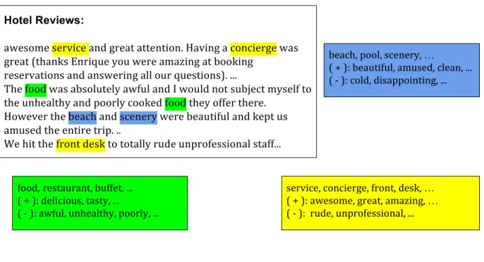
Here in Figure 2.1 we show an example about how word distributions of different senti-ment polarities vary for different topics.

Figure 2.1: Example of topics and sentiment polarities in hotel reviews

There are several other advantages of our model. First and foremost is that it enables us to infer different word distributions for the same topic, with different sentiment polarities. Thus, from different word distributions for different sentiment polarities, we can isolate descriptive words, positive words, and negative words from the same topic.

Another advantage is that our model makes it possible to infer sentiment distributions for each topic mentioned in the document. This will allow researchers and users to develop a deeper and more detailed sentiment analysis for not only the whole document, but also each different aspect in the document. This would potentially aid them in differentiating the distinct views of an author towards the topic aspects that are reflected within a document.

(31)

2.3

Model Definition

As with the model representation that we described in Chapter 2, we define D={d1, d2, ..., dm}

to be the corpus that we want to analyze, and xj = {xj1, xj2, ...} to be the word array in document dj. We then assume that each word xji is associated with a latent dyadic

topic-sentiment combination label, denoted < θ, l >, where θ is the factor corresponding to the observation variable xji, which is associated with one global topic k, and l is one latent

sentiment label from one predefined sentiment label set L.

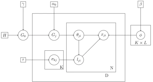
We extend the existing generative model for HDP framework to accommodate sentiment label l for word xji generation as shown in figure 2.2:

H γ G0 α0 Gj θji τ σkj lji xji β φ N D K×L K

Figure 2.2: Plate model for HDP model with sentiment labels

In this model, the global probability measure G0 represents a global topic distribution, drawn from a Dirichlet process with two generative hyperparameters: a base measureH and a concentration parameter γ. Each document j then generates its own probability measure for local topic distribution Gj from a Dirichlet process with G0 as its base measure and α0

(32)

Gj|α0, G0 ∼DP(α0, G0) for each j,

(2.1)

Each observation xji in document j position i has two parameters, θji and lji. θji

is independently and identically distributed (i.i.d.), drawn from Gj. Because each θji is

associated with an observationψjt, which in turn has a corresponding factorkjtsampled from

G0, we can denote θji =ψjt, ψjt =φk where kjt =k. So that eachθji is actually associated

with one global topic group k. In our model, for each distinct k emerged in document

j, we assume that there is a particular sentiment distribution for k denoting the author’s subjective attitude towards this topic. Therefore we generate a Dirichlet distribution σjk

over the sentiment label setL, denoting this sentiment distribution for topic k in document

j, with Dir(τ) as its conjugate prior. Then the sentiment label lji for observation xji is

drawn from this distribution, given its topic label k. This is given by:

σjk ∼Dir(τ) for each existing k in each j,

θji|Gj ∼Gj for each j and i,

lji ∼M ult(σjk_θji) for each j and i,

(2.2)

We want to not only discover the differences of word distributions between same sen-timent polarities in different topics, but also differentiate the word distributions for same topic with different sentiment polarities. Therefore, we assume that each distinct < k, l >

combination should form a distinct word distribution. Here we denote that F(k, l) is a Dirichlet distribution over the whole vocabulary for specific < k, l > combination, which usesDir(β) as its conjugate prior. Then each observationxjiis drawn from this distribution

(33)

F(k, l)∼Dir(β)

xji|θji, lji ∼F(k, l) for each j and i,

(2.3)

To illustrate the generative process of our HDPsent model with sentiment and topic generation, we can extend the generative process of Chinese restaurant franchiseframework for traditional HDP model presented in17 as:

1. Draw an infinite number of topics with predefined set of sentiment polarities: φkl ∼

Dir(β) for k={1,2,3...},L={1,2, ..., l}.

2. Draw stick-breaking topic proportions as νk ∼Beta(1, γ) for k ={1,2,3...}.

(a) we sample document-level topic atoms kjt ∼ M ultinomial(σ(ν)) for each table

t={1,2,3...}.

(b) we then sample document-level stick-breaking proportions as πjt ∼ Beta(1, α)

(c) For each distinct k, we sample the sentiment distribution σjk ∼Dir(τ)

(d) For each token xji in document dj at position i:

i. We sample a latent topic label θji ∼M ultinomial(σ(πj)).

ii. We sample a latent sentiment label lji ∼M ultinomial(σjk_θji)

iii. We sample a word w∼F(θji, lji).

Here σ(ν) and σ(πj) are distributions constructed by stick-breaking algorithm with proportions of ν ={νk|k = 1,2,3, ...} and πj ={πjt|t= 1,2,3, ...}as:

(34)

σk(ν) =νk k−1 Y i=1 (1−νi) σt(πj) =πjt t−1 Y i=1 (1−πji) (2.4)

2.4

Inference

In this section, we want to use the extended Chinese restaurant franchise process (CRFP) generative model that we described above to infer the Gibbs sampling schema for HDPsent

model.

Here we define θ−ji and l−ji are latent labels of all data items except observation xji:

θ−ji :={θj0_i0|j0i0 6=ji}

l−ji :={lj0_i0|j0i0 6=ji}

(2.5)

We assume in this model that each word is drawn from F(< θji, lji >) =φkl, which is

dependent on the combination ofθji andlji. We also assume that the latent sentiment label

lji is drawn from a Dirichlet sentiment distribution for the specific topic parameter factor

θji in document dj. So that we can obtain the posterior conditional of < θji, lji> as:

p(θji, lji|xji,θ−ji,l−ji)

∝p(xji|θji, lji)·p(lji|l−ji,θ−ji, θji)·p(θji|θ−ji)

(2.6)

Here p(θji|θ−ji) denotes the conditional distribution of topic factor θji given all other

data points.

We assume that the topic distribution for observations should follow HDP model; thus, to integrate out G0 and Gj, the conditional distribution calculation for θji in each Gj and

(35)

ψjt for global G0 should be similar to3 equations (24) and (25). These can in turn be represented as follows: θji|θj1, ..., θji−1, α0, G0 ∼ mj· X t=1 njt· i−1 +α0 δψjt+ α0 i−1 +α0 G0 (2.7) and ψjt|ψ11, ..., ψjt−1, γ0, H ∼ K X k=1 m·k m··+γ δφk + γ m··+γ H (2.8)

Now, we designate τk = {τk1, ..., τkL} to represent the probability distribution of

senti-ment label set L for topic k. Since the size of L is predefined, this is a simple multinomial distribution across the document; therefore, we can simply choose a Dirichlet distribution as its conjugate prior:

τk ∼Dir(σ) (2.9)

We assume that each topic existing in one document has its own sentiment distribution. Therefore, the sentiment label for one word in document is independent from other words in this document on different topics. This also follows our intuition in writing a document, our sentiment attitude in different topics would be quite different even in the same document.

Thus, the posterior sentiment distribution of topic k only takes into consideration the counts of word tokens with sentiment labels for the same topic:

p(τk|σ,l,k)∼Dir(σ1+Ndkl1, ..., σL+NdklL) (2.10)

Therefore, the conditional probability of sentiment label lji for each data point xji can

easily obtained by integrating τk out of equation (2.9), given the topic factor θji = φk,

(36)

P(lji|l−ji,k−ji,σ, kxji =k) = Z τlDir(τ|σ1+N −ji dkl1, ..., σL+N −ji dklL)dτ = σl+N −ji dkl P σ+N_dk−ji_· (2.11)

Finally, with the sampled latent variable combination < θji, lji > associated with data

xji, we can obtain the topic label for tablet associated with θji bykjt =k. The word token

of xji should be drawn from word distribution denoted as F(k, l).

For each word distribution for different topic-sentiment combination, we assume that it is derived from a Dirichlet distribution, with conjugate prior H. Here we can simply useφkl

to denote this word distribution. Therefore, the conditional density of xji under < k, l >

can be calculated depending on all data points in the component k possessing the same sentiment label l, leaving xji out; Then we can just directly use3 equation(30) to calculate

the conditional probability of word token variable xji as:

f−xji kl (xji) = p(xji|k, l) = R f(xji|φkl)Qj0i06=ji, θj0i0=k, l_j0_i0=l f(xj0_i0|φ_kl)h(φ_kl)dφ_kl R Q j0i06=ji, θj0i0=k, l_j0_i0=l f(xj0_i0|φ_kl)h(φ_kl)dφ_kl (2.12)

And if the data item xji being assigned to a combination with new topic as< knew, l >,

it means that it is assigned to a newφwith no prior data items. So the posterior probability is only dependent on conjugate prior H, which can be represented as:

f−xji

knew_l(xji) =p(xji) = Z

(37)

2.5

Sampling schema

Using all these probabilities that we derived above, we can now work out the Gibbs sampling schema for posterior sampling of each data item xji using this extended Chinese restaurant

franchise process framework (CRFP) for our HDPsent model.

Sampling t

We denote local index variable for each θji astji, and sample this index variable directly

using Gibbs Sampling and the marginal represented in equation 2.7:

p(tji =t, lji =l|t−ji,l−jik) ∝        n−_jtji·p(lxji|k,l −ji_,_k−ji₎_·_f−xji kjtl (xji) if t previously used, α0·p(xji|t−ji,l−ji,k, tji =tnew) if t is new. (2.14)

For the new table sampled, we can similarly derive the probability as:

p(kjtnew =k, l_ji =l|t,l−ji,k−jt new ) ∝        m·k·p(lxji|k,l −ji_,_k−ji₎_·_f−xji kl (xji) if k previously used, γ·p(lxji|k new_,_l−ji_,_k−ji₎_·_f−xji knew_l(xji) if k is new. (2.15) Here f−xji kl (xji) and f −xji

knew_l(xji) are conditional densities of data xji given all other data

items that can be calculated by equation 2.12 and 2.13.

Sampling k

Similarly, we denote global topic index variable for each ψjt askjt, and sample this index

variable directly.

(38)

it is possible that the data points being assigned to same table share the same topic label

k, but admit different sentiment labelsl.

As a consequence, the data points in the same table may belong to different F(k, l) components. Here we assume that when we sample global topic k for each table, we do not change the sentiment labels of word tokens in this table. So that the probability of one table belongs to a specific k is a combination of probabilities of independent groups of tokens from differentF(k, l) components for all existingl in this table. This probability can be written as: f_k−xjt(xjt) = Y l∈L xjlt={xji|xji∈t,lji=l} p(l|k, d)f_kl−xjlt(xjlt) (2.16)

where P(l|k, d) can be calculated using the posterior probability of the Dirichlet senti-ment distribution that we illustrated in equation 2.11.

And also the probability of one table belongs to a new topicknewshould also be calculated

as a combination of probabilities of these tokens from separate F(knew, l) components for

all existing l in this table. Similarly, this probability can be written as:

f_k−newxjt(xjt) =

Y

l∈L

xjlt={xji|xji∈t,lji=l}

p(l|d)f_k−newxjlt_l(xjlt) (2.17)

Here p(l|d) represents the overall sentiment distribution across the document. Since we have figured out the calculation of f_k−xjt(xjt) and f

−xjt

knew(xjt), the probability of

table t is assigned to each k follows the traditional sampling schema according to2.8 as:

p(kjt =k|t,l−ji,k−jt)∝        m·k·f −xjt k (xjt) if k previously used, γ·f_k−newxjt(xjt) if k is new. (2.18)

(39)

Algorithm 1 HDPsent algorithm

1: procedure _{Gibbs–HDPsent}

2: for each documentdj ∈D do

3: for each word token xji ∈dj do

4: Incrementally sample < θji, lji > forxji

5: Changelji to its predefined inital value lw given word w=xji

6: Increase statistical counts for < θji, lw >

7: end for

8: end for

9: while not converged do

10: for each document dj ∈D do

11: for each word token xji ∈dj do

12: Decrease statistical counts for old < θji, lji >

13: Sample < θ, l > for xji

14: Increase statistical counts for new < θji, lji >

15: end for

16: for each table ψjt ∈dj do

17: Decrease statistical counts for old kjt

18: Sample k for ψjt

19: Increase statistical counts for new kjt

20: end for

21: end for

22: end while 23: end procedure

(40)

2.6

Model Prior

Traditional HDP model rarely introduce asymmetric priors for both documents and topics. However, our model imports aspect-level sentiment layer into traditional HDP model, which requires certain degree of structured asymmetric priors for sentiment modeling.

2.6.1

Sentiment Prior

In our model, the sentiment distribution is dependent only on the data in same topic. This does not cause problems in LDA models, butdoescause problems in HDP models, because HDP model spawns new topics at certain probabilities:

p(τ|σ,l−ji,k−ji, knew)∼Dir(σ1+ 0, ..., σL+ 0) =Dir(σ) (2.19)

Without any prior knowledge for sentiment labels for tokens assigned to new topic (or newly emerged topic with only few tokens assigned to within this document), the sentiment label for this token, is solely (or largely) dependent on its conjugate prior Dir(σ). This is still acceptable if we assume that sentiment distributions of different topics are totally independent from each other in the same document. However, most of the time, we intend to have similar sentiment attitude across most topics we write about in the same document. So that we can set up document-specific priors for sentiment distribution, and topic can have its own sentiment distributions drawn from this prior.

Here we introduce different σ for different documents as its own conjugate prior. Using the LDA prior schema from35 for sentiment distributions, we use σ0 as a concentration parameter for σ, and obtain:

σdl = X l σl· Nd·l+σl0 Nd··+P_lσ0_l (2.20)

(41)

P(lxji|l −ji_,_k−ji_,_σ_{, k} xji =k) =        σdl+N_dkl−ji P lσdl+N −ji dk· if k previously used, σdl P lσdl if k is new. (2.21)

2.6.2

Word Prior

Since our word distribution F(k, l) has only the global conjugate prior Dir(β), as shown in figure 2.2, any new < k, l > combination has the same symmetric prior. In pure topic models, this is acceptable since we do not have and may not set up any prior knowledge for word distribution in the new topic at all. However, on the one hand, we already have strong prior bias for sentiment polarity of many words in English vocabulary, according to their semantic meanings. On the other hand, the sentiment polarity of same word across different topics although is not fixed, but has less tendency to be changed. For example, even though we do not have a prior preference for a word such as ”good” in a new topic knew_{, we shall}

have some prior preference for ”good” in a new combination < knew_{, positive >}_{, versus a}

new combination < knew_{, negative >}_.

This prior also helps us to adjust the probability for sampling word for sentiment labels. Without this prior, the sentiment assignment for words in the same topic can easily be reversed from their usual meaning, with positive words assigned to the predefined negative category, and negative ones to the positive category.

Using the same prior schema, and defining β0 to be the concentration parameter for β, we directly obtain: βlw = X w βw· N·lw+βw0 N·l·+P_wβw0 (2.22)

(42)

f−xji kl (xji) =        βlw+N_klw−xji P wβlw+N −_xji kl· if k previously used, βlw P wβlw = N·lw+βw0 N·l·+Pwβlw0 if k is new. (2.23)

(43)

Chapter 3

Author-Topic Model:

HDPauthor

While the characterization of topic modeling as estimating the topic distribution of doc-uments was developed many years and has been used since, there is also a growing need for topic interest learning of authors. Moreover, the contribution of different authors to a single document is also a learning problem that needs to be studied. Our objective as discussed in this chapter to develop a generative mixture model extending current topic models, which is capable of simultaneously learning and identifying the topic interests of authors, topic distribution across documents, and author contributions to documents.

Currently there are already many significant works on Bayesian methods for author mixture models36 37 _without _{topic modeling. There is also some work in the literature on}

LDA-based author-topic learning frameworks38 39_{. However, because these models are}

vari-ation and extension based on LDA, using Dirichlet multinomial mixture models, all of them admit predefined limits on the number of topics.

In real-world applications, the number global topics across whole corpora may not be fixed or boundable. However, each author usually only works on and is good at a small set of topics, and each document written by a group of authors is also usually written on a small set of topics. Therefore, the nonparametric Bayesian feature of hierarchical Dirichlet process for topic modeling can help us to solve the problem, and infer a better learning

(44)

algorithm compared to existing LDA-based author-topic learning models.

In this chapter, we present a statistical generative mixture model called HDPauthor, for scientific articles with authors; this model extends our existing HDP model to incorporate authorship information. It uses nonparametric hierarchical Bayesian modeling to learn the topic interests of each author across the documents in which that author participates. It treats the topic distribution for local multi-author document as a finite mixture of distri-butions of the authors. It benefits from traditional HDP model features that the global number of topics is unbounded. Each author from text collection also shares unbounded number of topics from global topic pool. This model also enables researchers and users to infer contribution proportions of different authors for one document.

3.1

Related Work

There are many works that have already incorporated co-authorship into topic modeling. One significant model is the Author-Topic model38 40. This model extends the LDA model to include authorship information. It makes it possible to simultaneously learn both the relevance of different global topics in document, and the interests of topics for authors. It associates not only a mixture of topics with each document but also a mixture of topics with each author, which makes it able to sample words from probability distributions generated usng a combination of these two factors. In similar fashion to the LDA model, the total number of topics for the whole corpus must be predetermined in advance, with no flexibility over the number of topics generated. This model also lacks the ability to share only a small subset of topics across different documents, as well as across different authors. Therefore, it learns distribution of each topic in this large group of topics for each document and each author.

Models proposed by Dai41 42 are based on nonparametric HDP model for topic-author problem. This approach combines author identities with associated topics as a group. This

(45)

group defines a Dirichlet process (DP) over author entities and topics, which in turn is then drawn from a global author and topic DP. This model is mainly geared towards disambigua-tion of author entities. However, this model combines authors and topics in the same DP, which fails to decouple topics from authors. Therefore, it lacks the ability to share the same topics between different authors, and also makes it difficult to infer author contributions to these documents.

3.2

Model Introduction

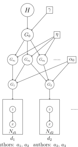
Our HDPauthor model is a nonparamatric hierarchical Bayesian model for author-topic generation. This model assumes that topic distribution of each document is a finite mixture of distribution components of the authors of this document. We can then infer that each token in the document is written by one and only one of the authors in the author list of this document, associated with the topic distribution of this author. This assumption enables us to set up latent author label for each word token along with its topic label. This latent author label helps us to infer both topic interests of authors and mixture parameters in documents for each author.

By using an HDP framework, we also assume that each author is associated with a topic distribution which is drawn based on the same underlying base measure as global topic distribution in whole corpora, with different variability. The global topic atoms are shared by all authors, but each author only occupies a small subset of these global topic components, with different stick-breaking weights. This local probability measure of each author represents the topic interests of this author. Different authors share different topic interests.

The topic distribution of each author is learned using the mixture generative model of all documents that the author participates in. The topic distribution of each document is not drawn from the global topic distribution directly, but represented by this mixture model

(46)

of all its authors indirectly. Since we already assume that each token is written by one and only one of the authors with the particular topic distribution of this author, then the latent topic labels combined with latent author labels helps us to infer the topic distribution of documents. Therefore, each document is represented by a union of all topics contributed by each of its authors.

Here in Figure 3.1 we illustrate an example of document produced through the coop-eration of several authors. The content of the document is the abstract of one paper43 _on

machine learning for gene expression data. AuthorYoseph Barash mainly works on biology and bioinformatics, who contributes more on biology related topics, while authorNir Fried-man is an expert in Bayesian inference and machine learning, which results in his having higher probability of machine learning-related topics.

(47)

3.3

Model Definition

The document representation in our model also follows our definition stated in Chapter 2. We assume D = {d1, d2, ...} is a collection of scientific articles, composed of a series of words from vocabulary V as xj ={xj1, xj2, ....}. Furthermore, in ourHDPauthor model, we have extra co-authorship information. We assume that each document has a set of authors

aj ={aj1, aj2, ...} who cooperated in writing this document dj.

Previously we have assumed that each token in a document is written by one of the authors for this whole document. Therefore, here we associate one latent author label q

from the author set aj for each token in documentdj along with original latent topic label

k.

This latent author labela not only helps us to directly calculate the contribution of each author for the document, but also enables the aggregation of topic distribution for each author across the whole corpus.

We generate G0 as the corpus-level set of topics as a Dirichlet Process with H as base measure and γ as its concentration parameter. A topic component is denoted φg. Each

author a that exists in the entire corpus corresponds to a Dirichlet Process Ga that shares

the same global base distribution of topics G0, with concentration parameter η. As with the HDP model, the author-level Ga only shares a small subset of corpus-level topics.

Ga|η, G0 ∼DP(η, G0)

(3.1)

Unlike in the traditional HDP model, we do not draw a Dirichlet process Gj of each

document dj from the global G0 as Gj ∼ DP(α0, G0). Instead, we set up a mixture of components from probability measures of all authors of this document. We then denote the mixing proportion vector as πj =< πj1, ..., πj|aj| >. Therefore, all of its elements must

(48)

be positive and sum to one. Since each document is written by a fixed group of authors, we can here simply assume that πj is drawn from a symmetric Dirichlet distribution with concentration parameter .

πj ∼Dir() (3.2)

For a mixing proportion vector πj, there are two ways of drawing Gj from a Dirichlet

process for the mixture of the probability measures of all its authors, designated{Ga|a∈aj}.

The first method is to combine the probability measuresGaof authors as a new base measure

first, then draw a DP with this base measure combination for document dj; this DP can be

formulated as follows:

Gj ∼DP(α0,

X

a∈aj

πja·Ga) (3.3)

Another method is to first draw separate DPs from each of the authors of the document

dj with the author’s own probability measure Ga as the base measure, and then calculate

the probability measure of dj as a mixture of these DPs. The mathematical formula we

derive for this method is:

Gj ∼ X

a∈aj

πja·DP(α0, Ga) (3.4)

Each observation xji in documentdj is associated with a combination of two parameters

< aji, θji > sampled from this mixture Gj. In this combination, aji is author label a ∈aj,

which indicates the ”class” label of this author mixture model. θjiis the parameter specifying

the one of the author’s topic component for xji, which is sampled from the probability

measure Ga of the author a selected. Therefore, this θji is associated with table tji, which

is an instance of mixture component ωak from author a = aji; ωak is then associated with

(49)

component factor assigned to kjt in its associated parameter θji, denoted asF(g):

< aji, θji >|Gj ∼Gj

xji|θji ∼F(θji)

(3.5)

As we explained above, the factor θji for each observation xji is associated with global

topic mixture component g. Here we can simply use φg to denote this distribution.

There-fore, the conditional density of each observation xji under this particularφg given all other

observations can be derived similarly to3 _{equation(30):}

f_g−xji(xji) = R f(xji|φg) Q j0i06=ji, θ_j0_i0=g f(xj0_i0|φ_g)h(φ_g)dφ_g R Q j0i06=ji, θ_j0_i0=g f(xj0_i0|φ_g)h(φ_g)dφ_g (3.6)

And the conditional probability of data item xji being assigned to a new topic gnew is

also only dependent on the conjugate prior H. This can be represented as:

f_g−newxji(x_ji) =

Z

f(xji|φg)h(φg)dφg (3.7)

Here in figure 3.2 we illustrate the graphical plate model for ourHDPauthor model with one more layer of author probability measures injected into the original HDP model:

To present the generative process of ourHDPauthormodel within an author layer, we can extend the generative process of Chinese restaurant franchise framework for the traditional HDP model presented in17 _as:

1. Draw an infinite number of topics φg ∼Dir(β) for g ={1,2,3...}.

2. Draw stick-breaking topic proportions as νg ∼Beta(1, γ) forg ={1,2,3...}.

(50)

H

γ G0 Ga1 Ga2 Ga3 ... η α0 G1 z x Nd1 d1 authors: a1, a2 G2 z x Nd2 d2 authors: a2, a3 ...

Figure 3.2: Plate Model for HDP model with authors

(a) we sample author-level topic atoms gak ∼ M ultinomial(σ(ν)) for each author

componentka={1,2,3...}.

(b) we then sample author-level stick-breaking proportions as µak ∼ Beta(1, η) for

each author component ka={1,2,3...}.

(a) We sample the author mixing proportions for authors of this document as πj ∼

Dir()

(b) we sample document-level author component atoms kjt from the author mixture

(51)

(c) We then sample document-level stick-breaking proportions as δjt ∼ Beta(1, α)

(d) For each token xji in document dj at position i:

i. We sample a latent topic label θji ∼M ultinomial(σ(δj)).

ii. We sample a word w∼M ultinomial(φθji).

Here σ(ν) and σ(δj) are distributions constructed by stick-breaking algorithm with proportions of ν ={νk|k = 1,2,3, ...} and δj ={δjt|t= 1,2,3, ...}as:

σk(ν) =νk k−1 Y i=1 (1−νi) σt(δj) =δjt t−1 Y i=1 (1−δji) (3.8)

3.4

Inference

The primary inferential mechanism for our model is based on a Gibbs sampling-based imple-mentation of the Chinese restaurant franchise process (CRFP) model. We should extend this representation framework to inject an author layer, and calculate all posterior distributions for latent variables.

Inference for model (3.3)

Here we compute the marginal of Gj under this author mixture Dirichlet process model

with G0 and Ga are integrated out. We want to compute the conditional distribution ofθji

given all other variables; we thus extend3 equation (24) to fit our model for model 3.3, to obtain: θji|θj1, ..., θji−1, α0, Gj, Ga0, Ga1, ...∼ mj· X t=1 njt n−_j_·ji+α0 δψjt + α0 n−_j_·ji+α0 X a∈aj πja·Ga (3.9)

(52)

Here, ψjt represents the table-specific indicator that indicates the component choice kjt

from author ajt’s probability measure. A drawing from this mixture model can be divided

into two parts. If the former summation is chosen, then xji is assigned to an existing

ψjt, and we can denote θji = ψjt. If the latter summation is chosen, we have to create a

new document-specific table tnew_{, and assign it to one of the authors according to mixing}

proportion vector of authors for documentdj, where eachπja∈πj represents the probability that table tnew _{belongs to author} _a_{. Then we can draw one new}_ψ

jtnew from the probability measure of author a represented as Ga.

Ga for each author a in the corpus appears in all documents in which this author

par-ticipates. It should be integrated out through all ψjt that ajt =a. We use mak to indicate

the total number of tables t such that kjt = k and ajt = a. To integrate out each Ga, we

can get: ψjt|ψ11, ..., ψjt−1, η, G0 ∼ la·· X k=1 mak ma··+η δωak + η ma··+η G0 (3.10)

This mixture is also divided into two parts. If we draw sample ψjt from the former part,

then we assign it to an existing component k from authora, we can denote it asψjt =ωak.

If the latter part is chosen, we will create one new component knew for author a. and we

draw this new ωaknew from global topic probability measure G0.

Finally we can integrate out this global probability measureG0 by all cluster components

ωak from all existing authors in whole corpora. Here we uselg to indicate the total number

of ωak such that gak =g. The integral can then be represented similarly to3 equation (25):

ωak|ω11, ..., ωak−1, γ, H ∼ G X g=1 lg· l··+γ δφg + γ l··+γ H (3.11)

Similarly, if the former is chosen, we assign the existing topic component φg to ωak; if

the latter is chosen, we create a new topic gnew _{sampled from base measure} _H_.

(53)

For mixing model 3.4, each document’s probability measure is divided into |aj|

inde-pendent components, where the probability of each component a ∈ aj to be chosen is

determined by πja ∈ πj from this document-specific mixing proportion vector πj. Once a

specific author a is chosen, the probability distribution of θji follows the Dirichlet process

DP(α0, Ga) where a ∈ aj, using the probability measure of author a denoted as Ga to be

its base measure. Therefore, withG0 andGa integrated out, we can obtain the distribution

of θji given all other variables, as:

θji|θj1, ..., θji−1, α0, Gj, Ga1, Ga2, ...∼ X a∈aj πja· mja· X t=1 njt n−_jaji_· +α0 δψjt+ α0 n−_jaji_· +α0 Ga (3.12)

These two models differ only in the construction of the mixture of authors with each author’s own probability measure, drawn from shared global infinite topic mixture model in one document. The constructions of each author’s probability measure and global topic measure are same. Therefore, the posterior conditional calculation of ψjt andωak for model

(3.4) are same as presented in equation 3.10 and 3.10.

3.5

Sampling schema

According to this series of marginals that we integrated out above, we can now go on to calculate the posterior sampling schema for our Gibbs sampling inference process.

Since we have two mixture models for combining author topic components into one document, as stated in mixture model (3.3) and model (3.4), the integrals that we inferred in equation3.9and equation3.12will result in two different ways of calculating the posterior conditional distributions of aji and θji accordingly.

(54)

3.5.1

Sampling schema for author mixture model (

3.3

)

Sampling t

Using the integral 3.9 inferred for author mixture model (3.3), the probability that tji

takes a particular existingtshould be proportional to the number of tokens in thistasn−_jtji, regardless of the author label ajt for this table t, and the probability that this xji will be

assigned to a new value t is proportional to α0.

p(tji =t|t−ji,a,k,g)∝        n−_jtji n−_j·ji+α0 ·f −xji

g_akjt(xji) if t previously used,

α0

n−_j_·ji+α0

·p(xji|tji =tnew,a,k,g) if t is new.

(3.13)

If the sampledtjiis newt, we should then sample the author labelajt for this tabletfrom

the Dirichlet-based finite author mixture model, and then sample k from the probability measure of author a, given ajt =a:

p(kjtnew =k, a_jtnew =a|t−ji,a−jt new ,k−jtnew,g) =p(ajtnew =a|a−jt new )·p(kjtnew =k|a_jtnew =a,t−ji,k−jt new ,g) (3.14)

We already denote the mixing proportion vector of authors for document dj by πj.

We also assume that this vector follows a Dirichlet distribution with as its conjugate prior. However, since in this model, we use tabletas the base granularity for author-mixing representation, we should use the number of tablesmrather than the number of tokensnfor this finite author mixing proportion calculation. Here we use mja to represent the number

of tables assigned to author a in document dj. Thus, we can use the standard Dirichlet

integral to calculate posterior probability of author labelajt for this document-specific table

(55)

p(ajt =a|a−jt, ) =

m−_jajt + m−_j_·jt+|aj| ·

(3.15) With the author label ajtnew = a selected, we already