Improving interpretability and regularization in deep learning

White Rose Research Online URL for this paper:

http://eprints.whiterose.ac.uk/150521/

Version: Accepted Version

Article:

Wu, C., Gales, M.J.F., Ragni, A. et al. (2 more authors) (2018) Improving interpretability

and regularization in deep learning. IEEE/ACM Transactions on Audio, Speech, and

Language Processing, 26 (2). pp. 256-265. ISSN 2329-9290

https://doi.org/10.1109/taslp.2017.2774919

© 2017 IEEE. Personal use of this material is permitted. Permission from IEEE must be

obtained for all other users, including reprinting/ republishing this material for advertising or

promotional purposes, creating new collective works for resale or redistribution to servers

or lists, or reuse of any copyrighted components of this work in other works. Reproduced

in accordance with the publisher's self-archiving policy.

[email protected] https://eprints.whiterose.ac.uk/

Reuse

Items deposited in White Rose Research Online are protected by copyright, with all rights reserved unless indicated otherwise. They may be downloaded and/or printed for private study, or other acts as permitted by national copyright laws. The publisher or other rights holders may allow further reproduction and re-use of the full text version. This is indicated by the licence information on the White Rose Research Online record for the item.

Takedown

If you consider content in White Rose Research Online to be in breach of UK law, please notify us by

Improving Interpretability and Regularisation in

Deep Learning

Chunyang Wu

, Mark Gales

, Anton Ragni

, Penny Karanasou

and Khe Chai Sim

Department of Engineering, University of Cambridge, Trumpington Street, Cambridge CB2 1PZ, UK

2

Google Inc., Mountain View, USA

Abstract—Deep learning approaches yield state-of-the-art per-formance in a range of tasks, including automatic speech recognition. However, the highly distributed representation in a deep neural network (DNN) or other network variations is difficult to analyse, making further parameter interpretation and regularisation challenging. This paper presents a regularisation scheme acting on the activation function output to improve the network interpretability and regularisation. The proposed approach, referred to as activation regularisation, encourages activation function outputs to satisfy a target pattern. By defining appropriate target patterns, different learning concepts can be imposed on the network. This method can aid network interpretability and also has the potential to reduce over-fitting. The scheme is evaluated on several continuous speech recognition tasks: the Wall Street Journal continuous speech recognition task, eight conversational telephone speech tasks from the IARPA Babel program and a U.S. English broadcast news task. On all the tasks, the activation regularisation achieved consistent performance gains over the standard DNN baselines.

Index Terms—activation regularisation, interpretability, visu-alisation, neural network, deep learning

I. INTRODUCTION

Recent progress in deep learning [3], [4], [5] has improved the state-of-the-art performance in a range of applications, including the automatic speech recognition (ASR) systems. The multiple layers of non-linear transformations in a deep neural network (DNN), or related network variations, allow complex and difficult data to be well modelled. However, its high-level abstraction and representation of input features make it difficult to interpret the DNN parameters. This can cause various issues for improving parameter estimation, and network generalisation.

To reduce over-fitting, regularisation techniques are com-monly used in DNN training. Weight decay adds a squared L2-norm term of the DNN parameters to the cost function. This penalises large weights during parameter optimisation. Rather than modifying the criterion, dropout [6] randomly The research leading to these results was supported by the Intelligence Advanced Research Projects Activity (IARPA) via Department of Defense U.S. Army Research Laboratory (DoD/ARL) contract number W911NF-12-C-0012; Singapore Ministry of Education Academic Research Fund Tier 2 (Official Project No: MOE2014-T2-1-068); research projects and donations from Google and Amazon. The U.S. Government is authorized to reproduce and distribute reprints for Governmental purposes notwithstanding any copy-right annotation thereon. Disclaimer: The views and conclusions contained herein are those of the authors and should not be interpreted as necessarily representing the official policies or endorsements, either expressed or implied, of IARPA, DoD/ARL, or the U.S. Government.

This work is an extension of its conference version presented in [1], [2].

turns off, drops, a set of nodes during the training procedure; as a result, the final DNN can be viewed as an ensemble model of many small DNNs. This averaging helps reduce over-fitting to the training data. Optimisation techniques, such as batch normalisation [7], can also be used to accelerate the training and obtain a better generalised performance. However, these approaches do not aid the interpretability of network parameters. Structured neural networks introduce interpretation by adding structure to the network topology. Different groups of parameters, or nodes, are introduced and restricted to model specific aspects of the data. Inspired by the animal visual cortex, convolutional neural networks [8], [9] (CNNs) introduce convolutional, pooling, and fully-connected layers to restrict the network connectivity. Multi-task neural networks [10], [11], [12] change the output layer with auxiliary tasks to further reinforce the primary task. Mixture density networks [13], [14], [15] parametrise the mixture components via DNNs, effectively modelling a “deep” probability density function. Multi-basis adaptive neural networks [16], [17] in-volve parallel sub-networks to cover different data domains.

A number of approaches have been proposed to interpret trained DNN parameters. Reverse engineering methods have been investigated to analyse the hidden unit representations. These schemes focus on analysing a well-trained neural net-work, instead of inducing useful interpretations during the training process. For instance, Garson’s algorithm in [18], [19] was used to inspect feature importance in DNN models. In the area of computer vision, weight analysis of neural networks has been examined to interpret neural networks. In [19], [20], [21], the input feature was optimised to maximise the output of a given hidden activation in the network. The visualisation of the feature implies the function of that ac-tivation. [22] inverted the activations and transformations of convolutional neural networks via the forward propagation step to reconstruct the input features detected by an activation. Alternatively, topographic filter maps [23] impose a spatial order in which the nodes of a CNN are arranged closely on a 2-dimensional (2D) grid. This is implemented by adding a regularisation term to the criterion that reduces the difference of activation function outputs between nearby nodes. Similarly, the mismatches between spatial neighbours can be controlled to smooth activation function outputs for achieving a better regularisation in speaker adaptation [1] or in DNN training [5]. This paper describes a method to both improve inter-pretability and regularisation of DNNs. A general framework is proposed based on this concept, referred to as activation

regularisation. Instead of being treated independently, the nodes in hidden layers are reorganised to form an activation grid. A reference, named as target pattern, is introduced. The target pattern can encode a range of learning concepts, which can induce interpretability. This information is then used as a regularisation term to train the model parameters. By adding a regularisation term to the cost function, activation function outputs can be controlled to satisfy a target pattern in the training phase. In this way, the DNN behaviour can be interpreted by visualising and inspecting the network grid. Also, this regularisation has the potential to reduce over-fitting and improve the capability to generalise DNNs. For the discussion of the framework, this paper focuses on DNNs. However, this approach can be applied to more complex models such as recurrent neural networks.

The rest of this paper is organised as follows. The basic DNN topology and notations are reviewed in Section II. Sec-tion III proposes the framework for activaSec-tion regularisaSec-tion. Experiment results and discussions are reported in Section IV. The conclusion of this paper is presented in Section V.

II. BASICDNN TOPOLOGY

In speech recognition, DNN models are commonly used to predict the context-dependent state emitting probability p(xt|y)at timetvia a pseudo-likelihood

p(xt|y) =

P(y|xt)p(xt) P(y) ∝

P(y|xt)

P(y) (1)

wherextandy, respectively, represent the feature vector of an acoustic observation and a context-dependent state; as p(xt) is independent of y, it can be ignored. This paper takes the feed-forward neural network as an example for the discussion of the proposed method. A feed-forward DNN maps the input feature vectorxtonto a set of output targetsythrough a series of hidden layers. Each hidden layer introduces a number of nodes and an activation function for each node. The activation function inputz(tl) and outputh

(l)

t are recursively defined as

z(tl)=W(l)Th (l−1) t +b(l),1≤l≤L (2) h(tl)=φ zt(l) ,1≤l < L (3) h(0)t =xt (4)

where Ldenotes the total numbers of layers; φ(·)represents the activation function;zt(l)represents a transformation given on the l-th layer; and the parameters of the transformation are defined as W(l) _{and b}(l)_{. DNN models use non-linear}

activation functions to yield highly distributed representations. The activation function φ(·) can take many forms, such as sigmoid function φizt(l) = 1 1 + exp−z(til) ; (5)

hyperbolic tangent (tanh) function φizt(l) =1−exp −2zti(l) 1 + exp−2zti(l) ; (6)

or rectified linear unit (ReLU) function φizt(l)

= max0, z(til)

. (7)

These functions allow the network to derive high-level feature abstractions. At the DNN output, a softmax function is used for multi-label classification tasks. It models the target posterior given the input network representation

P(y=i|xt) = exp z(tiL) P jexp z(tjL) . (8)

In ASR, y commonly stands for the context-dependent state target, which may contain thousands of targets [3].

Letθ=

W(1)_,b(1)_{, . . . ,W}(L)_,b(L)

denote the DNN pa-rameters. Given training data and a suitable criterionL(θ), the parametersθ can be optimised via the error back-propagation algorithm. The cross-entropy (CE) criterion is a standard criterion for frame-wise training

L(θ) =−1 T T X t=1 logP(yt|xt;θ) (9) where T is the total number of training samples; xt and yt are an acoustic feature vector and its context-dependent target, respectively. For sequential tasks such as speech recognition, sequential criteria can also be used. For instance, the minimum phone error (MPE) criterion [24] is defined as

L(θ) =X u X H P(H|Xu;θ)lev(H,Href u ) (10) where u ranges over the training utterances; H represents a hypothesis for that utterance; Xu = [xu1, . . . ,xuTu] denotes

the whole feature sequence with Tu frames belonging to the u-th utterance; and lev(H,Href

u ) represents the Levenshtein distance between the candidate H and the reference Href

u . The tuned, well-trained, DNN is then integrated into an HMM framework to yield the acoustic model in ASR systems.

III. ACTIVATIONREGULARISATION

One issue in neural network training is that the hidden-layer nodes can take an arbitrary order and thus are not inter-pretable. This can cause problems for network regularisation and speaker adaptation as it is difficult to relate parameters to each other. One example is LHUC [25] speaker adaptation where the number of parameters to adapt is equal to the number of nodes. It is difficult to robustly estimate a large number of parameters when there is limited adaptation data.

Activation regularisation encourages outputs of the acti-vation functions to relate to some reference, referred to as the target pattern. By defining appropriate target patterns, meaningful learning concepts can be imposed to influence activation function behaviour. Moreover, appropriately manip-ulating the network nodes into a specific order prevents an arbitrary ordering, which has the potential to improve network regularisation.

The activation regularisation is achieved by adding a regu-larisation termR(θ)to the training criterionF(θ)

whereL(θ)is the standard training criterion; andηdetermines the contribution of the activation regularisation term R(θ). The framework for activation regularisation can be described in four discrete stages:

1) The network nodes in one layer are first rearranged to form a grid, and activation function outputs can then be expressed asHt∗(l).

2) A transformation T(·) is then applied to the activation function outputs, which yields H˜t∗(l).

3) A target pattern G(tl) is specified. Various concepts can be embedded in the target pattern, for example, interpretation or smoothness.

4) GivenH˜t∗(l)andG

(l)

t , a suitable regularisation function

R(·) is applied to minimise the difference between the activation outputs and target pattern.

A. Activation Grid

As discussed in standard network training, nodes of hidden layers can take an arbitrary order. This lack of an ordering constraint leads to two problems: first, a direct visualisation of a layer gives no insights or interpretations; second, manip-ulation of nodes beyond individual elements is challenging.

To introduce a spatial order, an activation grid can be defined for each layer. For instance, a layer with 1024nodes can form a32×322D grid. Given a network with parameters

θ and an input observation xt, the reorganisation operation

G(xt,θ)generates the grid representationHt∗(l)for activation function outputs in each hidden layerh(tl)

G(xt,θ) =hHt∗(1),H ∗(2)

t ,· · ·,H ∗(L−1)

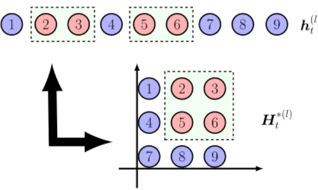
t i. (12) In a 2D space, Ht∗(l) is a matrix; in higher dimensional settings,Ht∗(l)can be described as a higher-order tensor. This paper takes the 2D situation as an example for the discussion. Figure 1 shows an example of a hidden layer with 9 nodes: non-contiguous nodes (in dotted boxes) can form a region in its grid representation. This grid is projected onto a Cartesian

h(tl) Ht∗(l) 1 2 3 4 5 6 7 8 9 1 2 3 4 5 6 7 8 9

Fig. 1. Node Re-organisation to Form a Grid for One Hidden Layer. Non-contiguous elements (in dotted boxes) can form a region in the grid representation.

coordinate system, and each node (i, j) can be located as a point in this network-grid space, denoted as sij.

B. Activation Transformation

Given the activation grid, a transform can then be applied to the outputs of the activation functions. For instance, activation function outputs of the grid can be normalised and transformed to form an activation “distribution”, or a high-pass filtered ac-tivation “image”. The transformed acac-tivation function outputs are defined asH˜t∗(l), specified by a transformT(·)applied to

Ht∗(l)

˜

Ht∗(l)=T(H ∗(l)

t ). (13)

There are multiple possible transformsT(·). A trivial method is the identity transform, which yields the original activation function output

˜

Ht∗(l)=H ∗(l)

t . (14)

Three types of the transforms are investigated in this paper: the normalised activation; the probability mass function; and the high-pass filtering.

1) Normalised Activation: The outputs of the activation functions can directly be used as the transformed represen-tation. However, this may cause a problem since some of the activation function outputs only stay close to the extreme ends of the range of activation function. At the same time, the contribution that they make to the next layer also depends on the parameters of the following layer. Therefore, both the output range of an activation function and its associated parameters to the next layer should be considered as impact factors. Thenormalised activation[26] is proposed to address these problems. It is defined as

˜ h∗tij(l)=h ∗(l) tij β (l) ij (15)

where the termβij(l)is introduced to reflect the impact that the activation has on the following layerl+ 1

β(ijl)=

s X

k

w(kil+1)2o . (16)

where io _{represents the original node index in h}(l) t of the (i, j)-th grid node. This form gives a method to take into account both aspects of the problem: the empirical range of the activation function, and the influence of the next-layer parameters.

The normalised activation can be integrated with other ap-proaches of transformation,e.g., the probability mass function or the high-pass filtering presented as follows.

2) Probability Mass Function: This grid can also be treated as a discrete probability space. By transforming activation function, a probability mass function (PMF) can be obtained that contains information about the activation function be-haviour. This probability mass function can be defined as follows ˜ h∗tij(l)= h∗tij(l) P m,nh ∗(l) tmn (17) where activation function outputs are normalised by their sum. By using this artificial distribution, activation outputs are normalised in a similar range. This normalisation overcomes the potential impact of different activation function types.

There are some constraints that need to be satisfied for this PMF transform. To ensure that H˜t∗(l)is a valid distribu-tion, ˜h∗tij(l) should be non-negative. This restricts the potential choices of activation function. Simple methods such as an exp(·) wrapping can be utilised for an arbitrary function, but this may disable the effect of the negative range in the activation function.

3) High-pass Filtering: A high-pass filtering transform can be used to induce smoothness over the activation function outputs. It includes information about nearby units via a convolution operation,

˜

Ht∗(l)=H ∗(l)

t ∗K (18)

where K is a filter. The filter can take a range of forms. a Gaussian high-pass filter, used in [1], assigns the impact of other nodes according to the distance; a simple3×3 kernel, used in [5], only introduces adjacent nodes.

Using this high-pass filter, the transformation incorporates information from the nearby nodes. For example, by encour-agingH˜t∗(l)to be zero, nearby nodes in the grid space would have similar behaviours. It also yields a smooth surface on the grid, and nearby nodes tend to activate simultaneously.

C. Target Pattern

Activation regularisation encourages the transformed acti-vation function output H˜t∗(l) to satisfy a target patternG

(l)

t . The target pattern can encode a range of learning concepts, which can induce interpretability. Two types of target pattern can be used: a time-variantpattern defines target patternG(tl) depending on the data; and a time-invariant pattern controls the behaviour ofH˜t∗(l)with a static pattern G(l).

1) Time-variant Patterns: The activation grid can be split into a set of spatial regions. The meanings of regions can take a variety of concepts,e.g., phones, noise types or speaker variations. In this way, different grid regions can model and respond to different concepts in the data.

For example, phone-dependent patterns encourage the grid regions to model different phones. In each hidden layer, a set of phoneme (or grapheme) dependent target patterns is defined over the grid. Effectively, a point in this grid space is associated with each phone /p/, denoted as sp. These phone positions can be determined via methods such as t-SNE [27] using the acoustic feature means of the phones. It is then possible to apply a transform to target patterns, in a similar fashion to its activation function output transform

gtij(l)= exp −₂1_σ2||sij−sˆpt|| 2 2 P m,nexp −2σ12||smn−sˆpt|| 2 2 (19)

where sˆpt is the position in the grid space of the “correct”

phone at time t; and σ controls the sharpness of the surface of the pattern. For each phone, a Gaussian contour is defined at its nearby region in the grid. It encourages nodes to correspond to the same phone to be grouped in the same area.

2) Time-invariant Patterns: Time variant patterns require the concept of several “labels” to be derived from the data. This is not necessary. Time invariant patterns can be used to specify general, desirable, attributes of the network activation pattern. It can be expressed as

G(tl)=G(

l)_{,∀t. (20)}

For example, by using a zero pattern,

G(tl)=0, (21)

transformed activation outputs are penalised to have small values, which is similar to the standard L2 regularisation. D. Regularisation Function

A functionR(θ)is now required to relate the transformed activation outputH˜t∗(l) and target pattern G

(l) t R(θ) = 1 T X t X l D( ˜Ht∗(l),G (l) t ) (22) where D( ˜Ht∗(l),G (l)

t ) measures the mismatch between the activation output and the target pattern. There are a range of approaches to defining the difference D(·,·). Three are investigated in this paper: the mean squared error; the KL-divergence; and the cosine similarity. They can all be inte-grated into the error back-propagation algorithm by simply changing the gradient calculation accordingly.

1) Mean Squared Error: A straightforward way to define the difference is the mean squared error method, defined as

D( ˜Ht∗(l),G (l) t ) =||H˜ ∗(l) t −G (l) t ||2F (23) where||A||F stands for the Frobenius norm of a matrix

||A||F = s X i,j a2 ij. (24)

This regularisation method minimises the element-wise squared error between H˜t(l) andG

(l)

t . As an example, using the raw activation function output as the transformed one and setting a time-invariant target pattern G(tl)=0, yields

D( ˜Ht∗(l),G

(l)

t ) =||H ∗(l)

t ||2F. (25) This is similar to standard L2-norm regularisation, but is applied to activation function outputs rather than the parame-ters. Alternatively using a high-pass filtering and a zero time-invariant target patternG(tl)=0yields

D( ˜Ht∗(l),G

(l)

t ) =||H ∗(l)

t ∗K||2F. (26) The output of an activation function is encouraged to be smoothed to its nearby ones; thus a smooth surface is formed in a local region of the grid [5].

The mean squared error regularisation works well when the elements in H˜t∗(l) andG

(l)

t are in a similar range. However, this may require careful selection of the target patterns de-pending on the activation function. For activation functions with fixed ranges, such as sigmoid or tanh, G(tl) can be easily rescaled to an appropriate range. However, for activation functions such as ReLU, in which the range is not restricted, the rescaling onG(tl)tends to require a lot of empirical trials.

2) KL-Divergence: One way to address the dynamic range issue between H˜t∗(l) and G

(l)

t is to use the PMF normali-sation, combined with distribution distances such as the KL-divergence method. The differenceD( ˜Ht∗(l),G

(l)

t )is the KL-divergence of the two distributions [1], the target pattern Gt and the activation distribution H˜t∗(l),

D( ˜Ht∗(l),G (l) t ) = X i,j gtij(l)log gtij(l) ˜ h∗tij(l) ! . (27) For example, by using the phone-dependent target pattern (Eq. 19) and the probability mass function (Eq. 17), the KL-divergence can spur different regions in the grid to correspond to different phones.

3) Cosine Similarity: The KL-divergence regularisation re-quiresH˜∗(l)_{to be positive, to yield a valid distribution. This}

limits the choices of activation function. There are approaches to convert specific activation functions to be positive. For example, by using tanh +1, instead of tanh, in Eq. 17, the KL-divergence regularisation can manipulate the hyperbolic tangent function with a similar pattern as a sigmoid one. However, these methods require a pre-defined lower-bound on the activation function, which cannot be applied in all cases. An alternative approach, the negative cosine similarity, can be used D( ˜Ht∗(l),G (l) t ) =−cos vec_H˜_t∗(l)_,vec_G(_tl) =− P i,j˜h ∗(l) tij g (l) tij H˜ ∗(l) t _F G (l) t _F (28)

where vec_{(·) converts a matrix to a vector representation.} This regularisation defines the similarity between two vectors in an inner-product space. It measures the difference as the angle between the activation output vector vec

˜

Ht∗(l)

and the target pattern onevec

G(tl)

. This supports all forms of activation function.

IV. EXPERIMENTS

Experiments were conducted on three tasks: the Wall Street Journal (WSJ) continuous speech recognition task [28]; eight conversational telephone speech tasks from the IARPA Babel program [29]; and the U.S. English broadcast news (BN) task [30], [31]. The GMMs, DNNs and proposed models were trained on a modified version of HTK Toolkit 3.5 [32].

Three types of activation regularisation were investigated in these experiments:

1) KL: The KL system used the KL-divergence regularisa-tion (Eq. 27) with the activaregularisa-tion PMF (Eq. 17) and the phone-dependent target pattern (Eq. 19). The activation grid of this DNN was encouraged to have phone regions. 2) Cos: The Cos system used the cosine similarity regular-isation (Eq. 28) with the normalised activation (Eq. 15) and the phone-dependent target pattern (Eq. 19). This activation grid was encouraged to have phone regions, which was similar to the KL system.

3) Smooth: The smooth system used the mean-squared-error regularisation (Eq. 23) with the high-pass filtering

activation transformation (Eq. 18) and the zero target pattern (Eq. 21). A 3×3 kernel was used as the high-pass filter, in which the central tap was 1 and others were -0.125. In this way, the activation function outputs were smoothed with their adjacent ones in the grid; and a smooth surface was formed over the activation grid. A. Wall Street Journal

In this task, systems were trained on the 15-hour Wall Street Journal training set (WSJ-SI84) from 84 speakers and evaluated on both the 1994H1-Dev andH1-Eval testsets. Decoding was performed with the WSJ tri-gram language model.

First, the 39-dimensional PLP+∆+∆∆ processed by both global cepstral mean normalisation (CMN) and cepstral vari-ance normalisation (CVN) were used to train a GMM-HMM model (with about 3k tied triphone states). This GMM system was then used to obtain the state-level alignment of the training set for the DNN systems. The 468-dimensional DNN input feature was the PLP+∆+∆∆+∆∆∆ (both processed by global CMN and CVN) in a temporal context window of 9 frames. Three activation functions were used for DNNs: sigmoid, tanh and ReLU. For each one, the respective DNN consisted of 5 hidden layers with 1024 nodes in each layer. Its parameters were initialised in the layer-wise discriminative pre-training setting and then optimised by back-propagation on the cross-entropy criterion. L2 regularisation was used during the training phase. A dropout DNN system was also trained1 and the present probability was set to 0.2.

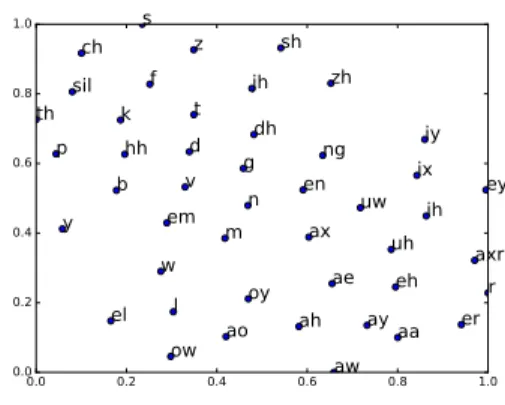
0.0 0.2 0.4 0.6 0.8 1.0 0.0 0.2 0.4 0.6 0.8 1.0 en ax axr v aa r ay th ae ah eh m sh g ey zh s w ch k jh _iy el em l sil uw p ng aooy uh ow _aw f dh dt bhh ih er ix z y n

Fig. 2. WSJ-SI84 2-dimensional Mapping of English Phonemes via t-SNE. For systems with activation regularisation, each layer formed a32×32grid. For the KL and Cos systems, 46 English phones were used to define the time-variant target patterns, and 2D positions of the phones were estimated via the t-SNE method over the average of frames of different phones. They were then scaled to fit in a unit square[0,1]×[0,1]. Figure 2 illustrates the 2D projection of the phones. The regularisation parameters were empirically tuned on the development data H1-Dev. For the Cos and Smooth systems, sigmoid, ReLU and hyperbolic tangent activation functions were investigated. For the KL system, only sigmoid activation function was used. 1_{Dropout regularisation does not yield gains in the configuration evaluation}

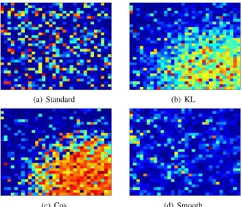
Figure 3 shows the outputs of the third-hidden-layer activa-tion grid of standard (no addiactiva-tional regularisaactiva-tion), KL, Cos and Smooth sigmoid DNNs for an ”aa” frame sample.2_{. As} expected, both the KL and Cos DNNs yielded the target pat-terns: the activation functions around the phone “aa” location

(a) Standard (b) KL

(c) Cos (d) Smooth

Fig. 3. Comparison of Standard (No Additional Regularisation), KL, Cos and Smooth DNN Activation Function Outputs on an “aa” Frame.

echoed higher values than other regions. The Smooth DNN, which does not have a specific target, just yielded a smoothed pattern.

The impact of the normalised activation, as defined in Eq. 15, is shown in Table I. By using this transform instead

TABLE I

WSJ-SI84 IMPACT OFNORMALISEDACTIVATION(NORMACT)ON SIGMOIDDNNS ONH1-DEV

R _{NormAct WER (%)}

L2 – 10.0

KL ₃7 9.9

9.7

of raw activation function outputs in the regularisation term, the KL system could further reduce the word error rate (WER). Similar results were also found in the Cos and Smooth DNNs. Table II compares the impact of different η and σ

TABLE II

WSJ-SI84 COMPARISON OFηANDσ2OFKL-REGULARISED SIGMOID DNNS ONH1-DEV[WER (%)] P P P P PP σ2 η 0.1 0.2 0.3 0.5 0.05 10.0 9.9 – – 0.1 9.9 9.7 10.1 10.6 0.2 9.9 9.8 – –

configurations in the KL regularisation. The best performance was achieved by settingη to 0.2 andσ2_{to 0.1. Withσ}2_{= 0.1}

2_{An example video, showing the activation function outputs of one}

sen-tence, is provided at http://mi.eng.cam.ac.uk/˜cw564/stimulated/example.avi.

and a32×32grid, approximately 322 activation functions are within one standard deviation of the stimulation point for a particular phone. This is the region most heavily influenced

0.0 0.1 0.2 0.3 0.4 Regularisation Penalty 1.30 1.35 1.40 1.45 1.50 1.55 Cross Entropy CE 0 5 10 15 20 25 KL-divergence KL

Fig. 4. WSJ-SI84 Cross-entropy and KL-divergence Values of the CV Set on Different Regularisation Penalties.

by this form of regularisation term. Figure 4 illustrates the cross entropy and KL-divergence values of the cross validation set, which can be viewed as an indicator of the generalised performance, for different η settings and a fixed value ofσ2

at 0.1. Higher values of η resulted in lower KL-divergence values. The cross-entropy initially decreased (improved), but then increased in value with higher values ofη. The minimal cross-entropy value was achieved when η was in the range between 0.1 and 0.3, which is consistent with the optimal decoding performance on H1-Dev.

Tables III and IV summarises the decoding performance of different DNNs on theH1-DevandH1-Evaltestsets. The

TABLE III

WSJ-SI84 SYSTEMSUMMARY ONH1-DEV[WER (%)]

R _{Sigmoid ReLU Tanh}

L2 10.0 10.9 10.5 Dropout 10.0 – – KL 9.7 – – Cos 9.7 10.5 10.5 Smooth 9.8 10.8 10.4 TABLE IV

WSJ-SI84 SYSTEMSUMMARY ONH1-EVAL[WER (%)]

R Sigmoid ReLU Tanh

L2 10.2 10.9 11.2

Dropout 10.0 – –

KL 10.0 – –

Cos 10.1 10.8 11.0

Smooth 10.1 10.8 10.9

Cos and Smooth regularisation on sigmoid, ReLU and tanh DNNs yielded similar performance. On this relatively small task, small consistent gains could be obtained. On the H1-Eval, the proposed methods slightly outperformed the dropout regularisation; however, they yielded similar results as the dropout on H1-Dev.

B. Babel Languages

Experiments in this section were conducted on seven devel-opment languages and one surprise language from the IARPA

Babel program in the option period3 _{3. For all the languages,} an automatic, unicode-based, graphemic dictionary generation [33] was applied. The “pure” graphemes were extended with position information and language dependent attributes. The full language pack (FLP) dataset was used for each language. It consisted of 40 hours of conversational telephone speech (CTS). An additional 10-hour development dataset was used as the testset.

Two language models were used in these experiments: the n-gram LM and the recurrent neural networks (RNN) LM trained using the CUED RNN LM toolkit [34]. These were both trained on acoustic data transcripts containing approx-imately 500k words. Additional n-gram LMs were trained on data collected from the web [35]. These web LMs were then interpolated with the FLP LMs by optimising inter-polation weights on the development data. Acoustic models were speaker adaptively trained Tandems [36] and (stacked) Hybrids [37] that shared the same set of features. The DNN input features were formed as concatenating PLP, pitch [38], probability of voicing [38] and multi-language bottleneck fea-tures [39] provided by IBM and RWTH Aachen, in a temporal context window of 9 frames. Thus, a total of 4 acoustic models was built for each language. Stacked Hybrids were trained us-ing mono-phone discriminative pre-trainus-ing initialisation and followed by cross-entropy training and minimum-phone-error training, with and without the activation regularisation. Unless otherwise stated, KL regularisation was used; 5 hidden layers with a 32×32 grid in each layer were used. The grid for activation regularisation was built using the sets of graphemes extended with position information and attributes. To achieve high transcription accuracy, the final system combined the 4 acoustic models, two hybrid and two tandem, via a joint decoding [40]. Note no activation regularisation was used for the tandem systems. More details of this joint system can be found in [41]. Keyword search was performed using the joint decoding lattices. About 2k keywords were available for each language [42]. The performance was measured by the maximum term weighted value (MTWV) [43].

The first experiment compared these regularisation config-urations on Javanese with a simplified configuration. A single DNN using the RWTH multi-language bottleneck features was investigated, and decoding was performed using a tri-gram LM. Again sigmoid, ReLU and tanh activation functions

TABLE V

CE DECODINGSUMMARY ONJAVANESE[WER (%)]

R _{Sigmoid ReLU Tanh}

L2 58.2 59.2 58.5

KL 57.2 – –

Cos 57.9 59.0 57.9

Smooth 57.9 58.9 58.0

were investigated in different regularisation schemes. The recognition performance of the CE systems is compared in 3_{Pashto babel104b-v0.4bY, Guarani babel305b-v1.0a, Igbo}

IARPA-babel306b-v2.0c, Amharic IARPA-babel307b-v1.0b, Mongolian IARPA-babel401b-v2.0b, Javanese IARPA-babel402b-v1.0b, Dholuo IARPA-babel403b-v1.0b, Georgian IARPA-babel404b-v1.0a

Table V. On different activation function settings, Cos and Smooth DNNs outperformed their corresponding baselines. The sigmoid function yielded better performance than other activation functions, and the best system was the KL sigmoid DNN. These sigmoid CE systems were further tuned using the MPE criterion. Table VI shows the performance of dif-ferent MPE DNNs. The MPE training on difdif-ferent systems

TABLE VI

DECODINGSUMMARY OFCEANDMPE SIGMOIDDNNS ONJAVANESE [WER (%)] R _{CE MPE} L2 58.2 56.5 KL 57.2 55.8 Cos 57.9 56.2 Smooth 57.9 56.3

yielded lower-error performance than their corresponding CE baselines. Similar to CE systems, the best performance was achieved by the KL system, reducing the token error rate from 56.5% to 55.8%.

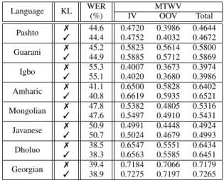
The second experiment contrasted standard and KL systems on all languages in more advanced configuration combining 4 acoustic models and interpolated FLP and web data LMs in a single joint decoding run. The overall MTWV results are presented alongside in-vocabulary (IV) and out-of-vocabulary (OOV) query only results. The results in Table VII show that

TABLE VII

COMPARISON OFSTANDARDDNNANDKL REGULARISEDSYSTEMS ON ALLLANGUAGES

Language KL WER_{(%) IV} MTWV_{OOV Total} Pashto ₃7 44.6 0.4720 0.3986 0.4644 44.4 0.4752 0.4032 0.4672 Guarani ₃7 45.2_44.9 0.5823_0.5885 0.5614_0.5712 0.5800_0.5869 Igbo ₃7 55.3 0.4007 0.3673 0.3974 55.1 0.4020 0.3680 0.3986 Amharic ₃7 41.1_40.8 0.6500_0.6619 0.5828_0.5935 0.6402_0.6521 Mongolian ₃7 47.8 0.5382 0.4805 0.5316 47.6 0.5497 0.4910 0.5431 Javanese ₃7 50.9_50.7 0.4991_0.5024 0.4448_0.4679 0.4924_0.4993 Dholuo ₃7 38.5 0.6547 0.5551 0.6434 38.3 0.6563 0.5585 0.6451 Georgian ₃7 39.4_38.9 0.7184_0.7275 0.7066_0.7197 0.7179_0.7265

ASR gains are seen even after system combination for all languages. Similarly, gains can be seen in KWS performance for all languages.

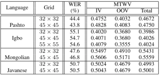
The third experiment assessed whether activation regular-isation scaled with increasing the grid size on the 4 most challenging languages. Experiments have so far examined a 32×32 grid. A larger 45×45 grid was examined for all languages plus an even larger 55 ×55 grid for the most challenging language. The use of a larger 45×45 grid in Table VIII shows ASR and KWS gains for all languages. Further increase in the grid size, 55 ×55, for the most challenging language Igbo, yielded little benefit. The results

TABLE VIII

IMPACT OFGRIDSIZE OFKL SYSTEMS ONFOURMOSTCHALLENGING LANGUAGES

Language Grid WER MTWV

(%) IV OOV Total Pashto 32×32 _{44.4 0.4752 0.4032 0.4672} 45×45 _{43.8 0.4828 0.4083 0.4750} Igbo 32×32 _{55.1 0.4020 0.3680 0.3986} 45×45 _{54.7 0.4071 0.3680 0.4026} 55×55 _{54.6 0.4079 0.3555 0.4024} Mongolian 32×32 _{47.6 0.5497 0.4910 0.5431} 45×45 _{46.8 0.5606 0.5171 0.5559} Javanese 32×32 _{50.7 0.5024 0.4679 0.4993} 45×45 _{50.5 0.5043 0.4679 0.5001}

in Tables VII and VIII show the advantages of activation regularisation, which results in ASR and KWS gains in all examined languages.

C. Broadcast News

This task used the 144-hour 1996 and 1997 Hub-4 English Broadcast News Speech dataset (LDC97S44, LDC98S71), containing 288 shows from approximately 8k speakers. Two testsets were used for the evaluation: the 2.7-hour Dev03 and 2.6-hour Eval03. The utterances of both testsets were processed by automatic segmentation, and their averaged ut-terance durations were 10.7 and 10.9 seconds, respectively. Decoding was performed with a tri-gram language model. Related settings are described in more detail in [44].

For DNN models, the sigmoid activation function was examined. The baseline DNN cross-entropy system used the 468-dimensional PLP+∆+∆∆+∆∆∆ features, processed by both global CMN and CVN, in a temporal context window of 9 frames as the input feature. The network consisted of 5 hidden layers, and each layer formed a default32×32grid. The DNN parameters were initialised in the layer-wise discriminative pre-training fashion and then optimised by back-propagation on the CE criterion. This CE DNN baseline was further trained on the MPE criterion.

For activation regularisation, the default English phone set was used, and phone positions were obtained via t-SNE over the training-set averaged frames of the phones. Regularisation parameters were again empirically tuned on the development data Dev03.

Table IX summarises the performance of different CE systems. Three systems using activation regularisation out-performed their respective DNN baselines. The KL system showed the best performance, which reduced the relative WER up to 5% in contrast with the CE DNN baseline. The CE KL

TABLE IX

CE SIGMOIDDNN PERFORMANCE ONBROADCASTNEWS[WER (%)]

R _{Dev03 Eval03} L2 12.5 10.7 KL 11.9 10.3 Cos 12.3 10.6 Smooth 12.2 10.7 TABLE X

MPE SIGMOIDDNN PERFORMANCE ONBROADCASTNEWS[WER (%)]

R _{Dev03 Eval03}

L2 11.6 10.1

KL 11.2 9.8

system was then further tuned on the MPE criterion. Similar to the CE ones, the MPE KL system outperformed the MPE baseline as illustrated in Table X, reducing the WER up to 4% relatively.

V. CONCLUSION

This paper presents a general framework for activation regularisation to improve interpretability and regularisation in deep learning models. This framework allows appropriate target patterns to be interpreted on activation function outputs. The target patterns are introduced to induce desired infor-mation such as different learning concepts or smoothness. A regularisation term is added to the cost function, which encourages activation outputs to perform similarly to the target pattern. In this way, network interpretation can be easily deduced from the visualisation of activation function outputs. Furthermore, they give the potential to reduce over-fitting and aid DNN generalisation. The proposed methods were evaluated on three tasks: the Wall Street Journal continuous speech recognition task, eight conversational telephone speech tasks from the IARPA Babel program and a U.S. English broadcast news task. The activation regularisation has shown consistent performance gains in contrast with their corresponding DNN baselines. Future work will look at activation regularisation on more complex network topologies such as recurrent neural networks and further adaptation methods that utilises informa-tion in activainforma-tion output patterns.

REFERENCES

[1] C. Wu, P. Karanasou, M. J. Gales, and K. C. Sim, “Stimulated deep neural network for speech recognition,” inProc. Interspeech, 2016, pp. 400–404.

[2] A. Ragni, C. Wu, M. Gales, J. Vasilakes, and K. Knill, “Stimulated training for automatic speech recognition and keyword search in lim-ited resource conditions,” in Acoustics, Speech and Signal Processing (ICASSP), 2017 IEEE International Conference on. IEEE, 2017, pp. 4830–4834.

[3] G. E. Dahl, D. Yu, L. Deng, and A. Acero, “Context-dependent pre-trained deep neural networks for large-vocabulary speech recognition,”

Audio, Speech, and Language Processing, IEEE Transactions on, vol. 20, no. 1, pp. 30–42, 2012.

[4] G. Hinton et al., “Deep neural networks for acoustic modeling in speech recognition: The shared views of four research groups,”Signal Processing Magazine, IEEE, vol. 29, no. 6, pp. 82–97, 2012. [5] W. Xiong, J. Droppo, X. Huang, F. Seide, M. Seltzer, A. Stolcke,

D. Yu, and G. Zweig, “Achieving human parity in conversational speech recognition,” CoRR, vol. abs/1610.05256, 2016. [Online]. Available: http://arxiv.org/abs/1610.05256

[6] N. Srivastava, G. E. Hinton, A. Krizhevsky, I. Sutskever, and R. Salakhutdinov, “Dropout: a simple way to prevent neural networks from overfitting.”Journal of Machine Learning Research, vol. 15, no. 1, pp. 1929–1958, 2014.

[7] S. Ioffe and C. Szegedy, “Batch normalization: Accelerating deep network training by reducing internal covariate shift,” inInternational Conference on Machine Learning, 2015, pp. 448–456.

[8] Y. LeCun, L. Bottou, Y. Bengio, and P. Haffner, “Gradient-based learning applied to document recognition,” Proceedings of the IEEE, vol. 86, no. 11, pp. 2278–2324, 1998.

[9] A. Krizhevsky, I. Sutskever, and G. E. Hinton, “Imagenet classification with deep convolutional neural networks,” inAdvances in neural infor-mation processing systems, 2012, pp. 1097–1105.

[10] R. Collobert and J. Weston, “A unified architecture for natural language processing: Deep neural networks with multitask learning,” in Proceed-ings of the 25th international conference on Machine learning. ACM, 2008, pp. 160–167.

[11] M. L. Seltzer and J. Droppo, “Multi-task learning in deep neural net-works for improved phoneme recognition,” in2013 IEEE International Conference on Acoustics, Speech and Signal Processing. IEEE, 2013, pp. 6965–6969.

[12] P. Bell and S. Renals, “Regularization of context-dependent deep neural networks with context-independent multi-task training,” in2015 IEEE International Conference on Acoustics, Speech and Signal Processing (ICASSP). IEEE, 2015, pp. 4290–4294.

[13] C. M. Bishop, “Mixture density networks,” 1994.

[14] E. Variani, E. McDermott, and G. Heigold, “A gaussian mixture model layer jointly optimized with discriminative features within a deep neural network architecture,” in 2015 IEEE International Conference on Acoustics, Speech and Signal Processing (ICASSP). IEEE, 2015, pp. 4270–4274.

[15] S. Zhang, H. Jiang, and L. Dai, “Hybrid orthogonal projection and estimation (HOPE): A new framework to learn neural networks,”Journal of Machine Learning Research, vol. 17, no. 37, pp. 1–33, 2016. [16] C. Wu and M. J. Gales, “Multi-basis adaptive neural network for rapid

adaptation in speech recognition,” in Acoustics, Speech and Signal Processing (ICASSP), 2015 IEEE International Conference on. IEEE, 2015, pp. 4315–4319.

[17] C. Wu, P. Karanasou, and M. J. Gales, “Combining i-vector representa-tion and structured neural networks for rapid adaptarepresenta-tion,” inAcoustics, Speech and Signal Processing (ICASSP), 2016 IEEE International Conference on. IEEE, 2016, pp. 5000–5004.

[18] A. Goh, “Back-propagation neural networks for modeling complex systems,”Artificial Intelligence in Engineering, vol. 9, no. 3, pp. 143– 151, 1995.

[19] A. Nguyen, J. Yosinski, and J. Clune, “Deep neural networks are easily fooled: High confidence predictions for unrecognizable images,” inProceedings of the IEEE Conference on Computer Vision and Pattern Recognition, 2015, pp. 427–436.

[20] A. Mahendran and A. Vedaldi, “Understanding deep image represen-tations by inverting them,” inProceedings of the IEEE Conference on Computer Vision and Pattern Recognition, 2015, pp. 5188–5196. [21] K. Simonyan, A. Vedaldi, and A. Zisserman, “Deep inside convolutional

networks: Visualising image classification models and saliency maps,”

arXiv preprint arXiv:1312.6034, 2013.

[22] M. D. Zeiler and R. Fergus, “Visualizing and understanding convolu-tional networks,” inEuropean conference on computer vision. Springer, 2014, pp. 818–833.

[23] K. Kavukcuoglu, R. Fergus, Y. LeCunet al., “Learning invariant features through topographic filter maps,” in Computer Vision and Pattern Recognition, 2009. CVPR 2009. IEEE Conference on. IEEE, 2009, pp. 1605–1612.

[24] D. Povey and P. C. Woodland, “Minimum phone error and i-smoothing for improved discriminative training,” inAcoustics, Speech, and Signal Processing (ICASSP), 2002 IEEE International Conference on, vol. 1. IEEE, 2002, pp. I–105.

[25] P. Swietojanski and S. Renals, “Learning hidden unit contributions for unsupervised speaker adaptation of neural network acoustic models,” inSpoken Language Technology Workshop (SLT), 2014 IEEE. IEEE, 2014, pp. 171–176.

[26] S. Tan, K. C. Sim, and M. Gales, “Improving the interpretability of deep neural networks with stimulated learning,” inAutomatic Speech Recognition and Understanding (ASRU), 2015 IEEE Workshop on. IEEE, 2015, pp. 617–623.

[27] L. Van der Maaten and G. Hinton, “Visualizing data using t-SNE,”

Journal of Machine Learning Research, vol. 9, no. 2579-2605, p. 85, 2008.

[28] J. Garofalo, D. Graff, D. Paul, and D. Pallett, “CSR-I (WSJ0) complete,”

Linguistic Data Consortium, Philadelphia, 2007.

[29] M. Harper, “The babel program and low resource speech technology,”

Proc. of ASRU 2013, 2013.

[30] D. Graff, “The 1996 broadcast news speech and language-model corpus,” inProc. 1997 DARPA Speech Recognition Workshop, 1997, pp. 11–14.

[31] D. S. Pallett, J. G. Fiscus, A. Martin, and M. A. Przybocki, “1997 broadcast news benchmark test results: English and non-English,” in

Proc. 1998 DARPA Broadcast News Transcription and Understanding Workshop, 1998, pp. 5–11.

[32] S. Young, G. Evermann, M. Gales, T. Hain, D. Kershaw, X. A. Liu, G. Moore, J. Odell, D. Ollason, D. Povey, A. Ragni, V. Valtchev, P. Woodland, and C. Zhang, “The HTK book (for HTK version 3.5),” 2015.

[33] M. J. F. Gales, K. M. Knill, and A. Ragni, “Unicode-based graphemic systems for limited resource languages,” inICASSP, 2015.

[34] X. Chen, X. Liu, Y. Qian, M. J. F. Gales, and P. C. Woodland, “CUED-RNNLM – an open-source toolkit for efficient training and evaluation of recurrent neural network language models,” inICASSP, 2016. [35] G. Mendels, E. Cooper, V. Soto, J. Hirschberg, M. Gales, K. Knill,

A. Ragni, and H. Wang, “Improving speech recognition and keyword search for low resource languages using web data,” inInterspeech, 2015. [36] H. Hermansky, D. P. Ellis, and S. Sharma, “Tandem connectionist feature extraction for conventional HMM systems,” inAcoustics, Speech, and Signal Processing, 2000. ICASSP’00. Proceedings. 2000 IEEE International Conference on, vol. 3. IEEE, 2000, pp. 1635–1638. [37] A.-r. Mohamed, G. E. Dahl, and G. Hinton, “Acoustic modeling

us-ing deep belief networks,” IEEE Transactions on Audio, Speech, and Language Processing, vol. 20, no. 1, pp. 14–22, 2012.

[38] P. Ghahremani, B. BabaAli, D. Povey, K. Riedhammer, J. Trmal, and S. Khudanpur, “A pitch extraction algorithm tuned for automatic speech recognition,” inICASSP, 2014.

[39] Z. Tuske, D. Nolden, R. Schluter, and H. Ney, “Multilingual mrasta features for low-resource keyword search and speech recognition sys-tems,” inAcoustics, Speech and Signal Processing (ICASSP), 2014 IEEE International Conference on. IEEE, 2014, pp. 7854–7858.

[40] H. Wang, A. Ragni, M. J. F. Gales, K. M. Knill, P. C. Woodland, and C. Zhang, “Joint decoding of tandem and hybrid systems for improved keyword spotting on low resource languages,” inInterspeech, 2015. [41] A. Ragni, C. Wu, M. Gales, J. Vasilakes, and K. Knill, “Stimulated

training for automatic speech recognition and keyword search in limited resource conditions.”

[42] J. Cui, J. Mamou, B. Kingsbury, and B. Ramabhadran, “Automatic keyword selection for keyword search development and tuning,” in

ICASSP, 2014.

[43] J. G. Fiscuset al., “Results of the 2006 spoken term detection eval-uation,” in Proc. ACM SIGIR Workshop on Searching Spontaneous Conversational Speech, 2007.

[44] S. Tranter, M. Gales, R. Sinha, S. Umesh, and P. Woodland, “The development of the Cambridge University RT-04 diarisation system,” inProc. Fall 2004 Rich Transcription Workshop (RT-04), 2004.