Coupled CFD
–
DEM simulation of
fl
uid
–
particle interaction in geomechanics
Jidong Zhao
⁎
, Tong Shan
Department of Civil and Environmental Engineering, The Hong Kong University of Science and Technology, Clear Water Bay, Kowloon, Hong Kong
a b s t r a c t
a r t i c l e i n f o
Article history: Received 12 June 2012
Received in revised form 7 November 2012 Accepted 2 February 2013
Available online 8 February 2013 Keywords:
Granular media Fluid–particle interaction Coupled CFD–DEM Single particle settling 1D consolidation Sandpile
This paper presents a coupled Computational Fluid Dynamics and Discrete Element Method (CFD–DEM) approach to simulate the behaviour offluid–particle interaction for applications relevant to mining and geotechnical engineering. DEM is employed to model the granular particle system, whilst the CFD is used to simulate thefluidflow by solving the locally averaged Navier–Stokes equation. The particle–fluid interac-tion is considered by exchanging such interacinterac-tion forces as drag force and buoyancy force between the DEM and the CFD computations. The coupled CFD–DEM tool isfirst benchmarked by two classic geomechanics problems where analytical solutions are available, and is then employed to investigate the characteristics of sand heap formed in water through hopperflow. The influence offluid–particle interaction on the behav-iour of granular media is well captured in all the simulated problems. It is shown in particular that a sand pile formed in water is more homogeneous in terms of void ratio, contact force and fabric anisotropy. The central pressure dip of vertical stress profile at the base of sandpile is moderately reduced, as compared to the dry case. The effects of rolling resistance and polydispersity in conjunction with the presence of water on the formation of sandpile are also discussed.
© 2013 Elsevier B.V. All rights reserved.
1. Introduction
Fluid–particle interaction underpins the performance of a wide range of key engineering applications relevant to granular media. Subjected to external loads, the porefluid in a saturated granular ma-terial mayfluctuate orflow and cause particle motion. This may work favourably in some cases, such as in sand production in sandstone oil reservoir, but may be an adverse factor in other occasions, such as in the case of internal/surface erosion of embankment dams and soil slopes which may trigger instability and failure of these struc-tures[21]. Conventional approaches based on continuum theories of porous media, such as the Biot theory, have considered the interac-tion between porefluids and particles in a phenomenological man-ner. They cannot offer microscopic information at the particle level relevant to the fluid–particle interaction which may be otherwise useful in many occasions. Indeed, as mentioned in a recent review by Zhu et al.[38], a quantitative understanding of the microscale phenomena relative tofluid–particle interaction could facilitate the establishment of general methods for reliable scale-up, design and control of different particulate systems and processes. To this end, a number of collective attempts have been made on particle-scale modelling offluid–particle interaction, among which Discrete Element
Method (DEM) plays a central role. In particular, numerical approaches combining the Computational Fluid Dynamics and Discrete Element Method (CFD–DEM) prove to be advantageous over many other op-tions, such as the Lattice–Boltzman and DEM coupling (LB–DEM) meth-od and the Direct Numerical Simulation coupled DEM (DNS–DEM), in terms of computational efficiency and numerical convenience [37]. A typical CFD–DEM method solves the Newton's equations governing the motion of the particle system by DEM and the Darcy's law or the Navier–Stokes equation for thefluidflow by CFD, in consideration of proper interaction force exchanges between the DEM and the CFD (see[21,27,32,33,37]). The method has been successfully applied to the simulation of applications such asfluidization, pneumatic convey-ing and pipelineflow, blast furnace, cyclone, andfilm coating (see the review by[38]).
Relevant to civil and geotechnical engineering, the important impact offluid–particle interaction on the overall behaviour of soils has long been recognized. More recently, there has been a growing interest in exploring the soil behaviour using discrete modelling approaches, in sought for key mechanisms and mitigating measures for various geotechnical hazards (see[21]for a summary). Whilst the majority of these studies were focused on the dry soil case based on DEM only, there have been limited investigations considering thefluid–particle interaction through coupled discrete approaches as mentioned before. A handful of exceptions include the treatment of upward seepageflow in soils, sinkhole process,flow under sheet pile walls [6,7,25]. The current paper aims to develop a coupled CFD– DEM numerical tool to investigate various geomechanics problems ⁎ Corresponding author. Fax: +852 2358 1534.
E-mail address:[email protected](J. Zhao).
0032-5910/$–see front matter © 2013 Elsevier B.V. All rights reserved.
http://dx.doi.org/10.1016/j.powtec.2013.02.003
Contents lists available atSciVerse ScienceDirect
Powder Technology
relevant to mining and geotechnical engineering. In particular, two open-source DEM and CFD packages are employed to facilitate the coupling betweenfluids and particles, namely, the LAMMPS-based
DEM code, LIGGGHTS [16], and the OpenFOAM (www.openfoam.
com). The computational framework has been based on the CFDEM program developed by Goniva et al.[13], by further considering both phases of gas and water in thefluid simulation by OpenFOAM. The
fluid–particle coupling is considered by exchanging interaction forces between the two packages during the computation. The interaction forces being considered include the drag force and buoyancy force, which may generally suffice for granular materials in geomechanics with relatively low Reynolds number of poreflow. Such complex interaction forces as unsteady forces like virtual mass force, Basset force and lift forces and non-contact forces such as capillary force, Van der Waals force and electrostatic force, may be important for certain applications, but will not be considered here. It is however emphasized that the computational framework is general and can easily accommodate the consideration of these forces if necessary in the future.
Three problems will be employed to demonstrate the predictive capacity of the numerical tool. They include the single-particle settling in water which simulates a typical sedimentation process, the one-dimensional consolidation and the formation of conical sand pile through a hopper into water. Thefirst two examples are chosen due not only to their simplicity but also the availability of analytical solutions for both, and consequently, they serve as benchmarks for the developed CFD– DEM package. The sand pile formation problem has received much atten-tion in a wide range of branches of engineering and science. Of particular interest is the phenomenon of pressure dip in sandpile observed in experiments. Various analytical approaches and numerical studies have been devoted to the explanation of this phenomenon, such as thefixed principal axes model[31], the arching theory based on limit analysis by Michalowski and Park[20], as well as DEM simulations[12,17]. The occurrence of pressure dip in sandpile has been found dependent on the construction method, particle shape and other factors[1,39]. Despite the intensive studies on this topic, no widely accepted consensus has been reached regarding the major mechanism for the observed pres-sure dip. In particular, very scarce studies have been found exploring the effect of water on the formation of a sandpile and on the charac-teristics of the pressure dip. Relevant studies in this respect may have a far wider engineering background closely related to such is-sues as dredging and land reclamation, mining production handling, soil erosion and debrisflow wherein the interaction between soil and water proves to be important. The CFD–DEM tool developed in this paper will be employed to investigate the characteristics of sandpile formed through hopperflow in water, and careful compar-ison will be made against the dry case.
2. Methodology and formulation
Key to the coupling between the Computational Fluid Dynamics method and Discrete Element Method (CFD–DEM) is proper consid-eration of particle–fluid interaction forces. Typical particle–fluid in-teraction forces considered in past studies include the buoyancy force, pressure gradient force, drag force due to the particle motion resistance by stagnantfluid, as well as other unsteady forces such as virtual mass force, Basset force and lift forces (see,[37]). Following the approach proposed by Tsuji et al.[27,28], we assume that the motion of particles in the DEM is governed by the Newton's laws of motion and the porefluid is continuous which can be described by locally averaged Navier–Stokes equation to be solved by the CFD[3]. The interactions between thefluid and the particles are modelled by exchange of drag force and buoyancy force only. Detailed formalisms governing the three aspects and numerical solution procedures are described as follows.
2.1. Governing equations for the porefluid and particle system
For a particleitreated by the DEM[9], the following equations are assumed to govern its translational and rotational motions
mi dUpi dt ¼ Xnc i j¼1 FcijþF f iþF g i Ii dωi dt ¼ Xnc i j¼1 Mij 8 > > > > > < > > > > > : ð1Þ
whereUipandωidenote the translational and angular velocities of particlei, respectively.FijcandMijare the contact force and torque act-ing on particleiby particlejor the wall(s), andnicis the number of total contacts for particlei.Fifis the particle–fluid interaction force acting on particlei, which includes both buoyancy force and drag force in the current case.Figis the gravitational force.miandIiare the mass and moment of inertia of particlei. In the DEM code, either the Hooke or Hertzian contact law is employed in conjunction with Coulomb's friction law to describe the interparticle contact behaviour.
In the CFD method, the continuousfluid domain is discretized into cells. In each cell variables such asfluid velocity, pressure and density are locally averaged quantities. In particular, a specific cell can be occu-pied by immiscible liquid and air, and the density of a cell is the weight-ed average of the two phases (excluding the volume of particles if they are present in a cell). The following continuity equation is assumed to hold for each cell:
∂ð Þερ
∂t þ∇⋅ ερU
f
¼0 ð2Þ
whereUfis the average velocity of afluid cell.ε=vvoid/vc= 1−vp/vc denoting the porosity (void fraction) (vvoidis the total volume of void in a cell which may contain either air or water or both;vpis the volume occupied the particle(s) in a cell;vcis the total volume of a cell).ρis the averagedfluid density defined by:ρ=αρw+ (1−α)ρa, whereα=vw/ vc= 1−va/vc.αis defined in the CFD simulation by thenominal vol-ume fraction of water phase in a cell, where vw is the nominal water phase volume in the cell andvathe nominal air phase volume, andvw+va=vc. Evidently, the total void volume in a cell can be written asvvoid=ε(va+vw). Ifα= 1, the void of a cell will be fully oc-cupied by water, and ifα= 0, the void is full of air. The case of 0bαb1 normally refers to a cell with voidfilled by both air and water. This def-inition of averagefluid density in conjunction with the porosityεleads to a neatly expressed continuity equation in Eq.(2), and has been wide-ly followed. In addition, as will be shown, this definition offers a conve-nient way to simulate the transition process of particles passing between the interface between (pure) air phase and water phase. The CFD method solves the following locally averaged Navier–Stokes equa-tion in conjuncequa-tion with the continuity equaequa-tion in Eq.(2)
∂ερUf ∂t þ∇⋅ ερU f Uf −ε∇⋅μ∇Uf¼−∇p−fpþερg ð3Þ wherepis thefluid pressure in the cell;μis the averaged viscosity;fp is the interaction force averaged by the cell volume the particles inside the cell exert on thefluid.gis the gravitational acceleration.
2.2. Fluid–particle interaction forces
The motion of submerged particles can be significantly influenced by thefluid through either hydrostatic or hydrodynamic forces. Buoy-ancy force is a typical hydrostatic force, whilst hydrodynamic forces may include drag force, the virtual mass force and the lift force,
among others[21,37]. In this study, we consider the drag forceFdand the buoyancy forceFbas the dominant interaction forces. Specifically, the expression of drag force used by Di Felice[11]is employed:
Fd¼18Cdρπd 2 p U f −Up Uf−Up ε1−χ ð4Þ
wheredpis the diameter of the considered particle.Cdis the particle–
fluid drag coefficient which depends on the Reynolds number of the particle, Rep Cd¼ 0:63þ 4:8 ffiffiffiffiffiffiffiffi Rep q 0 B @ 1 C A 2 ð5Þ
in which the particle Reynolds number is determined by:
Rep¼ ερdpU f −Up μ : ð6Þ
ε−χin Eq.(4)denotes a corrective function to account for the presence
of other particles in the system on the drag force of the particle under consideration, whereinχhas the following expression
χ¼3:7−0:65 exp − 1:5−log10Rep 2 2 2 6 4 3 7 5: ð7Þ
As indicated by Kafui et al.[15], the Di Felice expression leads to a smooth variation in the drag force as a function of porosity. The expressions in Eqs.(4) and (5)work well for our applications with relatively low Reynolds numbers.
Regarding the hydrostatic force, we employ the following average density based expression for the buoyancy force (c.f.[15,21]):
Fb¼16πρd3pg: ð8Þ
2.3. Numerical solution schemes for coupled CFD–DEM computation
In the coupled CFD–DEM scheme, thefluid phase is discretized with a typical cell size several times of the average particle diameter. At each time step, the DEM package provides such information as the position and velocity of each individual particle. The positions of all particles are then matched with thefluid cells to calculate relevant information of each cell such as the porosity. By following the coarse-grid approximation method proposed by Tsuji et al.[27], the locally-averaged Navier–Stokes equation in Eq.(3)is solved by the CFD program for the averaged velocity and pressure for each cell. The obtained averaged values for the velocity and pressure of a cell are then used to determine the drag force and buoyancy force acting on the particles in that cell. Iterative schemes may have to be invoked to ensure the convergence of relevant quantities such as thefluid velocity and pressure. When a converged solution is obtained, the information offluid–particle interaction forces will be passed to the DEM for the next step calculation. LIGGGHTS has been adopted as the DEM package and thefinite-volume-method based OpenFOAM code is employed as the CFD solver. A customized OpenFOAM library, CFDEM, developed by Goniva et al.[13], has been modified to wrap the OpenFOAMfluid solver into the LIGGGHTS solution procedure to solve the coupled problem. The InterDyMFoam solver is modified in the OpenFOAM to solve the locally averaged Navier–Stokes equation.
Ideally, information on interaction forces should be exchanged imme-diately after each step of calculation for the DEM or the CFD. This, however, may request excessive computational effort in practice. For the problems to be treated in this paper, numerical experience shows that for each CFD computing step, exchanging information after 100 steps of DEM calculation will ensure sufficient accuracy and efficiency. If the time steps for DEM and CFD are sufficiently small, more steps for DEM are also acceptable.
2.4. Two approaches calculating the void fraction of afluid cell
The CFD–DEM method employed here generally considers afluid cell with a size several times of the mean particle diameter. It is inter-esting to compare two different methods in calculating the void frac-tion for afluid cell which are shown in Fig. 1in a demonstrative 2D view (our code is 3D).Fig. 1a illustrates thecentre void fraction
method. In this method, if the centre of a particleiis found located
in afluid cellj, the total volume of the particle will be counted into the calculation of the void fraction for that cell. For example, Particles A,B,CandDinFig. 1a will all be counted into the calculation of void fraction for Cell 2. Whilst for the case of Particle E, it can be considered either entirely to Cell 2 or Cell 4, but not both. Apparently, this approach will overestimate the void fraction for some cells whilst underestimating it for others in the neighbourhood. An improved method is shown inFig. 1b, where the exact volume fraction of a par-ticleiin afluid cellj,ϖij, is accurately determined (ϖij=vijp/vip, where vip is the total volume of particle i and vijp is the exact portion of volume of particleiin cellj). Evidently,ϖij∈[0,1]. When a particle is entirely located in Cellj (such as the case of Particles B and C with respect to Cell 2),ϖij= 1; when it is totally outside that cell, ϖij= 0. Otherwise, its value is in between 0 and 1.ϖijis then used to calculate the void fraction of the concerned cells. The latter ap-proach is termed as thedivided void fraction method. Evidently, the
first approach can be regarded as a special case of the second, with ϖij either equal to 1 or 0, depending on its centroid location with respect to the cell.
The two approaches affect how the fluid–particle interaction forces are calculated. In calculating the interaction force applied to a DEM particlei, a simplified centre-position approach (similar to the centre void fraction method mentioned above) has been followed for all cases. Specifically, the averagefluid velocityUfin Eq.(4)and the averagefluid densityρin both Eqs.(4) and (8)are chosen entirely according to the cell the particle centre is located in. As such, the total interaction force applied to particleiis
Ffi ¼F d i þF b i: ð9Þ
a
b
Fig. 1.Schematic of two different approaches to calculate the void fraction for afluid cell. (a) The centre void fraction method; (b) the divided void fraction method.
This expression is followed in both the centre and the divided void fraction methods. However, in calculating the interaction forces for a
fluid cellj, the contributing weight of each particle relevant to the cell has been considered as follows
fpj ¼ Xnpj i¼1 ϖij F d i þF b i =vjc ð10Þ
whereϖijis the weight of volume fraction of particleiin cellj.njpis the total number of particles relevant tofluid cellj, andvcjis the cell volume. For the divided void fraction methodϖijcan be accurately determined, whilst for the centre void fraction method we may sim-ply setϖij= 1 for a particle whose centre is located in cell j, and ϖij= 0 otherwise.
3. Benchmarking examples
It is instructive to benchmark the coupled CFD–DEM program presented abovefirst. Two simple problems with analytical solutions available are chosen for this purpose. Thefirst is the single spherical particle settling from air into water, and the second is the classical one-dimensional consolidation problem in soil mechanics.
3.1. Single spherical particle settling from air to water
Sedimentation, or the settling of particle(s) into water, has been a problem of interest for hundred years. Stokes[24] was among the earliest who has attempted to describe the sedimentation of a sphere analytically. He has found that the settling velocity of a sphere in a
fluid is directly proportional to the square of the particle radius, the gravitational force and the density difference between solid andfluid and is inversely proportional to thefluid viscosity, as follows (see also, [8]) upð Þ ¼t 1 18 ρp−ρf d3pg μf 1−exp − 1 27 μf ρpd3p t ! " # ð11Þ whereup(t) denotes the settling velocity of the spherical particle.dpis the diameter of the particle.gis the standard gravity. The term outside the bracket of the RHS of Eq.(11)is the so-calledterminal velocity. No-tably, thefinding by Stokes[24]applies to the slow particle motion case with low Reynolds numbers.
In the benchmarking simulation of the problem by the CFD–DEM method, a spherical particle ofdp= 1 mm is dropped from 45 mm high from the centre of a container (see inset ofFig. 3a) with a dimen-sion L×W×H= 20 mm × 10 mm × 50 mm. The container is divided into a homogeneous mesh of 20 × 10 × 30. The cells are decomposed into three regions. The upper (20 × 10 × 14) cells are pure air cells whereα= 0, and the bottom (20 × 10 × 15) cells are pure water cells where α= 1. There is one layer (20 × 10 × 1) of transitional cells whereαis specified as 0.5. The viscosity of water and air used in the calculation are specified to be:μf= 9.982 × 10⁻⁴Pa⋅s andμa= 1.78 × 10⁻⁵Pa⋅s. The densities use the following values: ρ
p= 3 × 10³kg/m3,ρ
f= 998.2kg/m3, andρa= 1.2kg/m3. Hertzian contact law is used and the container wall is assumed to have the same contact parameters as the particle: Young's modulusE= 5 × 10⁶Pa, Poisson's ratioν= 0.45, and the coefficient of restitutionζ= 0.3.
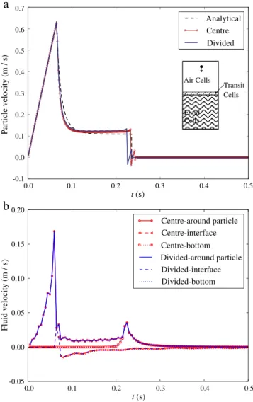
The predictions are compared inFig. 2against the analytical solu-tion. Also compared in thefigure are the two methods on calculating the void fraction of thefluid cell. It is evident fromFig. 3a that the pre-dicted settling velocities of the particle by both methods agree well with the analytical solution. The numerical predictions capture well the sharp reduction of velocity when the particle hits the water and bounces back when it hits the container bottom. The settling process
in the water also compares well with the analytical solution. Interest-ingly, the centre void fraction method appears to perform slightly better than the divided method. This may have been caused by the use of identical cell size with the particle diameter. However, a rather different scenario is observed in the next example.Fig. 2b presents thefluid cell velocity at three locations: around the particle, at the centre of the transition zone and at the bottom of the container (all along the centre line). As can be seen, the velocity of thefluid cell around the particle bears close correlation with the motion of the particle. The particle motion impacts the cell at the transitional interface only temporarily, and its interaction with the bottom cell is clearly observed before the particle hits the bottom.
3.2. One-dimensional consolidation
The proposed method has also been benchmarked by the classical one-dimensional (1D) consolidation problem in soil mechanics. A similar problem has been discussed by Suzuki et al. and Chen et al. [7,25]. According to the 1D consolidation theory by Terzaghi [26], the dissipation of excess pore pressure in a one-way drained soil
0.7 0.6 0.5 0.4 0.3 0.2 0.1 0.0 0.0 0.1 0.2 0.3 0.4 0.5 -0.1 Analytical Centre Divided Air Cells Transit Cells Fluid Cells t (s) 0.0 0.1 0.2 0.3 0.4 0.5 t (s) Particle velocity (m / s) Centre-around particle Centre-bottom Centre-interface Divided-around particle Divided-interface Divided-bottom 0.20 0.15 0.10 0.05 0.00 -0.05 Fluid velocity (m / s)
a
b
Fig. 2.Comparison of the CFD–DEM prediction and the analytical solution for single-particle settling in water with thecentreanddividedvoid fraction methods. (a) Particle velocity (inset: the settling problem and CFD mesh); (b) Fluid cell velocity at different locations: around the particle, the centre interface (transition) cell and the bottom centre cell.
2
layer subjected to surface surcharge can be described by the following equation: ∂p ∂t¼Cv ∂2 p ∂z2 ð12Þ
wherepdenotes the excess pore pressure during the consolidation,z is the vertical coordinate in the drainage direction, andCvis the
coef-ficient of consolidation given by
Cv¼
kp
ρwgmv ð
13Þ wherekpis the permeability,kp¼
d2ε3ρ
wg
150μð1−εÞ2[30].mvis the coefficient
of volume change,mv=Δεv/Δσv(ΔεvandΔσvare the variations of vertical strain and vertical stress, respectively) which can be deter-mined from the material properties and problem specification. In addition, a non-dimensional time can be defined to conveniently de-scribe the normalized time process[41]
Tv¼
Cvt
H2 ð14Þ
whereH is the height of the soil layer (its initial value being H0).
The initial and boundary conditions for the one-way drainage prob-lem are: p zð;0Þ ¼p0;pð0;tÞ ¼0;∂ p ∂z z¼H¼ 0: ð15Þ
The analytical solution to Eqs.(12)–(15)for the excess pore water pressure during the consolidation process is (see[10])
p¼X n¼∞ n¼1 2p0 nπð1−cosnπÞsin nπz H exp −n2π2 Tv 4 ! ð16Þ wherendenotes an integer number.
In simulating the one-dimensional consolidation problem, we con-sider a soil column comprised of 100 equal radius spheres (r=0.5mm) which are supposed to be saturated in water. The dimension of the column is 1 mm wide and 100 mm high, the same as that treated by Suzuki et al. and Chen et al.[7,25]. The column is discretized intofluid cells of 2 mm high each. Hooke contact law is adopted for the DEM com-putation, and the values of relevant parameters are adopted as the same in Suzuki et al.[25] (ρp=2650kg/m3, contact stiffnesskn=100N/m, ρf=998.2kg/m3,fluid viscosityμf=0.9982×10⁻³Pa-s, Gravity constant g=9.81m/s2). All particles are initially placed at the centre line of the column without any overlap and are emerged in water. The gravitational force and buoyancy force are then switched on to allow the particles to settle to a hydrostatic state (see also[7]). Once the initial consolidation isfinished, a surcharge loadp0=100Pa is then applied at the top of
the column.
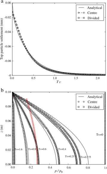
The simulated settlement of the top particle and the dissipation of excess pore water with time are compared inFig. 3against the analyt-ical solutions. The performances of the two void fraction calculation methods are also compared. As shown inFig. 3a, the predicted settle-ments of the top particle by both methods compare well with the analytical solution, except atTv= 0. Whilst the analytical solution as-sumes an instantaneous buildup of excess pore pressure throughout the column once the surcharge is applied, the CFD–DEM calculation needs certain time to build up the whole excess pore water. The numerical and analytical solutions hence are not totally comparable at the instant ofTv= 0. Following a similar strategy as suggested by Chen et al.[7], we have shifted the time measure of the numerical computation to certain small time to match the initial excess pore water pressure field for the analytical case, from which instant of time the two solutions are then compared. Nevertheless, it is suggested that the predicted quantities, including both the settlement and the excess pore water pressure, at the early stage of the consoli-dation remain less reliable due to the same reason. This explains the discrepancy between the numerical methods and the analytical solution for the dissipation of excess pore pressure in the case of Tv= 0.175 inFig. 3b (note that theTv= 0 case has been imposed by the initial conditions forp).
As shown inFig. 3b, except in the early stage and the case ofTv= 0.8, the predicted dissipations of excess pore pressure using both methods of void fraction calculation are in good agreement with the analytical solution. It is of particular interest to discuss the case of Tv= 0.8 inFig. 3b. The curve in red circle (see online) represents the predictions by the centre void fraction method. As compared to the analytical solution, the divided void fraction method evidently provides significantly better predictions than the centre void fraction method, which exemplifies the potential pitfall associated with the latter. A further inspection of the results reveals that the initial con-solidation (driven by gravitational force and buoyancy force) has resulted in a settlement around 0.4 mm for some particles on the top. AtTv= 0.8 of the normal consolidation stage, there is an extra settlement around 0.09 mm occurring for these particles. The total
a
b
Analytical Centre Divided Analytical Centre Divided 0.0 0.5 1.0 1.5 2.0 T 0.00 -0.02 -0.04 -0.06 -0.08 -0 T op particle settlement (mm) 0.0 0.2 0.4 0.6 0.8 1.0 Tv=0 Tv=1.6 Tv=0.8 Tv=0.6 Tv=0.4 Tv=0.25 Tv=0.175 0.10 0.08 0.06 0.04 0.02 0.00 p / p0 z (m)Fig. 3.Benchmarking of CFD–DEM simulations of the consolidation settlement and the dissipation of excess pore pressure with the classic Terzaghi's analytical solution to the 1D consolidation problem. Centre: centre void ratio method; Divided: divided void ratio method. (For interpretation of the references to colour in thisfigure legend, the reader is referred to the web version of this article.)
settlement of such particles thus reaches around 0.5 mm, which may exactly lead to a situation that the centre of the concerned particle comes across the boundary of two neighbouring cells (similar to the case of Particle E in Fig. 1). According to the centre void fraction method, there will be a sudden jump of void fraction for neighbouring cells and hence the drag forces as well, which may lead to the ob-served erroneous results shown inFig. 3b. Whilst the divided void fraction method offers improved accuracy, the centre void fraction method is advantageous in terms of efficiency, especially when the simulated system is extremely large. Evidently, if the particle size is very small relative to thefluid cell, the difference in predictions be-tween the two void fraction methods is expected to become small.
The overall performance of the CFD–DEM program has been found satisfactory with the above two benchmarking examples. Thefluid– particle interaction appears to be reasonably captured. The numerical algorithms solving the governing equations of both the CFD and the DEM parts are generally stable and robust.
4. Application to conical sandpiling in water
Handling and processing of granular materials are commonplace in many engineering branches and industries. The piling of granular media, for example, has been common in open stockpiles in agricul-ture, chemical engineering and mining industries. The angle of repose and the stress distribution in a sand pile have been the focus of DEM studies on sand pile formation (see[38]on a review of this topic). In particular, the pressure minimum in the vertical stress profile of the base of a sand pile has been an interesting phenomenon attracting
much attention in classic granular mechanics. The occurrence of pres-sure dip can be caused by many factors, e.g., the base deflection[36], the particle shape [34,40] and the construction methods [4,29]. Appreciable pressure dip has been observed in a sand pile prepared by localizedflow source such as hopper, whilst using raining sieve produces a sand pile with a central peak normal stress. Whilst a dom-inant body of existing studies on sandpiling has been focused on the case of dry granular materials, research on sandpile formation in an environment of water is scarce. The latter case mayfind rather inter-esting applications in practice, ranging from silos to road and dam constructions, land reclamation and dredging, mine product and tail-ing handltail-ing as well as soil erosion and debrisflow. A deeper under-standing towards the fundamental principles governing the stress transmission in static granular solids submerged in water may lead to not only considerable advances in the theory of granular mechan-ics but also improved technologies for relevant practical applications mentioned above. The CFD–DEM method developed above will be employed in this paper to examine the behaviour of sandpiling in water. Particles are poured from a hopper through a containerfilled with water to form conical sand piles on a circularflat panel placed at the bottom of the container (seeFig. 4). To ensure proper conical sandpiles can be formed, the circular panel is limited by a round baffle with 2 mm high (similar to way employed in the tests by[17]). The particlesflowing beyond the baffle will drop off and will be removed from consideration. Meanwhile the corresponding cases without the presence of water (hereafter referred to as thedrycases) will also be simulated for comparison.
Whilst the particle shape is found affecting the characteristics of the pressure dip in a sandpile (see[2,34,35,40]), it is considered ap-proximately here by considering the rolling resistance among spher-ical particles. Following the model by Zhou et al.[35], one has
Mr¼−μrFnRr ωrel
ωrel
j j ð17Þ
whereMris the torque between two contacted particles.Fnis the con-tact normal force.Rris the rolling radius defined byRr=rirj/(ri+rj) whereriandrjare the radii of the two spherical particles in contact. μris the coefficient of rolling resistance. Zhou et al. and Zhou and Ooi[34,35]have emphasized the importance of rolling friction in achieving physically/numerically stable sandpiles. To highlight its role in the wet case, a comparative study of two rolling resistance cases,μr= 0 andμr= 0.1, is conducted. Note that a small baffle used for the ground panel is especially useful to ensure the forming of proper sandpiles in the case of free rolling (μr= 0). In addition, we have examined both monosized and polydisperse grain size distribu-tion. The polydisperse packing follows a typical grain size distribution of sand. To render the two cases comparable, the mean grain size of the polydisperse packing is chosen to be equal to the particle size of the monosized case.Table 1summarizes the relevant parameters used in the subsequent computation.
We simulate a real case of forming a sand pile in 10 s, among which around 6 s is spent in pouring all particles through the hopper into the water and onto the circular panel and around 4 s for the relaxation of all particles (some may fall off the receiving panel) until theyfinally settle down (with an overall kinetic energy reaching a magnitude around 10−14J). Because very small time steps have
been used in both the DEM and CFD computations to solve the prob-lem, adequate accuracy can be achieved by stepping 1000 DEM calcu-lations after one step of CFD computation. The total computing time for each realization of sandpile in water, on a 4-core Intel CPU (3.0 GHz) desktop computer, is around 2 days. Thefinal stable-state sandpile will be used to extract such information as stress distribu-tion, repose angle, void ratio distribution and contact force chains for the subsequent analysis. In particular, both the centre and divided void fraction methods have been used for the problem. Only marginal
Fig. 4.Illustration of the formation of a sand pile through hopperflow in water: (a) during the formation of the sandpile; (b) thefinal state of the sandpile.
difference has found between the predictions by the two methods. Hence only the simulations by the divided void fraction method will be presented in the subsequent sections.
4.1. Repose angle
The repose angleϕof sandpile formed in water (referred in the sequel as“wet case”) has been compared to that for the dry case, for both monosized and polydisperse packings. In measuring the re-pose angle, the position of each particle is projected onto the plane ofr−z whererdenotes its horizontal distance to the axis of the pile (assumed to be identical to the axis of the hopper). The peak of all sandpiles obtained in our study has been found ratherflat with a vertical heightHslightly less than the conical apexHaas shown in Fig. 6. The apex heightHawill be used to normalize the vertical pres-sure profile. The obtained results are summarized inTable 2for the case ofμ= 0.7.
It is observed fromTable 2that, for themonosized casewithout consideration of rolling resistance, the repose angle for a sandpile formed in water is fairly close to that in the dry case. However, if the rolling resistance is considered, it becomes considerably smaller than that in the dry case. From our simulation the difference is found to be around 9∘. However, the observation is quite different for
thepolydisperse case, where the obtained repose angle in the dry case
differs only around 1∘from the wet case. Its value in dry case is slightly greater than the wet case for the free rolling case (μr= 0), but is margin-ally smaller than the latter in consideration of rolling resistance. In any of these cases, considering rolling resistance leads to appreciably in-creased repose angle for a sandpile than otherwise. This is consistent with the observation by Zhou and Ooi[34]. Meanwhile, our study indi-cates that there is a mixed effect of the polydispersity of a packing on the obtained sandpile. Without consideration of rolling resistance, the monosized and polydisperse packings produce roughly the same repose angle. When the rolling resistance is considered, a much smaller repose angle is found for a dry polydisperse packing than a dry monosized case, whereas it is greater in the wet polydisperse case than in the wet monosized case.
4.2. Pressure dip
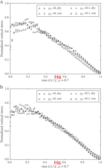
Fig. 7depicts the vertical pressure profiles at the base of sandpiles obtained from our simulations. Clear pressure dip at the centre is found for all cases.Table 2also presents the specific values of the normalized dip and peak pressures. In particular, the effects of the following factors on the observed pressure dip can be identified
(a)Water. A sandpile formed in water generally has aflatter dip
(a smaller relative pressure dip) than the dry case. The differ-ence in the relative pressure dip can be two times as much.
(b) Rolling resistance. Under otherwise identical conditions, the
consideration of rolling resistance may lead to an increase in the relative pressure dip for monosized packings, but a moderate decrease for the polydisperse case.
(c)Polydispersity. A polydisperse sample generally leads to a smaller
relative pressure dip than a monosized one. 4.3. Void ratio
It is interesting to explore the features of both average void ratio and the local void ratio in each sandpile. We employ the Voronoi
Table 1
Physical and geometric parameters used in the sandpiling simulations.
Characteristics of the packings Monosized 15,000 particles, 2 mm in diameter.
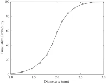
Polydisperse 15,000 particles, diameter ranged from 1 to 3 mm
(mean=2 mm, the cumulative grain size distribution shown inFig. 5)
Particle and contact parameters Particle density 2700 kg/m3
Interparticle friction coefficienta μ
= 0.7 Young's modulus
(Hertz model)
70 GPa (particle–particle contact) 700 GPa (particle–wall contact)
Poisson's ratio 0.3
Restitution coefficienta 0.7
Rolling friction (using the torque model of[35]) μr= 0 & 0.1
Geometry of the hopper & the circular panel
Hopper diameter 14 mm
Hopper height (from the hopper bottom to the receiving panel) 40 mm
Radius of the receiving panel 5 cm
Baffle height 2 mm
Simulation control Time step (DEM) 5 × 10⁻⁷s
Time step (CFD) 5 × 10⁻⁴s
Simulated real time 10 s (20,000,000 steps in DEM)
a
Note that in practice, different values for both the coefficient of interparticle friction and the coefficient of restitution should be used for the in air and in water cases, i.e., according to Malone and Xu[19]. For simplicity, they are kept the same in both cases in this study to highlight the pure effect of water presence (e.g., interaction forces).
100 80 60 40 20 0 1.0 1.5 2.0 2.5 3.0 Diameter d (mm) Cumulative Probability
Fig. 5.Cumulative grain size distribution of the polydisperse packing used for sandpiling
tessellation of a sandpile to calculate these quantities. Shown in Fig. 8a are the Voronoi tessellation cells for a typical sandpile. Since each Voronoi cell is occupied by a single particle, the local void ratio can be conveniently determined. Based on the local void ratio, the average void ratio can also be obtained. In calculating the void ratios, particles/cells in the bottom layers which are below the height of the baffle have been excluded for consideration.
Table 2
Comparison of the characteristics of sandpiles obtained for the dry/wet cases and monosized and polydisperse packings (interparticle friction coefficientμ= 0.7).
Sandpile characteristics Monosized packing Polydisperse packing
μr= 0 μr= 0.1 μr= 0 μr= 0.1
Dry Wet Dry Wet Dry Wet Dry Wet
Repose angleϕ(o
) 22.4 20.6 31.5 22.6 23.3 20.6 27.4 26.0
Final particle number in the sandpile 13,348 13,138 11,604 9476 14,681 15,000 14,328 14,989
Normalized dip stress 0.3865 0.661 0.345 0.668 0.572 0.81 0.63 0.719
Normalized peak stress (bygHa) 0.654 0.724 0.721 0.776 0.869 0.93 0.87 0.878
Relative pressure dipa
(%) 40.90 8.70 52.15 13.92 34.18 12.90 27.59 18.11
Average void ratio 1.243 1.27 1.376 1.397 1.459 1.481 1.545 1.571
Fabric Anisotropy 0.2717 0.2368 0.4988 0.3919 0.0516 0.0839 0.1825 0.1853
a
Relative pressure dip = (peak stress−dip stress) / peak stress.
1.0 0.8 0.6 0.4 0.2 0.0 1.0 0.8 0.6 0.4 0.2 0.0 1.0 0.8 0.6 0.4 0.2 0.0 1.0 0.8 0.6 0.4 0.2 0.0 r r=0, dry =0, wet r r=0.1, dry =0.1, wet r r=0, dry =0, wet r r=0.1, dry =0.1, wet rtan ( ) / z , = 0.7 rtan ( ) / z , = 0.7
Normalized vertical stress
Normalized vertical stress
a
b
Fig. 7.Profile of vertical pressure at the base of sand piles for (a) monosized packings and (b) polydisperse packings. dry- r = 0 wet- r = 0.1 wet- r = 0 dry- r = 0.1 dry- r = 0 wet- r = 0.1 wet- r = 0 dry- r = 0.1 0.8 1.0 1.2 1.4 1.6 1.8 2.0 1.0 1.5 2.0 2.5 3.0 void ratio,e void ratio,e 3.5 3.0 2.5 2.0 1.5 1.0 0.5 0.0 1.0 0.8 0.6 0.4 0.2 0.0 Probability Probability
b
a
c
Fig. 8.(a) Voronoi tessellation of a sandpile; (b) comparison of the local void ratio distri-bution for monosized packings; (c) local void ratio distridistri-bution for polydisperse packings. In both (b) and (c), the symbols are numerical data, and the dash or solid lines arefittings by Gamma distribution.
Ha
As shown inTable 2, the presence of water leads to a slightly increased void ratio as compared to the dry case. The consideration of rolling resistance and polydispersity, however, may result in signif-icantly looser sandpile than otherwise. Shown inFig. 8are the local void ratio distributions andfittings for both the monosized and poly-disperse cases. As can be seen, a Gamma distributionfits much better for the monosized cases (regardless dry or wet, considering rolling resistance or not) than for the polydisperse cases. In each of the monosized cases, a bestfit Gamma distribution slightly underesti-mates the peak probability of the local void ratio. In the polydisperse cases, the optimal Gamma distribution provides systematically over-estimation in the small void ratio region and underover-estimation in the tail part, but nevertheless captures the peak well. The polydisperse case reaches a peak probability at a slightly smaller void ratio than the corresponding monosized case. In all cases, the presence of water or considering rolling resistance may lead to the peak void ratio shifted rightwards to a bigger value. Such an effect caused by the consideration of rolling resistance is more obvious than by the presence of water.
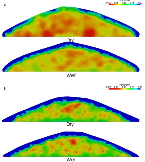
Meanwhile, we have further visualized the distribution of local void ratio in a sandpile inFig. 9. In the monosized case as shown inFig. 9a, two clear dense areas are observed in the dry sandpile which serve as the anchoring points for an arch to be formed around the sandpile centre and induce the observed pressure dip. In the wet case the distri-bution of void ratio at the bottom has been much smoothed and no particular denser areas are present. In the polydisperse case, the pres-ence of water appears to have rather limited impact on the local void
distribution where similar local void ratio distributions are found in both the dry and the wet cases.
4.4. Fabric structure and fabric anisotropy
Indicative information of pressure dip can be obtained from the contact force network (or fabric) of a sandpile[5,18,23], which is shown inFig. 10for theμr= 0 case in the present study. In the dry monosized case (Fig. 10a upper panel), the strong force chains show an appreciable orientation with an inward inclination angle of around 70∘. This indicates that the weights of the upper particles of the sand-pile are transferred to the bottom along these inclined chains rather than along the vertical direction. The bottom centre part of the sand-pile is shielded from supporting the weights, which explains the strong pressure dip observed in this case. In contrast, in the wet monosized case (Fig. 10a bottom panel), the contact force chains are more preferably oriented to the vertical direction, and no effective shield can be formed to deflect the upper weights. A much reduced pressure dip is naturally found for this wet case. The observation dif-fers for the polydisperse cases shown inFig. 10b. The polydispersity appears to totally change the force transmission pattern, as has been noticed by Luding[18]as well. In both the dry and wet cases, the strong force chains are more vertically oriented, and result in re-duced pressure dip in these cases. Moreover, for both monosized and polydisperse cases, the presence of water renders the entire contact force network more homogeneous than in the dry case, and the
Fig. 9.Comparison of the local void ratio contour (μr= 0). (a) The monosized case, (b) the polydisperse case. In each case, the upperfigure corresponds to the dry packing and the
greatest contact forces are larger in the dry case than in the wet case. Not presented here, the consideration of rolling resistance renders the force chains more vertically oriented, in a similar manner as the effect of polydispersity.
Evidently, the fabric structure inFig. 10is not isotropic, and the degree of fabric anisotropy in these contact networks can indeed be quantified. To this end, we employ a interparticle-contact-based fab-ric tensor proposed by Satake[22] and use its second invariant to quantify the degree of fabric anisotropy in a sandpile (see[14]on a similar way of using the fabric tensor and its invariant). The results are summarized inTable 2. As is shown, the fabric anisotropy is mod-erately reduced in the presence of water for monosized samples, whereas the opposite trend is observed in the polydisperse case. The consideration of rolling resistance generally leads to significant increase of fabric anisotropy, whereas the polydispersity results in reduced fabric anisotropy. A positive correlation is observed between the fabric anisotropy and pressure dip ratio for the monosized cases. No apparent correlation can be found for the polydisperse cases. 5. Concluding remarks
A coupled CFD–DEM method has been presented to simulate the interaction betweenfluid and particles in granular media. In the meth-od, we employ the DEM to simulate the motion and interactions of
particles for a granular particle system, and use the CFD to solve the lo-cally averaged Navier–Stokes equation forfluidflow. The interaction between fluid and particle is considered by exchanging such interaction forces as drag force and buoyancy force between the DEM and the CFD. Through two benchmarking examples and another appli-cation to the formation of sandpile in water, the following conclusions can be made:
• The proposed method is adequately robust and efficient to be applied to the simulation offluid–particle interaction for a wide variety of problems in geomechanics.
• The behaviour offluid–particle interaction in granular media can be reasonably captured by the proposed method, as has been demon-strated by benchmarking with the single particle settling in water problem and the one-dimensional consolidation problem.
• Based on the CFD–DEM simulation of the conical sandpile problem, it is observed that, (a) the presence of water may help to form a sand-pile with more homogeneous internal structures in terms of local void ratio, contact force network and fabric anisotropy. It may also help to reduce the relative pressure dip; (b) considering the rolling resistance among particles may lead to a greater relative pressure dip for the monosized case and a smaller one for the polydisperse case. The observation holds for both dry and wet cases; (c) a sandpile formed by using polydisperse granular material may have a smaller
relative pressure dip than using a monosized material; and (d) the local void ratio in a sandpile with monosized particles yields Gamma distribution. The characteristic is not so obvious for a sandpile formed by polydisperse particles.
The observations made above still need rigorous verifications by experiments in the future. The study nevertheless constitutes afirst step towards effective modelling the complex interaction between
fluids and particles in porous media such as sand. Further improve-ments may be made by considering more realistic particle shape and more reasonable interaction forces in the coupling analysis. Whilst it has been developed for applications relevant to geotechnical engineer-ing, the proposed approach can be equally useful for problems in other
fields such as mining and chemical engineering where thefluid–particle interaction is considered important.
Acknowledgement
The study was supported by the Research Grants Council of Hong Kong (RGC/GRF 623609).
References
[1] J. Ai, Particle scale and bulk scale investigation of granular piles and silos, Ph.D. thesis, The University of Edinburgh, 2010.
[2] J. Ai, J.F. Chen, J.M. Rotter, J.Y. Ooi, Assessment of rolling resistance models in discrete element simulations, Powder Technology 206 (2011) 269–282.
[3] T.B. Anderson, R. Jackson, Fluid mechanical description offluidized beds. Equa-tions of motion, Industrial and Engineering Chemistry Fundamentals 6 (1967) 527–539.
[4] B. Brockbank, J.M. Huntley, R.C. Ball, Contact force distribution beneath a three dimensional granular pile, Journal de Physique II France 7 (1997) 1521–1532. [5] M.E. Cates, J.P. Wittmer, J.-P. Bouchaud, P. Claudin, Jamming, force chains, and
fragile matter, Physical Review Letters 81 (1998) 1841–1844.
[6] F. Chen, Coupledflow discrete element method application in granular porous media using open source codes, Ph.D. thesis. University of Tennessee, 2009. [7] F. Chen, Eric C. Drummb, G. Guiochon, Coupled discrete element andfinite volume
solution of two classical soil mechanics problems, Computers and Geotechnics 38 (5) (2011) 638–647.
[8] F. Concha, Settling velocities of particulate systems, KONA Powder and Particle Journal 27 (2009) 18–37.
[9] P.A. Cundall, O. Strack, A discrete numerical model for granular assemblies, Geotechnique 29 (1979) 47–65.
[10] B.M. Das, Advanced Soil Mechanics, Hemisphere Publishing Corporation and McGraw-Hill, 1983.
[11] R. Di Felice, The voidage function forfluid–particle interaction systems, International Journal of Multiphase Flow 20 (1994) 153–159.
[12] C. Goldenberg, I. Goldhirsch, Friction enhances elasticity in granular solids, Nature 435 (2005) 188–191.
[13] C. Goniva, C. Kloss, A. Hager, S. Pirker, An open source CFD–DEM perspective, Proc. of the 5th OpenFOAM Workshop, June 22-24 2010, (Göteborg). [14] N. Guo, J. Zhao, The signature of shear-induced anisotropy in granular media,
Computers and Geotechnics 47 (2013) 1–15.
[15] K.D. Kafui, C. Thornton, M.J. Adams, Discrete particle–continuumfluid modelling of gas–solidfluidised beds, Chemical Engineering Science 57 (2002) 2395–2410.
[16] C. Kloss, C. Goniva, LIGGGHTS: a new open source discrete element simulation software, Proc. 5th Int. Conf. on Discrete Element Methods, London, UK, August 2010, (website:www.liggghts.com).
[17] Y.J. Li, Y. Xu, C. Thornton, A comparison of discrete element simulations and ex-periments for‘sandpiles’composed of spherical particles, Powder Technology 160 (2005) 219–228.
[18] S. Luding, Stress distribution in static two-dimensional granular model media in the absence of friction, Physical Review E 55 (4) (1997) 4720.
[19] K.F. Malone, B.H. Xu, Particle-scale simulation of heat transfer in liquid-fluidised beds, Powder Technology 184 (2008) 189–204.
[20] R.L. Michalowski, N. Park, Admissible stressfields and arching in piles of sand, Geotechnique 54 (2004) 529–538.
[21] C. O'Sullivan, Particulate Discrete Element Modelling: A Geomechanics Perspective, Spon Press (an imprint of Taylor & Francis), London, 2011.
[22] M. Satake, Fabric tensor in granular materials, in: P.A. Vermeer, H.J. Luger (Eds.), Deformation and Failure of Granular Materials, Balkema, Rotterdam, 1982, pp. 63–68. [23] J.H. Snoeijer, T.J.H. Vlugt, M. van Hecke, W. van Saarloos, Force network ensemble: a new approach to static granular matter, Physical Review Letters 92 (5) (2004) 054302.
[24] G.G. Stokes, On the theories of internal friction offluids in motion and of the equi-librium and motion of elastic solids, Transactions Cambridge Philological Society 8 (9) (1844) 287–319.
[25] K. Suzuki, et al., Simulation of upward seepageflow in a single column of spheres using discrete-element method withfluid–particle interaction, Journal of Geotechnical and Geoenvironmental Engineering 133 (1) (2007) 104–110.
[26] K. Terzaghi, Theoretical Soil Mechanics, Wiley, New York, 1943.
[27] Y. Tsuji, T. Kawaguchi, T. Tanaka, Discrete particle simulation of two-dimensional
fluidized bed, Powder Technology 77 (1993) 79–87.
[28] Y. Tsuji, T. Tanaka, T. Ishida, Lagrangian numerical simulation of plugflow of co-hesionless particles in a horizontal pipe, Powder Technology 71 (1992) 239–250. [29] L. Vanel, Howell D., J. Clark, R.P. Behringer, E. Clément, Effects of the construction history on the stress distribution under a sand-pile.lanl eprint, cond-mat/9906321, 1999.
[30] L.M. Warren, C.S. Julian, H. Peter, Unit Operations of Chemical Engineering, 7th edition, McGraw-Hill, New York, 2005, pp. 163–165.
[31] J.P. Wittmer, P. Claudin, M.E. Cates, J.P. Bouchaud, An explanation for the central stress minimum in sand piles, Nature 382 (1996) 336–338.
[32] B.H. Xu, Y.Q. Feng, A.B. Yu, S.J. Chew, P. Zulli, A numerical and experimental study of gas–solidflow in afluid-bed reactor, Powder Handling and Processing 13 (2001) 71–76.
[33] B.H. Xu, A.B. Yu, Numerical simulation of the gas–solidflow in afluidized bed by combining discrete particle method with computationalfluid dynamics, Chemical Engineering Science 52 (1997) 2785–2809.
[34] C. Zhou, J.Y. Ooi, Numerical investigation of progressive development of granular pile with spherical and non-spherical particles, Mechanics of Materials 41 (2009) 707–714.
[35] Y.C. Zhou, B.D. Wright, R.Y. Yang, B.H. Xu, A.B. Yu, Rolling friction in the dynamic simulation of sandpile formation, Physica A 269 (1999) 536–553.
[36] Y.C. Zhou, B.H. Xu, R.P. Zou, A.B. Yu, P. Zulli, Stress distribution in a sandpile formed on a deflected base, Advanced Powder Technology 14 (2003) 401–410. [37] H.P. Zhu, Z.Y. Zhou, R.Y. Yang, A.B. Yu, Discrete particle simulation of particulate
systems: theoretical developments, Chemical Engineering Science 62 (2007) 3378–3396.
[38] H.P. Zhu, Z.Y. Zhou, R.Y. Yang, A.B. Yu, Discrete particle simulation of particulate systems: a review of major applications and findings, Chemical Engineering Science 63 (2008) 5728–5770.
[39] I. Zuriguel, T. Mullin, J.M. Rotter, The effect of particle shape on the stress dip under a sandpile, Physical Review Letters 98 (2007) 028001.
[40] I. Zuriguel, T. Mullin, The role of particle shape on the stress distribution in a sandpile, Proceedings of the Royal Society of London, Series A 464 (2008). [41] T.W. Lambe, R.V. Whitman, Soil Mechanics, Wiley, New York, 1969.