Visualisation of heterogeneous data with simultaneous
feature saliency using Generalised Generative
Topographic Mapping
Shahzad Mumtaz, Michel F. Randrianandrasana, Gurjinder Bassi and Ian T. Nabney System Analytics Research Institute (SARI),
Aston University, Birmingham, B4 7ET, United Kingdom.
Email: mumtazs;randrimf;t-bassig;[email protected]
Abstract. Most machine-learning algorithms are designed for datasets with fea-tures of a single type whereas very little attention has been given to datasets with mixed-type features. We recently proposed a model to handle mixed types with a probabilistic latent variable formalism. This proposed model describes the data by type-specific distributions that are conditionally independent given the latent space and is called generalised generative topographic mapping (GGTM). It has often been observed that visualisations of high-dimensional datasets can be poor in the presence of noisy features. In this paper we therefore propose to extend the GGTM to estimate feature saliency values (GGTMFS) as an integrated part of the parameter learning process with anexpectation-maximisation(EM) algo-rithm. The efficacy of the proposed GGTMFS model is demonstrated both for synthetic and real datasets.
1
Introduction
Type-specific data analysis has been well studied in the machine learning commu-nity [6]. In the recent couple of decades, the need to analyse mixed-type data is gaining a lot of attention from machine learning experts because of the fact that real world processes often generate a data of mixed-type. An example of such a mixed-type data could be a hospital’s patients’ dataset where typical fields include age (discrete or con-tinuous), gender (binary), test results (binary or concon-tinuous), height (continuous) etc. In practice a number of ad-hoc solutions are used to handle mixed-type data [6]. However, the ideal general solution for analysing such heterogeneous data is to specify a model that builds a joint distribution with the assumption of an appropriate noise distribution for each type of feature set (for example a Bernoulli for modelling binary, a multino-mial for modelling multi-category features and a Gaussian for modelling continuous features) and then fitting the model to data where the parameter estimates are used to draw inferences [6].
In the literature there is no multivariate distribution that can model random vari-ables of different types. However, one possible way of jointly modelling discrete and continuous features is using a latent variable approach to understand the correlation be-tween features of different types in combination. Type-specific latent variable models have already been proposed such as a generative topographic mapping (GTM) appro-priate for continuous features and a latent trait model (LTM) approappro-priate for discrete
type features [7] (an LTM was proposed as a generalisation of GTM model). This has encouraged us to recently propose to combine GTM and LTM [13] in a probabilistic non-linear latent variable model in a principled way to visualise mixed-type data on a single continuous latent space under a unified proposed framework of conditional inde-pendence criteria: we called this model a generalised-GTM (GGTM).
In principle, the machine learning algorithms assume to perform well in cases where we have more information about data instances. This suggests that the use of more features is important for the learning algorithms. However, in practice it is observed that not all the features are important. It is therefore useful to select a subset of features which are relevant thereby ignoring the irrelevant (noisy) features which compromise performance of the learning algorithm [8,9]. An understanding of which features are relevant is valuable in its own right. In the exploratory phases of analysis (which is when data visualisation is most used) it is usual to measure as many variables as is feasible, since it is not known which features are relevant to the task. Feature selection then plays an important role in simplifying the task and making data collection cheaper and faster.
Feature selection (FS) has been widely used in supervised learning problems where the search is guided by the known target values. FS methods can be categorized into four classes [1,14]: filters, wrappers, hybrid and embedded. Details of each of them are given in [10,14]. FS for unsupervised learning algorithms is a challenging task as there are no target values to guide the search. Very few attempts have been made to estimate the importance of features in the unsupervised learning algorithms. A brief review of feature selection in a clustering perspective is given in [1,4,8,14,18] and details of some previous attempts in the latent variable formalism are given in [5,9,11,15,16,17]. To the best of our knowledge, there is no similar approach in the literature for estimating fea-ture saliency when modelling mixed-type data, though [4] did discuss this as a possible extension in the clustering perspective.
Our focus in this paper is to demonstrate an extension of the GGTM model to esti-mate feature saliency values not only for discrete type features but also for mixed-type features in a dataset, as an integrated part of the parameter learning process, under the latent variable formalism. The structure of the remainder of the paper is as follows. In Section 2, we explain our proposed GGTMFS model and derive the EM parameter learning process. Section 3 describes our experiments to demonstrate the effectiveness of the proposed approach. We conclude the paper in Section 4.
2
A GGTM with Simultaneous Feature Saliency (GGTMFS)
The main goal of a latent variable model is to find an M-dimensional manifold,H, (usuallyM = 2) for the distributionp(x)in a high-dimensional data space,D, withD -dimensions. We write each observation vector,xnin terms of sub-vectorsxRn,xBn and xCn for continuous, binary and multi-category features respectively. In the rest of this paper we use superscriptRfor continuous features, superscriptBfor binary features and superscriptCfor categorical features. The symbol|.|is used to indicate the number of features in each type of data space. We also useMto indicate eitherRorBorC.
In this paper, we now propose an extension of the GGTM visualisation model de-scribed in [10] to simultaneously estimate feature saliencies (we call this extension GGTMFS) and learn the model parameters. To estimate feature saliency values, we assume that each feature is independent of the component label under the appropriate noise model distribution. As a special case for the Gaussian noise model, the feature in-dependence assumption is modelled by adopting diagonal covariance matrices (as used in [8,9]) instead of spherical covariance (as used in [3] and GGTM). Now the probabil-ity densprobabil-ity function of the GGTMFS model takes the form
p(xn|π, Θ) = K X k=1 πk Y M |M| Y d=1 p(xMnd|ΘMkd) , (1)
wherep(.|ΘMkd)is the probability density functions of thedth feature for thekth com-ponent andπkis the mixing coefficient of thekth component and is taken to be fixed to
1
K for all the components in the mixture model andM ∈ {R,B,C}) indicates type of data space (and the corresponding distributional assumption).
We make the definition thatΨM = (ψ1M,· · · , ψM|M|)(whereM ∈ {R,B,C}), is the set of binary indicators ψdM = 1 for a relevant feature andψMd = 0otherwise. Combining ψM
d for each type of variable, we obtain Ψ = {ΨR, ΨB, ΨC}. Now the probability density of our mixture model takes the form
p(xn|π, Θ, λ, Ψ) = K X k=1 πk Y M |M| Y d=1 [p(xMnd|ΘkdM)]ψdM[q(xM nd|λMd )] (1−ψMd ) . (2)
The common distributionq(xMnd|λMd )is designed to explain all the data that is poorly explained by the GGTM model. The notion of feature saliency is modelled as follows: we first treatψdMas a missing variable in the EM algorithm and as a second step we estimate the feature saliency,ρMd =p(ψdM= 1), which is the probability that thedth feature is relevant. The resulting model now takes the form,
p(xn|Ω) = K X k=1 πk Y M |M| Y d=1 [ρMd p(xMnd|ΘkdM)] + [(1−ρMd )q(xMnd|λMd )] , (3) whereΩ=nπk, ΘMkd , λMd ,
ρMd ois the set of all the parameters of the model. A simple way to understand how Equation (3) is obtained is to observe that[p(xMnd|ΘkdM)]ψdM
[q(xMnd|λdM)]1−ψdM can be re-written asψM d [p(x M nd|Θ M kd)] + (1−ψ M d )[q(x M nd|λ M d )] given thatψMd is a binary indicator variable (see the proof in [10,12]). The log-likelihood now takes the form
L(Ω) =
N X
n=1
2.1 An EM algorithm for GGTMFS
The latent structure of the GGTM model can be exploited to estimate feature saliencies, in a similar way as previously exploited for the standard GTM [9]. For this purpose, we consider flipping of a biased coin with probabilityρMd ; if the coin is a head then the feature is generated from the mixture component,p(.|ΘMkd), otherwise the ‘background component’ ,q(.|λMd ), is responsible.
We treatY(i.e. component labels) andΨ as missing variables and we can derive an EM algorithm for estimating model parameters (see details in [10,12]). In the E-step, we use the current set of parameters,Ω, to compute the posterior probability (i.e. responsibility)rnk=p(yn =k|xn)using Bayes’ theorem,
πk Q M h Q|M| d=1[ρMd p(xMnd|ΘkdM)] + [(1−ρMd )q(xMnd|λMd )] i PK k=1πk Q M h Q|M| d=1[ρMd p(xMnd|ΘMkd)] + [(1−ρMd )q(xMnd|λMd )] i. (5)
The responsibility matrix,R, is used to computeuMnkd = p(ψdM = 1, yn = k|xMn ), which is a measure of the importance of thenth data point relating to thekth component using thedth feature of theMtype observation space andvnkdM =p(ψMd = 0, yn =
k|xM n ). uMnkd= ρ M d p(x M nd|Θ M kd) ρMd p(xMnd|ΘkdM)] + [(1−ρMd )q(xnd|λMd )rnk, (6) vMnkd=rnk−uMnkd. (7) M-step:We can useUMto re-estimate the weight matrixWM(i.e.Mindicate type of observation space) using a set of linear equations. Both for binary and multinomial cases we use gradient-based approach as used in [7]. The weight vectorwMd of each
dth feature can be updated using
d wdR= (ΦTERdΦ)−1ΦTURdxRd, (8) ∆wBd ∝ΦThUBdxBd −EBdgB(ΦwBd)i, (9) ∆WCS d∝Φ ThUC dXCSd−E C dgC(ΦWCSd) i , (10)
whereΦis aK×Lmatrix,UdMis aK×N matrix calculated using Equation (6),xMd is anN×1data vector of real/binary values (theXCS
dis binary encoded matrix ofdth multi-category feature) and the diagonal matrixEMd has valueseMkkd=PNn=1uMnkd.
Now we can straightforwardly re-estimate parameters of the mixture model using the re-estimated weight matrix of each type,WcM: first we re-estimate the centres (for each type features) of the mixture model in the data space (see Equations (11), (12) and (13))
\
M eanΘkR=mdR
d
mBk =gB(Φ(zk)WdB), (12) \mCkS d=g
C(Φ(zk)wC
Sd), (13)
wheremdMk is a1× |M|vector,gB(.)is a logistic sigmoid andgC(.)is asoftmax func-tion. We use re-estimated centre to update the diagonal Gaussian width in each direction (for each continuous feature): see Equation (14) (similar to standard GTMFS [9])
1 c βdR = P k P nu R nkd(xRnd−mdRkd) 2 P k P nu R nkd . (14)
Common density parameters,λRd, can be updated using
\ M eanλR d = P n( P kv R nkd)xRnd P nkv R nkd . (15) \ M eanλBd = P n( P kv B nkd)x B nd P nkvnkdB . (16) M eanλ\C Sd= P n( P kv C nkd)x C nSd P nkvnkdC . (17) \ V arλRd = P n( P kvnkdR (xRnd−M eanλ\Rd) 2 P nkvnkdR . (18)
For the feature saliency parameter update, we use prior distributions for each type of variable separately as explained in [12]. The resultant feature saliency updates are
c ρRd = max( P nku R nkd− KP 2 ,0) max(P nkuRnkd− KP 2 ,0) + max( P nkvnkdR − T 2,0) , (19)
whereP andT are the number of parameters inΘkdR andλRd respectively.
c ρBd = max( P nku B nkd+αd−1,0) max(P nkuBnkd+αd−1,0) + max(PnkvBnkd+βd−1,0) . (20) c ρCd = maxP nku C nkd− K(cd−1) 2 ,0 maxP nk, uCnkd− K(cd−1) 2 ,0 + maxP nkvnkdC − (cd−1) 2 ,0 , (21)
wherecdrepresents number of categories for thedth feature. We also extend GGTMFS by deriving an expectation-maximisation(EM) variant to incorporate missing values (for details see the technical report [12]).
3
Experiments
A series of experiments was performed to demonstrate the effectiveness of the proposed GGTMFS model for both synthetic and real datasets. Each weight sub-matrix (i.e.WR, WBandWC) was initialised using principal component analysis (PCA). On average,
500iterations of EM were sufficient for convergence. We used a latent grid of size8×8
3.1 Synthetic data
A synthetic data was used to assess the GGTMFS model: a combination of continuous and binary features. A comparison of the resulting projections with those given by the GGTM model is also shown on both complete and incomplete data where10%of the data was removed at random for each observation space. We first generated2feature dataset with 2000 data points from an equiprobable mixture of four Gaussians (for details see technical report [12]) and then generated8noisy features (where each feature was sampled independently fromN(0, I)distribution) and combined them yielding a
10-feature dataset. We then generated a binary dataset of100features where the first
40features were drawn from four equiprobable clusters and the remaining60features are noisy (with random distribution of1s). A small amount of noise (5%) was added by inserting random0s in the informative features. For the uninformative features, we added a random distribution of1s with different percentages by20%,40%,60%,80%
and also with no or all 1s in the uninformative features (and we report here results of binary uninformative features with no1s). We then combined both continuous and binary features yielding a dataset with110features.
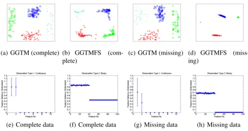
Visualisation results for GGTM and GGTMFS and saliency values estimated from the GGTMFS are presented in Figure 1 for both complete and incomplete data.
(a) GGTM (complete) (b) GGTMFS (com-plete)
(c) GGTM (missing) (d) GGTMFS (miss-ing)
(e) Complete data (f) Complete data (g) Missing data (h) Missing data
Fig. 1.GGTM and GGTMFS visualisations and saliencies of the synthetic mixed-type complete and missing datasets with10continuous and100binary features.10%of the continuous and binary complete data have been randomly removed to produce the missing data. GGTMFS visu-alisations quite often show more compact clusters compared to GGTM visuvisu-alisations. Saliencies plots show results as error bars from our cross-validation results. (e) and (g) show FS values of continuous features whereas (f) and (h) show FS values of binary features.
3.2 Real-world data: oil exploration
We applied the GGTMFS to two sets of oil exploration data from the Barents Sea: oil maturity and environmental parameters. The maturity data consists of17
continu-ous features with a large fraction (34%) of missing values and the environment data contains13continuous features with16% of missing values. Both datasets consist of
168samples. All the variables in the maturity dataset are important except feature 7, which has an environment influence that might make it behave differently, and feature
17, which is an environmental parameter. The features in the environment data are a combination of geochemical properties with variable importance. Features6,7,11and
12are more influenced by maturity than environment and hence their saliency values should be low.
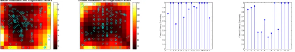
The resulting GGTMFS visualisation and saliency values plots are shown in Fig-ure 2. The GGTMFS plots are superimposed with magnification factor plots which en-able the user to observe the amount of stretching of the data-space manifold at different parts of the latent space [2]. This is useful to understand how the data is embedded in the data space, detect outliers and separate clusters. The magnification factors are rep-resented by colour shading in the projection manifold: the lighter the colour, the more stretch in the projection manifold. The GGTMFS visualisations on the oil data show
(a) Projection (matu-rity) (b) Projection (envi-ronment) (c) Saliencies (matu-rity) (d) Saliencies (envi-ronment)
Fig. 2. GGTMFS plot of the maturity (see (a)) and environment data (see (b)) and estimated feature saliency values of continuous features (see (c) and (d)).
that there is relatively little discrete structure (no clear clusters) in the data. The model was able to give a sensible saliency value(0.675)to the feature17in the maturity data as this variable is actually an environmental parameter. However, feature1should have a high saliency value according to the domain experts. In the environment data, the low saliency values of the features6and7make sense given that these features have a strong maturity influence. However, features11and12should also have low saliecny values, and feature10should have a high saliency value.
4
Conclusion
We derived a non-linear model for visualising a mixed-type dataset to simultaneously estimate saliency values both for complete and incomplete datasets. We called this model a generalised GTM with simultaneous feature saliency estimation (GGTMFS). Experimental visualisation results for both synthetic and real mixed-type datasets have shown that this model, unlike GGTM, provided more compact clusters especially in the presence of missing values and irrelevant features. More detailed results with other datasets are available in a technical report [12].
References
1. S. Alelyani, J. Tang, and H. Liu. Feature selection for clustering: A review. InData Cluster-ing: Algorithms and Applications, pages 29–60. Chapman and Hall/CRC, 2013.
2. C. Bishop, M. Svens´en, and C. K. I. Williams. Magnification factors for the GTM algorithm. InIn Proceedings IEE Fifth International Conference on Artificial Neural Networks, pages 64–69, 1997.
3. C. M. Bishop and M. Svensen. GTM: The generative topographic mapping.Neural Compu-atation, 10(1):215–234, 1998.
4. N. Bouguila. On multivariate binary data clustering and feature weighting. Comput. Stat. Data Anal., 54(1):120–134, 2010.
5. I. O. Caparroso. Variational Bayesian algorithms for generative topographic mapping and its extensions. PhD thesis, Universitat Polit`ecnica de Catalunya, 2008.
6. A. R. de Leon and K. C. Chough.Analysis of Mixed Data: Methods&Applications. Taylor
&Francis Group. Chapman and Hall/CRC, 2013.
7. A. Kab´an and M. Girolami. A combined latent class and trait model for the analysis and visu-alization of discrete data. IEEE Transactions on Pattern Analysis and Machine Intelligence, 23(8):859–872, 2001.
8. M. H. C. Law, M. A. T. Figueiredo, and A. K. Jain. Simultaneous feature selection and clustering using mixture models.IEEE Transactions on Pattern Analysis and Machine Intel-ligence, 26(9):1154–1166, 2004.
9. D. M. Maniyar and I. T. Nabney. Data visualization with simultaneous feature selection. In Computational Intelligence and Bioinformatics and Computational Biology, 2006. CIBCB ’06. 2006 IEEE Symposium on, pages 1–8, 2006.
10. S. Mumtaz.Visualisation of bioinformatics datasets. PhD thesis, Aston University, 2015. 11. S. Mumtaz, I. T. Nabney, and D. R. Flower. Novel visualization methods for protein data.
In IEEE Symposium on Computational Intelligence in Bioinformatics and Computational Biology (CIBCB), 2012, pages 198 –205, May 2012.
12. S. Mumtaz, M. F. Randrianandrasana, and I. T. Nabney. Mixed-type data visualisation and simultaneous feature saliency estimation using generalised generative topographic mapping. Technical report, Systems Analytics and Research Institute (SARI), Aston University, Birm-ingham, United Kingdom, 2015.
13. M. F. Randrianandrasana, S. Mumtaz, and I. T. Nabney. Visualisation of heterogeneous data with the generalised generative topographic mapping. InProceedings of the Tenth Inter-national Conference on Information Visualization Theory and Application, pages 233–238, 2015.
14. C. M. V. Silvestre, M. M. G. Cardoso, and M. A. T. Figueiredo. Clustering and selecting categorical features. InEPIA, volume 8154 ofLecture Notes in Computer Science, pages 331–342. Springer, 2013.
15. A. Vellido. Preliminary theoretical results on a feature relevance determination method for generative topographic mapping. Technical report, Universitat Politecnica de Catalunya (UPC)LSI-05-13-R, Barcelona, Spain, 2005.
16. A. Vellido. Assessment of an unsupervised feature selection method for generative topo-graphic mapping. InProceedings of the 16th International Conference on Artificial Neural Networks - Volume Part II, ICANN’06, pages 361–370, Berlin, Heidelberg, 2006. Springer-Verlag.
17. A. Vellido, P. J. G. Lisboa, and D. Vicente. Robust analysis of MRS brain tumour data using t-GTM.Neurocomputing, 69(7-9):754–768, 2006.
18. X. Wang and A. Kab´an. Finding uninformative features in binary data. InIntelligent Data Engineering and Automated Learning - IDEAL 2005, volume 3578 ofLecture Notes in Com-puter Science, pages 40–47. Springer Berlin Heidelberg, 2005.