University of California, Berkeley
U.C. Berkeley Division of Biostatistics Working Paper Series
Year Paper
A Causal Inference Approach for Constructing
Transcriptional Regulatory Networks
Biao Xing
∗Mark J. van der Laan
†∗Division of Biostatistics, School of Public Health, University of California, Berkeley, xing.biao@gene.com
†Division of Biostatistics, School of Public Health, University of California, Berkeley, laan@berkeley.edu
This working paper is hosted by The Berkeley Electronic Press (bepress) and may not be commer-cially reproduced without the permission of the copyright holder.
http://biostats.bepress.com/ucbbiostat/paper169 Copyright c2005 by the authors.
A Causal Inference Approach for Constructing
Transcriptional Regulatory Networks
Biao Xing and Mark J. van der Laan
Abstract
Transcriptional regulatory networks specify the interactions among regulatory genes and between regulatory genes and their target genes. Discovering transcriptional regulatory networks helps us to understand the underlying mechanism of complex cellular processes and responses. In this paper, we describe a causal inference ap-proach for constructing transcriptional regulatory networks using gene expression data, promoter sequences and information on transcription factor binding sites. The method rst identies active transcription factors under each individual exper-iment using a feature selection approach similar to Bussemaker et al. (2001), Keles et al. (2002) and Conlon et al. (2003). Transcription factors are viewed as ‘treatments’ and gene expression levels as ‘responses’. For every transcription factor and gene pair, a marginal structural model is built to estimate the causal eect of the transcription factor on the expression level of the gene. The model parameters can be estimated using either the G-estimation procedure or the IPTW estimator. The p-value associated with the causal parameter in each of these mod-els is used to measure how strongly a transcription factor regulates a gene. These results are further used to infer the overall regulatory network structures. We car-ried out simulations to assess the performance of our method in the estimation of a ctitious regulatory network. Our analysis of yeast data suggests that the method is capable of identifying signicant transcriptional regulatory interactions and the corresponding regulatory networks.
1
Introduction
Transcriptional regulatory networks specify the interactions among regula-tory genes and between regularegula-tory genes and their target genes. Discover-ing transcriptional regulatory networks is an important scientific task since it helps us to understand the underlying mechanism of complex cellular processes and responses.
There is a rich literature in methods for inferring regulatory networks. Lee et al. (2002) and Bar-Joseph et al. (2003) used the experiment-based genome-wide location analysis to investigate how yeast transcription factors (TF) bind to promoter sequences across genome, then constructed tran-scription factor-promoter binding networks to infer trantran-scriptional
regula-tory networks. Location analysis experiments provide in vivo evidence of
transcription factor binding to genes. However, physical binding does not di-rectly imply transcriptional regulatory activities. Moreover, location analy-sis experiments are often restricted to a certain growth condition. As a result, transcription factor-promoter binding network structures specific to other growth conditions may not be observed.
As microarray data on gene expression programs become available, var-ious statistical data mining tools have been devised for discovering (often more broadly defined) gene networks, for example, reverse engineering
ap-proaches (Somogyiet al., 1997; Lianget al., 1998; D’Haeseleeret al., 2000),
differential equations (Chenet al., 1999; D’Haeseleeret al., 1999), Bayesian
networks (Friedmanet al., 2000; Yooet al., 2002), etc. These methods often
require large number of time-course data or rely on very greedy computa-tional strategies.
Some other computational methods attempt to integrate gene expres-sion data, DNA sequences and functional annotations into a comprehensive
framework for discovering transcriptional regulatory networks (Pilpelet al.,
2001; Wanget al., 2002; Segalet al., 2003; Beer and Tavazoie, 2004). These
methods allow one to infer motif-to-gene or to some extent gene-to-gene regulatory networks.
Xing and van der Laan (2005) described a statistical approach for con-structing transcriptional regulatory networks using gene expression, pro-moter sequence and transcription factor binding site data. This approach first identifies transcription factors that are significantly associated with changes in gene expression profile under each experiment condition, then estimates the strength with which a regulatory gene regulates a potential
target gene, and finally averages evidence across experiments to infer the transcriptional regulatory network structures. This method employs a naive normal mixture model to estimate the strength with which a regulatory gene regulates a potential target gene. The normal mixture model is chosen for computational convenience. There are some concerns with the appropri-ateness of using a normal or other mixture models, e.g., the data may not appear to be normally distributed and consequently the model estimation may be poor. In addition, the mixture model is built on the transformed gene expression data for each transcription factor separately. There is not enough control for the possible confounding effects of other transcription factors on the estimated transcriptional regulatory interactions between the transcription factor under analysis and its potential target genes.
Here we describe an alternative approach based on causal inference methodology. We can view each gene as a subject and each transcription factor analogous to a ‘treatment’, which may have direct causal effects on the ‘responses’ (i.e., expression levels) of its target genes whose regulatory region is able to be bound by the transcription factor when it is active in an experiment. For genes whose regulatory region does not contain the tran-scription factor binding sites, there is no direct causal effect of the transcrip-tion factor on the expressions of those genes. More specifically, a ‘treatment’ variable is created for each transcription factor and coded into 1 when the transcription factor is active and 0 when the transcription factor is inactive in an experiment. Then for each experiment we will have a vector of ‘treat-ments’ associated with all the transcription factors, some of which may be active and some may be not. For different experiments, there will be dif-ferent combinations of ‘treatments’ as the active or inactive status of the transcription factors can be different across experiments. The changes in the expression level of a gene across experiments are seen as results from different combinations of ‘treatments’ under different experiment conditions. It should be noted that here a ‘treatment’ is not a usual treatment as we see in a controlled clinical trial, which is known prior to study and highly manipulable. In a typical microarray gene expression experiment, the tran-scription factor activities may not be deliberately controlled at all or may be under only limited manipulation. To our purpose of constructing tran-scriptional regulatory networks, we will need to first estimate the activities of transcription factors in a experiment and treat the transcription factor as ‘treatments’ that are causally responsible for the changes in gene expression levels.
Under this framework, we describe in the next section a causal inference approach for constructing transcriptional regulatory networks using gene expression data, promoter sequences and transcription factor binding sites. The method estimates ‘treatment’ code associated with each transcription factor under each experiment condition, then builds a marginal structural model for each gene and transcription factor pair to model the causal effect of the transcription factor on the expression level of the gene. Methods for estimating the model and inferring regulatory network structures are described. We conduct simulation studies to assess the performance of the proposed method in the estimation of a fictitious regulatory network. The results are summarized in Section 3. In Section 4, we apply the method to the yeast data to study the yeast transcriptional regulatory network. We conclude with a discussion of the uses and limitations of our method in Section 5.
2
Method
2.1 A brief introduction to causal inference methods
In causal inference, one concerns with estimation of acausal effect (a
para-meter with a causal interpretation) of a variable that can be manipulated (e.g., a treatment) on an outcome of interest, possibly adjusted for other
variables. Robins (1986, 1999a,b), Robins et al. (2000) and van der Laan
and Robins (2002) described causal inference methods for estimating the
average marginal causal effect of treatment A on outcome Y adjusted for
covariates V ⊂ W, based on longitudinal data involving time-independent
or time-dependent treatments. The marginal causal effects are defined using
the concept ofcounterfactual. The counterfactualYa represents the random
variable Y one would have observed, if, possibly contrary to the fact, one
would have ‘assigned’A =a, where a∈ A and A denotes a set of possible
treatments.
For a point treatment study, which is a special case of longitudinal study,
the observed data structure isO = (A, YA, W), whereW is a set of baseline
covariates. The full data structure is X = ((Ya:a∈ A), W), where Ya is
the counterfactual. A marginal structural model (MSM) can be used to
estimate the average marginal causal effect of A on Y (i.e., the effect of a
onE(Ya|V)) adjusted forV ⊂W as follows:
For example, we may specify a linear model likem(a, V|β) =β0+β1a+βvV,
whereβ0 is the intercept,β1 is the parameter for the marginal causal effect,
βv is a vector of regression coefficients, V is a subset of baseline covariates
to be adjusted. Let εa(β) = Ya −m(a, V|β). Then E(εa(β)|V) = 0 for
eacha∈ A. The estimation of causal parameterβ1 requires the assumption
of no unobserved confounders, i.e., g(A|X) = g(A|W), where g is a
prob-ability density (or mass) function, representing the treatment assignment
mechanism. In other words, this assumption states that treatmentAis
con-ditionally independent of the counterfactual outcomes given W, i.e., A is
randomized within each stratum ofW.
2.2 A causal inference method for constructing transcrip-tional regulatory networks
2.2.1 Data
Consider a particular organism such as the budding yeast. Let S(j, l) ∈
{A, C, T, G}denote the DNA base pair at the l-th position of the promoter
sequence of the j-th gene. Let S =¡S(j, l) : j = 1, . . . , J, l = 1, . . . , L(j)¢
denote all the promoter regions forJ genes, whereL(j) is the length of the
promoter sequence of thej-th gene. For simplicity, we can letL(j) =L for
allj = 1, . . . , J.
Let M = (M(1), . . . , M(K)) be a vector of DNA binding motifs,
possi-bly of variable lengths, which correspond to the binding sites of K known
transcription factors. Suppose we know the correspondence between a
tran-scription factorkand its producer gene g(k), fork= 1, . . . , K.
Consider now a particular gene expression experiment. Let Y = (Y(j) :
j = 1, . . . , J) be the observed gene expression vector. Given data of S,
M and Y, we can estimate the set of transcription factors that are
ac-tive under the experiment condition (where a transcription factor is ‘acac-tive’ refers to the situation in which the DNA binding site of the transcription factor is significantly associated with the changes in the genome-wide gene expression values), using linear regression with model selection or multiple
testing procedures as described in Bussemaker et al. (2001), Keles et al.
(2002), Conlon et al. (2003) and Xing and van der Laan (2005). These
procedures provide ways to transform single-experiment gene expression
data (Y), promoter sequences (S) and transcription factor binding sites
(M) into a vector of ‘treatment’ codes indicating which transcription
A = φ(Y, S, M) = (A(k) : k = 1, . . . , K) ∈ {0,1}K, where φ is a mapping
function corresponding to a procedure used to estimateA,A(k) = 1 means
the k-th transcription factor is active under the current experiment
condi-tion andA(k) = 0 otherwise. So, after having obtained this transformation,
we define our data as (A, Y, S, M).
Now suppose we have a collection ofngene expression experiments under
different conditions, possibly conducted for independent study purposes.
We assume that we can view these n gene expression experiments as n
i.i.d. draws from some population data generating distribution. Under this
assumption, we have n i.i.d. observations (Ai, Yi), i = 1, . . . , n and fixed
sequence dataS and M.
2.2.2 A causal inference model
We view the data analogous to data from a point treatment study, where the ‘treatment’ is whether a transcription factor is active or not. Consider a nonparametric marginal structural model which estimates the causal effect
of transcription factor k on gene expression j for each j = 1, . . . , J and
k= 1, . . . , K.
Let (j, k) be given. We now define a counterfactual gene expression
outcomeYa(j, k), which represents the expression level of genej one would
have observed if one had set/assigned A(k) = a, a ∈ {0,1}. Here Y0(j, k)
can be thought of as the expression of genej one would have observed if one
had knocked out geneg(k) (and thereby eliminating transcription factork),
or controlled transcription factorkto be inactive in the sense of binding and
regulation, whileY1(j, k) can be thought of as the expression value of gene
jone would have observed if one had controlled transcription factorkto be
actively involved in binding and regulation under the experiment condition.
Defineβ1(j, k) =EP[Y1(j, k)−Y0(j, k)]. Such a parameterβ1(j, k) measures
a marginal causal effect of A(k) on gene expression Y(j).
Let
G(k1, k2) =I(M(k1)⊂S(g(k2)),
that is, G(k1, k2) equals 1 if the binding site of transcription factor k1 is
contained in the promoter region of genek2, and it equals 0 otherwise. Let
G = (G(k1, k2) : k1 = 1, . . . , K, k2 = 1, . . . , K) denote the corresponding
K×K matrix. Note that matrix Grepresents a directed graph defined by
applying the rule “if G(k1, k2) = 1, then draw an arrow from k1 tok2” for
potential transcription factor connectivity matrix, denoted by
δ=¡δ(k1, k2) =I(There is a path from k1 tok2|G) : (k1, k2)∈ {1, . . . , K}2
¢
.
Let W(j, k) = ¡A(l) : l ∈ {1, . . . , K}, l 6= k and δ(k, l) = 0¢ be the
sub-vector of A corresponding to all transcription factors which are not
on the potential causal pathway from A(k) to Y(j), and are therefore
po-tential confounders of A(k). We now think of the full data as X(j, k) =
¡
Y0(j, k), Y1(j, k), W(j, k)
¢
. We link the observed data to this counterfac-tual data by the relation:
O(j, k) =¡Y(j) =YA(j, k), A(k), W(j, k)
¢
.
We assume there are no unmeasured confounders, in other words, A(k)
is conditionally independent of the counterfactual gene expressions¡Y0(j, k),
Y1(j, k)
¢
given W(j, k):
P(A(k) = 1|Y0(j, k), Y1(j, k), W(j, k)) =P(A(k) = 1|W(j, k)). If there would be variables affecting the absence/presence of transcription
factork(i.e.,A(k)), which are not included inW(j, k), then this assumption
could be violated. In addition, we assume the (j, k)-specific experimental
treatment assignment assumption holds, which states that 0 < P(A(k) =
1|W(j, k))<1 a.e. This now defines a nonparametric marginal structural
modelM(j, k) for the data structureO(j, k), and the parameter of interest
is given by β1(j, k).
We consider a simple (j, k)-specific nonparametric marginal structural
model as follows
E(Ya(j, k)) =β0(j, k) +I(M(k)⊂S(j))·β1(j, k)·a, (1)
wherea∈ {0,1}andβ1(j, k) is the causal parameter. The indicator function
I(M(k) ⊂ S(j)) constrains the model to estimate the causal parameter
only when there is a possible direct effect of transcription factork on gene
expression j.
We are interested in estimating the causal parameter β1(j, k) for every
gene and every transcription factor. Several strategies have been proposed for the estimation of the marginal causal parameters: (1) the G-computation estimation procedure (Robins, 1986, 1987), which requires the model for
EFX(Y|A, W) be correctly specified (whereFX represents the full data
dis-tribution); (2) the inverse probability of treatment weighted (IPTW)
and Robins, 2002), which requires the treatment mechanism (g(A|W)) be correctly specified; and (3) the double robust (DR) estimation procedure (Robins, 2000; van der Laan and Robins, 2002), which requires either the
model for EFX(Y|A, W) or the model for g(A|W) is correctly specified.
Since our analysis involves large scale genomic data, we may use the G-computation estimator or the IPTW estimator for G-computational ease.
2.2.3 The G-Computation estimation procedure
LetP andPn denote the true and empirical data distribution, respectively.
Since EP(Ya(j, k)) =E£E¡Y(j)|A(k) =a, W(j, k)¢¤, we can estimateE(Ya(j, k)) by EPn(Eb(Y(j)|A(k) =a, W(j, k)) = 1 n n X i=1 b E(Yi(j)|Ai(k) =a, Wi(j, k)).
Then the causal parameterβ1(j, k) =EP[Y1(j, k)−Y0(j, k)] is estimated by
ˆ
β1(j, k) =EPn h
b
E¡Y(j)|A(k) = 1, W(j, k)¢−Eb¡Y(j)|A(k) = 0, W(j, k)¢i.
The G-Computation estimation requires us to assume a suitable model
for E¡Y(j)|A(k) = a, W(j, k)¢. For simplicity, we may assume a linear
model of the form as follows:
E(Y(j)|A(k) =a, W(j, k)) =M(a, W(j, k)|γ) =γTZa,
where γ is the coefficients and Za = (1, a, W(j, k))T is a vector.
Sim-ilarly, we write Z1 = (1,1, W(j, k))T, Z0 = (1,0, W(j, k))T, and Z =
(1, A(k), W(j, k))T.
We first estimate the model based on the observed data, that is,
b
E(Y(j)|A(k), W(j, k)) =Mc(A(k), W(j, k)|γˆ) = ˆγTZ.
Then we estimateEb(Y(j)|A(k) = 1, W(j, k)) andEb(Y(j)|A(k) = 0, W(j, k))
using the above estimated model but usingZ1 and Z0 instead of Z.
To estimate V ar( ˆβ1(j, k)), i.e., the variance of the estimated causal
ef-fect, we need to estimate the influence curve of the estimator ˆβ1(j, k). We
describe the estimation procedure below. For notation convenience, we drop
Let M(a, W|γ) be the true data generating model, and Mc(a, W|ˆγ) be
the empirically estimated model. Then we can write β1 =EP[M(1, W)−
M(0, W)] and ˆβ1 =EPn[Mc(1, W)−Mc(0, W)]. Then ˆ β1−β1 ∼= EPn−P[M(1, W)− M(0, W)] +EP[( ˆM − M)(1, W)−( ˆM − M)(0, W)] = 1 n n X i=1 [M(1, W)− M(0, W)]−E[M(1, W)− M(0, W)] +[1 n n X i=1 (Ziεi(γ))T][E(ZZT)]−1E(Z1−Z0), whereε(γ) =Y −ˆγTZ. ˆ
β1 is a consistent estimator for β1. Under regularity condition, ˆβ1−β1
is asymptotically linear with influence curve being
IC(O) = (M(1, W)− M(0, W))−E(M(1, W)− M(0, W))
+(Zε(γ))T[E(ZZT)]−1E(Z1−Z0).
So, √
n( ˆβ1−β1)→ N(0, σ2 =V ar(IC)).
Note IC(Oi) can be estimated by
c IC(Oi) = (Mc(1, Wi)−Mc(0, Wi))−n1 n X i=1 (Mc(1, Wi)−Mc(0, Wi)) +(Ziεi(γ))T " 1 n n X i=1 (ZiZiT) #−1" 1 n n X i=1 (Z1i−Z0i) # ,
and σ2 can be estimated by
ˆ σ2 =V ard(IC) = 1 n n X i=1 Ã c ICi− 1n n X i=1 c ICi !2 .
The Wald test statistic forH0:β1= 0 is
T =
√
nβˆ1 ˆ
2.2.4 The IPTW estimation procedure
The IPTW estimator is constructed by the following estimating function:
Dh(O|β, g) = h(A, V)ε(β)
g(A|W) , (2)
wherehis a vector function ofAandV, andgis a conditional distribution of
AgivenW (i.e., treatment mechanism). It is shown that, under the
assump-tion of no unobserved confounders (NUC) and the experimental treatment assignment (ETA) assumption, the above estimating function is unbiased
forβ, i.e., E(Dh(O|β, g)) = 0 (Neugebauer and van der Laan, 2002).
As suggested by Robins (1999b), a sensible choice of h is h(A, V) =
g(A|V) ∂
∂βm(A, V|β). Consequently, the estimate of β can be obtained by
regressing Y over A with weights wt = gg((AA||WV)). For example, if we
spec-ify a marginal structural model as (1), we may simply choose h(A) =
g(A)∂β∂ m(A|β). We then estimate β using weighted least square
estima-tion by regressingY overA with weights wt= g(gA(A|W)).
To estimate the weight, we need to model the treatment mechanism
g(A|W). For our particular problem, A is binary with A = 1 if the
tran-scription factor under study is active and A = 0 otherwise. A convenient
choice of the model forg(A|W) is the logistic regression model, for example,
logit¡g(A(k) = 1|W(j, k) =w(j, k))¢=γ0+
X
(m:A(m)∈W(j,k))
γmA(m). (3)
So, the estimated weight is wti = ˆg(Ai(k)=1)
ˆ
g(Ai(k)=1|Wi(k)=wi(k)) for i = 1, . . . , n,
where ˆg(Ai(k) = 1|Wi(k) = wi(k)) is estimated using Equation (3) and
ˆ
g(Ai(k) = 1) = 1
n
Pn
i I(Ai(k) = 1).
2.2.5 Inference on the regulatory network structures
After fitting the causal marginal structural model (1) for every gene and
every transcription factor, we can obtain aJ byKp-value matrix,P, whose
element is defined by
Pjk =
½
p-value w.r.t the test of H0:β1(j, k) = 0 ifM(k)⊂S(j),
The J by K transcriptional regulatory interaction matrix (B) can be estimated by
ˆ
Bjk =I(Pjk ≤p) forj= 1, . . . , J and k= 1, . . . , K, (5)
wherep is a user specified p-value threshold (e.g.,p= 0.001).
Note ˆBjk = 1 may be interpreted as that the marginal causal effect
of the k-th transcription factor on the j-th gene is significantly different
from zero. Therefore, we infer that there is a transcriptional regulatory
interaction between thek-th transcription factor and the j-th gene.
We then can use the methods described in Lee et al. (2002) and Xing
and van der Laan (2005) to identify network motifs and assemble the overall regulatory network.
3
Simulation Studies
We conduct simulations to show how the proposed computational approach performs in re-constructing the underlying regulatory network structure. The parameter of interest is the transcriptional regulatory interaction
ma-trix B, which may be regarded as a 2-dimensional representation of the
underlying network. Note that B is constructed in simulation studies but
not known in practice.
3.1 Constructing a fictitious regulatory network
We consider a fictitious transcriptional regulatory network consisting of 10 transcription factors and 90 genes. For simplicity, suppose that five of the transcription factors are inducers and the remaining five are repressors. Also suppose that one-third of the genes are regulated by at least one inducer but no repressors, another one-third regulated by at least one repressor but no inducers, and the remaining one-third regulated by none of the 10 tran-scription factors. We randomly construct a binary-valued trantran-scriptional
regulatory interaction matrixB, which satisfies the above condition.
3.2 Constructing a fictitious motif abundance matrix
Next we construct a fictitious motif abundance matrixX, which indicates
factors in the promoter sequences of each gene. Note thatX is available in
practice based on sequence data M and S. A necessary condition for the
k-th transcription factor transcriptionally regulates thej-th gene is that the
j-th gene must have at least one binding site for thek-th transcription factor
in its promoter region. In other words,Bjk = 1 implies that Xjk = 1. It is
also true that Xjt = 0 implies that Bjk = 0. However, when Xjk = 1, Bjk
may be 1 or 0. We regard the situation thatBjk = 0 and Xjk = 1 (i.e. a
transcription factor does not regulate a gene even though the gene promoter is abundant with binding sites of the transcription factor) as systematic noise in the motif abundance matrix.
We use the following rules to construct the motif abundance matrixX:
• IfBjk = 1, then Xjk = 1;
• IfBjk = 0, then Xjk ∼Bernoulli {0,1}withP(Xjk = 1) =δ.
We consider three values forδ, i.e.,δ= 0.10,0.20,0.30, representing different
levels of systematic error in the motif abundance matrixX.
3.3 Simulating gene expression data for different conditions
Next we generate data that resemble the situation that we have a collection
ofnexperiments. Each experiment is seen as a realization of certain part of
the true underlying regulatory network.
To do so, for each i = 1, . . . , n, we draw a random subset τ(i) ⊆
{1, . . . , K}, with a random size|τ(i)| ∼Uniform {3, . . . ,7}.
The fictitious gene expression data are generated using a multiple linear model as follows
Yji =β0+
X
k∈τ(i)
βtXjk+²ji,
wherejindexes genes,iindexes experiments,kindexes transcription factors,
β’s are coefficients,²j is the gene-specific random error,E(²j) = 0, andτ(i)
is the set of transcription factors that are active under thei-th experiment.
For simplicity, we assumeβ0 = 0,β~t= (0.25, 0.30, 0.35, 0.40, 0.45, -0.25,
-0.30, -0.35, -0.40, -045), and ²j =² ∼N(0, σ2). We consider three values
forσ, i.e., σ= 0.25,0.50,0.75, representing different levels of random errors
We estimate ˆB based on the generated data and compute the overall error rate and false positive rate as defined in Section 3.4. We repeat the procedures 100 times and get average estimates of the error rates.
3.4 Error in estimation
To assess the error in estimation, we define the overall error rate (OER), the false positive rate (FPR) and the false negative rate (FNR) as follows to indicate the overall accuracy, node accuracy and node completeness re-spectively: OER= 1 J×K X j,k I(Bjk 6= ˆBjk), F P R=X j,k I((Bjk = 0) and ( ˆBjk = 1))/X j,k I( ˆBjk = 1), F N R=X j,k I((Bjk = 1) and ( ˆBjk = 0))/ X j,k I( ˆBjk = 0). 3.5 Simulation results
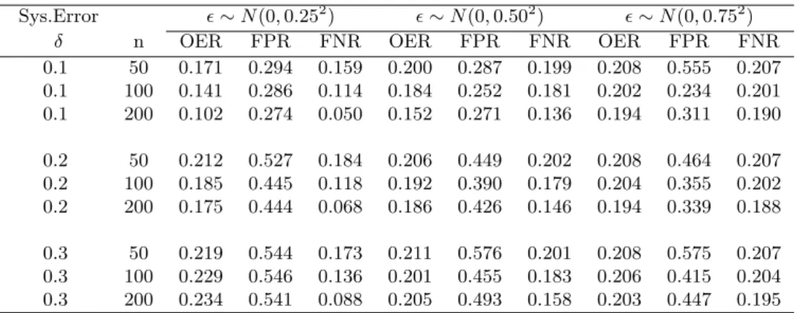
The simulation results (using the IPTW estimation) are shown in Table
1, where ² ∼ N(0, σ2) with σ = 0.25,0.5,0.75 indicates increasing level of
random error in gene expression measurements, and δ = 0.1,0.2,0.3
indi-cates increasing level of systematic error in the constructed motif abundance
matrixX. Three sample sizes (n=50, 100, 200) are used.
We see that the all the OER, FPR and FNR increase as the systematic error increases and decrease as the sample size increases. The OER and FNR also increase as the random error increases. The FPR may also increase as the random error increases but the trend is not consistent. When the sys-tematic error and random error are small and the sample size is moderately large, the overall error rate, the false positive rate and the false negative rate are reasonably small. In real world, we do not know the magnitude of the systematic error with respect to the relationship between motif abundance and transcriptional regulatory interaction. If the systematic error is very large, we would not expect some of the motif detection methods
(Busse-maker et al., 2001; Keles et al., 2002; Conlon et al., 2003) to work well.
Successful results from these studies imply that the assumption of a small or moderate systematic error may be realistic in real data analysis.
[Table 1 about here.]
4
Data Analysis
We apply our method to study the transcriptional regulatory network inS.
Cerevisiae (budding yeast) based on analysis of a large collection of DNA microarray experiments.
4.1 Data
4.1.1 DNA microarray experiments
We collect 658 DNA microarray experiments on yeast gene expression
pro-grams under various conditions: 7 on diauxic shift (DeRisiet al., 1997), 10
on sporulation (Chu et al., 1998), 60 on cell cycle (Spellman et al., 1998),
4 on adaptive evolution (Ferea et al., 1999), 173 on environmental stress
(Gasch et al., 2000), 6 on Copper regulation (Gross et al., 2000), 300 on
diverse mutations and chemical treatments (Hugheset al., 2000), 8 on Pho
metabolism (Ogawa et al., 2000), 12 on SNF/SWI mutants (Sudarsanam
et al., 2000), 26 on FKH1 and FKH2 roles during cell cycle (Zhu et al.,
2000), and 52 on DNA damage (Gaschet al., 2001).
Prior to analysis, the data are normalized by subtracting the
genome-wise median for every experiment. In addition, the log2(ratios) are truncated
by±log2(20).
4.1.2 Promoter sequences
We extract promoter sequences of 700 bps in length in the upstream non-coding region [-700, -1] for 6136 ORFs using the SCPD database (Zhu and Zhang, 1999).
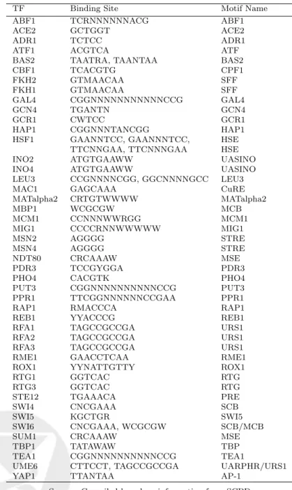
4.1.3 Transcription factor binding sites
We collect known binding sites for 46 yeast transcription factors from SCPD
(Zhu and Zhang, 1999), TRANSFAC (Wingenderet al., 1996), and YPD of
[Table 2 about here.]
4.2 Analysis results
4.2.1 Estimated transcriptional regulatory interactions
The estimated number of transcriptional regulatory interactions between transcription factors and genes is a function of cut-off value used. Table 3 shows the results at different cut-off levels.
[Table 3 about here.]
In our analysis, we choose p = 0.001 as a threshold to infer the yeast
transcriptional regulatory interaction. The estimated transcriptional regu-latory interaction matrix is then used to find network motifs and network structures.
4.2.2 Network motifs
Network motifs are the simplest units of the network architecture, which
suggest models for regulatory mechanism that can be tested. Lee et al.
(2002) described six regulatory network motifs in terms of transcription factor binding (see Figure 1) and algorithms to find them. We redefine the network motifs in terms of transcriptional regulatory interaction as fol-lows: (a) Auto-regulation motif, in which a regulator gene regulates its own expression; (b) Feed-forward loop motif, in which a master regulator reg-ulates the second regulator and both regulate a common target gene; (c) Multi-component loop motif, in which regulator(1) regulates regulator(2), ..., regulator(n-1) regulates regulator(n), and regulator(n) regulates
regu-lator(1), where n ≥ 2; (d) Single input motif, in which a single regulator
uniquely regulates a set of target genes; (e) Multi-input motif, in which a set of regulators regulate a set of target genes together; and (f) Regulator chain motif, in which regulator(1) regulates regulator(2), ..., regulator(n-1)
regulates regulator(n), wheren≥2 and the chain ends if regulator(n) does
not directly regulate any other regulator that is not on the chain. [Figure 1 about here.]
We used the algorithms described in Lee et al. (2002) and Xing and van der Laan (2005) to find interesting transcriptional regulatory network motifs. We found 6 auto-regulated genes, 37 feed-forward loops, 1 multi-component loops, 26 single-input modules, 254 multi-input modules and 96 regulator chains, based on the estimated transcriptional regulatory interac-tions matrix for 46 transcription factors and 6136 genes, at a threshold of
p= 0.001.
To assess the significance of the findings, we compared our results with
those from Leeet al. (2002). Our analysis involves 46 transcription factors,
the analysis of Lee et al. (2002) involves 106 transcription factors. We
have 33 transcription factors in common. However, since the presence of additional transcription factors affects the finding of almost all the network motifs, particularly the single-input and multi-input modules and regulator chains (a result of the network motif finding algorithm). So the comparison focuses on only auto-regulation motif and feed-forward loop motif.
[Table 4 about here.]
Table 4 lists genes that are likely to be autoregulated. At the threshold of
p= 0.001, we found 6 regulator genes (out of 46) that may be autoregulated:
ADR1, MIG1, NDT80, RAP1, ROX1 and TBP1. Among these, RAP1 was
also identified as an autoregulated gene in Lee et al. (2002), and NDT80
and ROX1 were computationally identified as autoregulated genes in Xing and van der Laan (2005).
NDT80p functions at pachytene of yeast gametogenesis (sporulation) to activate transcription of a set of genes required for both meiotic division and gamete formation. There is evidence that NDT80p activates its own tran-scription through an upstream MSE consensus site (Chu and Herskowitz,
1998; Lindgrenet al., 2000).
The ROX1 gene encodes a heme-induced repressor of hypoxic genes in yeast. Experiments indicated that ROX1p is capable of binding to its own
upstream region and represses its own expression (Deckert et al., 1995).
ROX1 was included in Lee et al. (2002), but was not identified as
auto-regulated.
At a less restrictive threshold level, STE12 and SWI4 are also found to be autoregulated, which were also identified as autoregulated genes in Lee
et al.(2002) and Xing and van der Laan (2005). However, we did not found literature support for ADR1, MIG1 and TBP1. Regulation mechanisms for
these genes are not completely clear.
We found 37 feed-forward loops involving 23 transcription factors at the
threshold level of p = 0.001. Among these, RAP1-HSF1 was also
identi-fied in Lee et al. (2002). ADR1, LEU3, MIG1 and TBP1 seem to form a
feed-forward loop with MSN4, as the same relationships were also found computationally in Xing and van der Laan (2005).
4.2.3 Overall transcriptional regulatory network
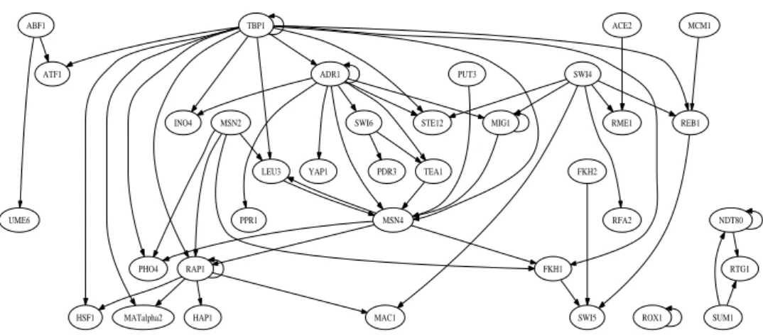
We can construct the overall transcriptional regulatory network based on the estimated transcriptional regulatory interaction matrix. Figure 2 shows the estimated regulator network, which consists of 36 regulatory genes that have estimated transcriptional regulatory interactions with either themselves (i.e., autoregulation) or other regulators. The remaining 10 regulatory genes that are involved in the analysis but have no estimated transcriptional regulatory interactions with any regulators are not shown. Each of the 46 regulatory genes involved in the analysis has its own set of potential target genes, which are not shown in the graph neither to make it clear.
[Figure 2 about here.]
The analysis results show that the proposed statistical approach is ca-pable of identifying significant transcriptional regulatory interactions and the corresponding regulatory network structures. For example, the con-structed network directly connects most of the regulators that are known to regulate the yeast cell cycle process, such as RME1, SWI4, SWI5, ACE2, MCM1, FKH1 and FKH2, to form a sub-network for cell cycle regulation. Among the estimated cell cycle related transcriptional regulatory interac-tions, some have already been experimentally confirmed. For example,
ACE2 induces the meiosis repressor RME1 (Toone et al., 1995; McBride
et al., 1999); REB1 directly increases the mRNA abundance of SWI5 (Svet-lov and Cooper, 1995); FKH2 upregulates cell-cycle dependent expression
of the CLB2 cluster of genes, which include SWI5 and ACE2 (Boroset al.,
2003).
The method is capable of revealing the transcriptional regulatory net-work structure that is not obvious under a single experiment condition. For example, our analysis suggests that SUM1 transcriptionally regulates NDT80, and NDT80 is auto-regulated. In fact, SUM1p and NDT80p bind
competitively to the MSE sites in the promoter region of NDT80 and result in very different consequences: NDT80p activates the expression of NDT80, but SUM1p represses the expression of NDT80 (Pak and Segall, 2002). The cross link between SUM1 and NDT80 may not be observed in a location analysis based on only one kind of growth condition.
5
Discussion
In this paper we described a causal inference model based approach for constructing transcriptional regulatory networks using data on gene expres-sion, promoter sequence, and transcription factor binding sites. The method views an active transcription factor under a given experiment analogous to a point treatment and the gene expressions as responses. The concept of coun-terfactual gene expression is introduced and a marginal structural model is built for every gene and transcription factor pair to infer the regulatory in-teractions. Our simulation studies show that the overall error rate, false positive and false negative error rates in the estimated transcriptional regu-latory networks are expected to be small or moderate if the systematic noise and the random error in the data is small and the sample size is moderately large. Our analysis based on 658 microarray experiments on yeast gene ex-pression programs and 46 transcription factors suggests that the method is capable of identifying significant transcriptional regulatory interactions and uncovering the corresponding network structures.
The computational approach is based on available gene expression and sequence data, so it is time-wise and resource-wise more efficient than the experiment-based methods (e.g., location analysis). It is especially suit-able for mining the fast accumulating microarray data on gene expressions under various experiment conditions. Since data from many different experi-ment conditions are explored, our method is particularly advantageous over location analysis and single transcription factor perturbation experiment based approaches for its capability of finding the transcriptional regulatory network structure that is not fully observable under a single experiment condition, for example, the interaction between SUM1 and NDT80.
As compared with our previous method (Xing and van der Laan, 2005), this method is time-wise more efficient since it does not use the naive normal mixture model and the IPTW estimation of the marginal structural models is faster than the EM algorithm based estimation of the mixture models. But the MSM needs the no unmeasured confounders (NUC) assumption and the
experimental treatment assignment (ETA) assumption to obtain consistent estimate of the causal effects. We usually are not able to check whether these assumptions all hold without further knowledge except for the data. The analysis based on data from real experiments seems to suggest that the two methods can be complementary to each other in maximizing significant findings.
The method has some the limitations. First, it may fail to estimate the regulatory interactions of a transcription factor that results in only subtle change in the genome-wide gene expression profile. Second, the method relies on knowledge of transcription factor binding sites. The number of transcription factors with known consensus binding sites is small and their functional coverage is somewhat limited. However, this may not be a prob-lem when more and more transcription factor binding sites are characterized and added to our knowledge. Also, we may use putative transcription fac-tor binding sites in the analysis. Using putative transcription facfac-tor binding sites will increase the error rates in estimation, but the constructed networks should suggest more models for further testing.
References
Bar-Joseph, Z., Gerber, G. K., Lee, T. I., Rinaldi, N. J., Yoo, J. Y., Robert, F., Gordon, D. B., Fraenkel, E., Jaakkola, T. S., Young, R. A. and Gifford, D. K. (2003) Computational discovery of gene modules and regulatory
networks. Nature Biotechnology,21(11), 1337–42.
Beer, M. A. and Tavazoie, S. (2004) Predicting gene expression from
se-quence. Cell,117, 185–198.
Boros, J., Lim, F. L., Darieva, Z., Pic-Taylor, A., Harman, R., Morgan, B. A. and Sharrocks, A. D. (2003) Molecular determinants of the
cell-cycle regulated mcm1p-fkh2p transcription factor complex. Nucleic Acids
Res,31, 2279–83.
Bussemaker, H. J., Li, H. and Siggia, E. D. (2001) Regulatory element
detection using correlation with expression. Nature Genetics, 27, 167–
171.
Chen, T., He, H. L. and Church, G. M. (1999) Modeling gene expression
Chu, S., DeRisi, J., Eisen, M. B., Mulholland, J., Botstein, D., Brown, P. O. and Herskowitz, I. (1998) The transcriptional program of sporulation in
budding yeast. Science,282, 699–705.
Chu, S. and Herskowitz, I. (1998) Gametogenesis in yeast is regulated by a
transcriptional cascade dependent on ndt80. Mol Cell,1, 685–696.
Conlon, E. M., Liu, X. S., Lieb, J. D. and Liu, J. S. (2003) Integrating
sequence motif discovery and microarray analysis. Proc. Nat’l Acad. Sci.,
100, 3339–44.
Deckert, J., Perini, R., Balasubramanian, B. and Zitomer, R. S. (1995) Mul-tiple elements and auto-repression regulate rox1, a repressor of hypoxic
genes in saccharomyces cerevisiae. Genetics,139, 1149–58.
DeRisi, J. L., Iyer, V. R. and Brown, P. O. (1997) Exploring the metabolic
and genetic control of gene expression on a genomic scale. Science,278,
680–686.
D’Haeseleer, P., Liang, S. and Somogyi, R. (2000) Genetic network inference:
From co-expression clustering to reverse engineering. Bioinformatics,16,
707–726.
D’Haeseleer, P., Wen, X., Fuhrman, S. and Somogyi, R. (1999) Linear
mod-eling of mrna expression levels during cns development and injury. Proc.
Pac. Symp. Biocomputing,4, 41–52.
Ferea, T. L., Botstein, D., Brown, P. O. and Rosenzweig, R. F. (1999) Sys-tematic changes in gene expression patterns following adaptive evolution
in yeast. Proc Natl Acad Sci,96(17), 9721–6.
Friedman, N., Linial, M., Nachman, I. and Pe’er, D. (2000) Using bayesian
networks to analyze expression data. J. Comput. Biol.,7, 601–620.
Gasch, A. P., Huang, M., Metzner, S., Botstein, D., Elledge, S. J. and Brown, P. O. (2001) Genomic expression responses to dna-damaging agents and
the regulatory role of the yeast atr homolog mec1p. Mol Biol Cell, 12,
2987–3003.
Gasch, A. P., Spellman, P. T., Kao, C. M., Carmel-Harel, O., Eisen, M. B., Storz, G., Botstein, D. and Brown, P. O. (2000) Genomic expression
pro-grams in the response of yeast cells to environmental changes. Mol Biol
Gross, C., Kelleher, M., Iyer, V. R., Brown, P. O. and Winge, D. R. (2000) Identification of the copper regulon in saccharomyces cerevisiae by dna
microarrays. J Biol Chem,275, 32310–6.
Hodges, P. E., McKee, A. H. Z., Davis, B. P., Payne, W. E. and Garrels, J. I. (1999) Yeast proteome database (ypd): a model for the organization
and presentation of genome-wide functional data. Nucleic Acids Res.,27,
69–73.
Hughes, T. R., Marton, M. J., Jones, A. R., Roberts, C. J., Stoughton, R., Armour, C. D., Bennett, H. A., Coffey, E., Dai, H., He, Y. D., Kidd, M. J., King, A. M., Meyer, M. R., Slade, D., Lum, P. Y., Stepaniants, S. B., Shoemaker, D. D., Gachotte, D., Chakraburtty, K., Simon, J., Bard, M. and Friend, S. H. (2000) Functional discovery via a compendium of
expression profiles. Cell,102, 109–126.
Keles, S., van der Laan, M. J. and Eisen, M. B. (2002) Identification of
regulatory elements using a feature selection method. Bioinformatics,18,
1167–1175.
Lee, T. I., Rinaldi, N. J., Robert, F., Odom, D. T., Bar-Joseph, Z., Gerber, G. K., Hannett, N. M., Harbison, C. R., Thompson, C. M., Simon, I., Zeitlinger, J., Jennings, E. G., Murray, H. L., Gordon, D. B., Ren, B., Wyrick, J. J., Tagne, J., Volkert, T. L., Fraenkel, E., Gifford, D. K. and Young, R. A. (2002) Transcriptional regulatory networks in saccharomyces
cerevisiae. Science,298, 799–804.
Liang, S., Fuhrman, S. and Somogyi, R. (1998) Reveal: A general reverse
engineering algorithm for inference of genetic network architectures.Proc.
Pac. Symp. Biocomput.,3, 18–29.
Lindgren, A., Bungard, D., Pierce, M., Xie, J., Vershon, A. and Winter, E. (2000) The pachytene checkpoint in saccharomyces cerevisiae requires the
sum1 transcriptional repressor. Embo Journal,19, 6489–6497.
McBride, H. J., Yu, Y. and Stillman, D. J. (1999) Distinct regions of the swi5
and ace2 transcription factors are required for specific gene activation. J
Biol Chem,274, 21029–21036.
Neugebauer, R. and van der Laan, M. J. (2002) Why prefer double robust
estimates? illustration with causal point treatment studies.U.C. Berkeley
Ogawa, N., DeRisi, J. and Brown, P. O. (2000) New components of a sys-tem for phosphate accumulation and polyphosphate metabolism in
sac-charomyces cerevisiae revealed by genomic expression analysis. Mol Biol
Cell, 11, 4309–4321.
Pak, J. and Segall, J. (2002) Regulation of the premiddle and middle phases of expression of the ndt80 gene during sporulation of saccharomyces
cere-visiae. Mol Cell Biol,22, 6417–29.
Pilpel, Y., Sudarsanam, P. and Church, G. (2001) Identifying regulatory
networks by combinatorial analysis of promoter elements. Nat. Genet.,
29, 153–159.
Robins, J. M. (1986) A new approach to causal inference in mortality studies with sustained exposure periods - application to control of the healthy
worker survivor effect. Mathematical Modelling,7, 1393–1512.
Robins, J. M. (1987) A graphical approach to the identification and esti-mation of causal parameters in mortality studies with sustained exposure
periods. Journal of Chronic Disease,40, 139s–161s.
Robins, J. M. (1999a) Association, causation, and marginal structural mod-els. Synthese,121, 151–179.
Robins, J. M. (1999b) Marginal structural models versus structural nested models as tools for causal inference. In Halloran, M. and Berry, D. (eds.),
Statistical Models in Epidemiology: The Environment and Clinical Trials, pp. 95–134. Springer-Verlag, NY.
Robins, J. M. (2000) Robust estimation in sequentially ignorable missing
data and causal inference models. InProceedings of the American
Statis-tical Association 1999, pp. 6–10.
Robins, J. M., Hernan, M. A. and Brumback, B. (2000) Marginal structural
models and causal inference in epidemiology. Epidemiology,11, 550–560.
Segal, E., Yelensky, R. and Koller, D. (2003) Genome-wide discovery of
transcriptional modules from dna sequence and gene expression.
Bioin-formatics,19, i273–i282.
Somogyi, R., Fuhrman, S., Askenazi, M. and Wuensche, A. (1997) The gene expression matrix: Towards the extraction of genetic network
architec-tures. Proc. of Second World Congress of Nonlinear Analysts, 30(3),
Spellman, P. T., Sherlock, G., Zhang, M. Q., Iyer, V. R., Anders, K., Eisen, M. B., Brown, P. O., Botstein, D. and Futcher, B. (1998) Comprehen-sive identification of cell cycle-regulated genes of the yeast saccharomyces
cerevisiae by microarray hybridization. Mol Biol Cell,9, 3273–97.
Sudarsanam, P., Iyer, V. R., Brown, P. O. and Winston, F. (2000) Whole-genome expression analysis of snf/swi mutants of saccharomyces
cere-visiae. Proc Natl Acad Sci,97, 3364–9.
Svetlov, V. V. and Cooper, T. G. (1995) Review: compilation and char-acteristics of dedicated transcription factors in saccharomyces cerevisiae.
Yeast,11, 1439–84.
Toone, W. M., Johnson, A. L., Banks, G. R., Toyn, J. H., Stuart, D., Wittenberg, C. and Johnston, L. H. (1995) Rme1, a negative regulator
of meiosis, is also a positive activator of g1 cyclin gene expression. Embo
Journal,14, 5824–32.
van der Laan, M. J. and Robins, J. (2002) Unified methods for Censored
Longitudinal Data and Causality. Springer-Verlag, New York.
Wang, W., Cherry, J. M., Botstein, D. and Li, H. (2002) A systematic approach to reconstructing transcription networks in saccharomyces
cere-visiae. Proc. Natl. Acad. Sci.,99, 16893–98.
Wingender, E., Dietze, P., Karas, H. and Knppel, R. (1996) Transfac: A
database on transcription factors and their dna binding sites. Nucleic
Acids Res.,24, 238–241.
Xing, B. and van der Laan, M. J. (2005) A statistical method for con-structing transcriptional regulatory networks using gene expression and
sequence data. Journal of Computational Biology,12, 229–246.
Yoo, C., Thorsson, V. and Cooper, G. F. (2002) Discovery of causal rela-tionships in a gene-regulation pathway from a mixture of experimental
and observational dna microarray data. Proc. Pac. Symp. Biocomput.,7,
498–509.
Zhu, G., Spellman, P. T., Volpe, T., Brown, P. O., Botstein, D., Davis, T. N. and Futcher, B. (2000) Two yeast forkhead genes regulate the cell cycle
and pseudohyphal growth. Nature,406, 90–94.
Zhu, J. and Zhang, M. Q. (1999) Scpd: A promoter database of yeast
Figure 1: Transcriptional regulatory network motifs: (a) Auto-regulation, (b) Feed-forward loop, (c) Multi-component loop, (d) Single-input motif, (e) Multi-input motif, and (f) Regulator chain motif. Transcription factors are indicated by blue circles and genes by green boxes. Solid arrows indicate regulatory interaction between transcription factors and their target genes. Dashed arrows link transcription factors and their producer genes. The
ABF1 ATF1 UME6 ROX1 SUM1 NDT80 RTG1 ACE2 RME1 ADR1 INO4 MIG1 MSN4 PPR1 STE12 SWI6 TEA1 YAP1 FKH1 LEU3 PHO4 RAP1 PDR3 FKH2 SWI5 MCM1 REB1 MSN2 HAP1 HSF1 MATalpha2 MAC1 PUT3 SWI4 RFA2 TBP1
Figure 2: Estimated yeast transcriptional regulatory network. Ovals indi-cate regulatory genes. Arrows indiindi-cate the direction of transcriptional reg-ulatory interactions. Regulators without significant interactions with other regulators are not shown. The potential target genes of each regulator are not shown.
Table 1: Average error rates in the estimated transcriptional regulatory interaction matrices
Sys.Error ²∼N(0,0.252) ²∼N(0,0.502) ²∼N(0,0.752)
δ n OER FPR FNR OER FPR FNR OER FPR FNR
0.1 50 0.171 0.294 0.159 0.200 0.287 0.199 0.208 0.555 0.207 0.1 100 0.141 0.286 0.114 0.184 0.252 0.181 0.202 0.234 0.201 0.1 200 0.102 0.274 0.050 0.152 0.271 0.136 0.194 0.311 0.190 0.2 50 0.212 0.527 0.184 0.206 0.449 0.202 0.208 0.464 0.207 0.2 100 0.185 0.445 0.118 0.192 0.390 0.179 0.204 0.355 0.202 0.2 200 0.175 0.444 0.068 0.186 0.426 0.146 0.194 0.339 0.188 0.3 50 0.219 0.544 0.173 0.211 0.576 0.201 0.208 0.575 0.207 0.3 100 0.229 0.546 0.136 0.201 0.455 0.183 0.206 0.415 0.204 0.3 200 0.234 0.541 0.088 0.205 0.493 0.158 0.203 0.447 0.195
Table 2: Some yeast transcription factors and their specific binding sites
TF Binding Site Motif Name
ABF1 TCRNNNNNNACG ABF1
ACE2 GCTGGT ACE2
ADR1 TCTCC ADR1
ATF1 ACGTCA ATF
BAS2 TAATRA, TAANTAA BAS2
CBF1 TCACGTG CPF1 FKH2 GTMAACAA SFF FKH1 GTMAACAA SFF GAL4 CGGNNNNNNNNNNNCCG GAL4 GCN4 TGANTN GCN4 GCR1 CWTCC GCR1
HAP1 CGGNNNTANCGG HAP1
HSF1 GAANNTCC, GAANNNTCC, HSE
TTCNNGAA, TTCNNNGAA HSE
INO2 ATGTGAAWW UASINO
INO4 ATGTGAAWW UASINO
LEU3 CCGNNNNCGG, GGCNNNNGCC LEU3
MAC1 GAGCAAA CuRE
MATalpha2 CRTGTWWWW MATalpha2 MBP1 WCGCGW MCB MCM1 CCNNNWWRGG MCM1 MIG1 CCCCRNNWWWWW MIG1 MSN2 AGGGG STRE MSN4 AGGGG STRE NDT80 CRCAAAW MSE PDR3 TCCGYGGA PDR3
PHO4 CACGTK PHO4
PUT3 CGGNNNNNNNNNNCCG PUT3
PPR1 TTCGGNNNNNNCCGAA PPR1
RAP1 RMACCCA RAP1
REB1 YYACCCG REB1
RFA1 TAGCCGCCGA URS1
RFA2 TAGCCGCCGA URS1
RFA3 TAGCCGCCGA URS1
RME1 GAACCTCAA RME1
ROX1 YYNATTGTTY ROX1
RTG1 GGTCAC RTG
RTG3 GGTCAC RTG
STE12 TGAAACA PRE
SWI4 CNCGAAA SCB
SWI5 KGCTGR SWI5
SWI6 CNCGAAA, WCGCGW SCB/MCB
SUM1 CRCAAAW MSE
TBP1 TATAWAW TBP
TEA1 CGGNNNNNNNNNNCCG TEA1
UME6 CTTCCT, TAGCCGCCGA UARPHR/URS1
YAP1 TTANTAA AP-1
Source: Compiled based on information from SCPD, TRANSFAC Database, and Incyte BioKnowledge Library (YPD).
Table 3: Estimated number of regulatory interactions (with 6136 ORFs and 46 transcription factors)
Cut-off Number of Number of Number of Number of
(p) Genes Interactions Interactions Interactions
Involved Total Per Gene Per TF
0.1 5960 27618 4.6 600.4
0.05 5778 22755 3.9 494.7
0.01 5176 15912 3.1 345.9
0.001 4347 11104 2.6 241.4
Table 4: Autoregulated genes
Leeet al (2002) Xing et al. (2005) Current Analysis p-value
ADR1 No No Yes 5.02e-12
ARO80 Yes – – –
MIG1 No No Yes 1.82e-04
NDT80 – Yes Yes 7.69e-24
NRG1 Yes – – –
PDR3 – Yes No 1.06e-01
RAP1 Yes No Yes 8.29e-06
RCS1 Yes – – –
ROX1 No Yes Yes 5.19e-07
SMP1 Yes – – –
STE12 Yes Yes Yesa 2.92e-03
SWI4 Yes Yes Yesb 3.43e-02
SUM1 Yes No No 9.99e-01
TBP1 – No Yes 9.53e-08
YAP6 Yes – – –
ZAP6 Yes – – –
Note: Unless otherwise noted, the p-value threshold used for current analysis
isp = 0.001. a Threshold p= 0.01. b Threshold p= 0.05. “–” means “not