DOI:10.1140/epjb/e2015-60656-5 Regular Article
PHYSICAL
JOURNAL
B
A mathematical programming approach for sequential clustering
of dynamic networks
Jonathan C. Silva1, Laura Bennett2, Lazaros G. Papageorgiou2, and Sophia Tsoka1,a 1 Department of Informatics, King’s College London, London WC2R 2LS, UK
2 Centre for Process Systems Engineering, Department of Chemical Engineering, University College London,
London WC1E 7JE, UK
Received 9 August 2015 / Received in final form 27 October 2015 Published online 15 February 2016
c
The Author(s) 2016. This article is published with open access atSpringerlink.com
Abstract. A common analysis performed on dynamic networks is community structure detection, a chal-lenging problem that aims to track the temporal evolution of network modules. An emerging area in this field isevolutionary clustering, where the community structure of a network snapshot is identified by tak-ing into account both its current state as well as previous time points. Based on this concept, we have developed a mixed integer non-linear programming (MINLP) model, SeqMod, that sequentially clusters each snapshot of a dynamic network. The modularity metric is used to determine the quality of community structure of the current snapshot and the historical cost is accounted for by optimising the number of node pairs co-clustered at the previous time point that remain so in the current snapshot partition. Our method is tested on social networks of interactions among high school students, college students and members of the Brazilian Congress. We show that, for an adequate parameter setting, our algorithm detects the classes that these students belong more accurately than partitioning each time step individually or by partitioning the aggregated snapshots. Our method also detects drastic discontinuities in interaction patterns across network snapshots. Finally, we present comparative results with similar community detection methods for time-dependent networks from the literature. Overall, we illustrate the applicability of mathematical programming as a flexible, adaptable and systematic approach for these community detection problems.
1 Introduction
Complex networks exhibit several topological features that distinguish them from more simple networks such as lattices and random networks. One feature in particu-lar is the tendency of nodes to organise themselves into a modular topology, known as community structure [1]. The detection of such communities, also known as modules, is widely accepted as means of revealing the relationship between topological and functional features of complex systems [2].
Network representations of complex systems are often static, corresponding to either a snapshot of a system at a certain point in time or an aggregation of data over multiple time points. However, in reality networks are not static; nodes and interactions can be created or cease to exist. For example, in social networks friendships are made and broken. In a business, employees retire and new mem-bers of staff are employed. In biological systems, not all Contribution to the Topical Issue “Temporal Network
Theory and Applications”, edited by Petter Holme.
a e-mail:[email protected]
interactions take place at the same time, depending upon spatial, temporal or environmental conditions [3].
A dynamic network is defined as a series of network snapshots at two or more time points, where time can represent seconds, days, years or various states of a sys-tem. The changes which occur at the node and interac-tion level may affect global measures and descripinterac-tions of the network e.g. community structure as modules are cre-ated, destroyed, split into multiple groups or merged to-gether. Consequently, incorporating temporal information into network modelling frameworks may lead to more ac-curate representations of complex systems. It follows that a current challenge in community structure detection is the identification of modules in dynamic networks.
Community structure in relation to dynamic networks has been tackled in various ways. Consensus clustering attempts to find a partition of a system that is to some extent relevant at each time step [4–6]. Alternatively, many approaches cluster the static snapshot networks in-dependently and employ various methods of comparison between partitions to quantify change in community struc-ture or follow the evolution of communities [7–10]. In par-ticular, some methods aim to detect drastic discontinuities
in community structure which represent some form of im-portant ‘event’ [11,12].
Where snapshots are clustered individually, historic community structure is not taken into account. It has been proposed, however, that the community structure of the network at timet should not be taken as independent of the community structure of the network at timet−1. In other words, a network at timetis clustered with respect to a known partition of the network att−1. Such meth-ods take advantage of information about the community structure of previous snapshots in order to infer the struc-ture in the current time step, as expressed by evolutionary clustering approaches.
The first evolutionary clustering method introduced the idea of temporal smoothness, where the snapshot qual-ity measure (e.g. modularqual-ity) is maximised at the current time point and a distance measure, the history cost (e.g. mutual information, rand index, etc.) between the current snapshot and the previous snapshot is minimised [13]. A trade-off is therefore made between remaining faithful to the current data, but minimising the variation between the current partition and the previous one. Similar ap-proaches can be seen in references [14–21]. In this study, we present a mathematical model that inherits this frame-work and our analysis focuses on data that is sequential in nature.
Mathematical programming provides a flexible and intuitive modelling framework that has been shown to be competitive in numerous community detection algo-rithms [6,22–29]. In our previous work we have proposed mathematical programming methods based on modularity optimisation to identify hard partitions [22,24,27], over-lapping communities [29] and to cluster multiplex net-works [6]. Here, we extend our previous work and propose a mathematical programming approach to evolutionary clustering. In particular, we report a mixed integer non-linear programming (MINLP) model that given a series of network snapshots, returns a partition for each of the snapshots, taking into account historical information. The applicability of our method is demonstrated through its application to synthetic and real networks and through a comparative analysis with similar methods from the literature.
2 Methods
2.1 A mathematical programming model for sequentially clustering snapshots of dynamic networks
Here we report an MINLP model of evolutionary cluster-ing that sequentially identifies the community structure of each snapshot in a dynamic network. The indices, param-eters and variables associated with our model, known as SeqMod, are given below:
Indices
n, e nodes (the union from all input snapshots)
m modules
t time step
Parameters
βnet weight of link between n and e at timet;
dnt weighted degree (strength) of node n at
time t;
Lt sum of the weights in the network at timet;
γne,t equals to 1 if nodesnandeare in the same community at timet;
ε the smoothness control, a user
parame-ter that indicates the weights given to the preservation coefficient and modularity. Binary Variables
Ynmt equal to 1 if nodenis in modulemat time
t; 0 otherwise. Continuous Variables
Dmt the sum of the weighted degree of nodes in modulemat time t;
Lmt the sum of the weights of links that are in modulemat time t.
Modularity expresses how well-defined the community structure of a network is reference [30]. The metric pro-vides an intuitive description of community structure and is one of the most popular methods for community struc-ture detection. We thus employ modularity to determine the community structure of the current snapshop:
Qt= m Lmt Lt − Dmt 2Lt 2 , ∀t, (1)
whereLmtis the sum of weights of links within modulem
at timet:
Lmt=
n,e n>e
βnetYnmtYemt ∀m, t, (2)
andDmtis the sum of weighted degrees of nodes in module
mat timet:
Dmt=
n
dntYnmt ∀m, t. (3)
The central idea in Evolutionary Clustering [13] is to de-tect community structure that is consistent with current data and tracks changes smoothly over time, i.e., the com-munity structure does not change drastically from a time step to another. This usually means that the community structure at a specific time stept should reflect the data attas well as the community structure at the immediate previous time step. Here, however, we take a different ref-erence time stept∗that has had the maximum modularity up to the current time step and we define a preservation coefficient, Δt, to measure the number of pairs of nodes that are co-clustered both at t∗ and at the current time stept: Δt= m n,e n>e γne,t∗=1 YnmtYemt ∀t. (4)
This preservation coefficient represents how similar two partitions are to each other.ΔtandQtcan be competing objectives and we define the parameter ε for controlling the influence each metric has over the optimization pro-cess. This parameter is said to control the smoothness of the transitions, i.e. the influence of the historical clustering information has over the current network structure. The objective function is defined according to the definition of evolutionary clustering in reference [14]:
(1−ε)Qt+εΔt ∀t. (5)
Parameter ε is restricted to the interval [0,1], such that when ε = 0, the partition at t∗ does not influence the clustering of the partition at the current snapshot, att. If
ε= 1, our model would simply maintain the previous par-tition and the modularity of the current snapshot would not be considered. This provides for a more intuitive set-ting of the expected smoothness of transitions.
Both Qt and Δt are therefore normalised. Qt ranges from −12 to 1 [31] andΔt ranges from 0 (when no pairs of nodes were maintained from the previous time step to the current one) to Δtmax =γne,t∗, when all pairs of co-clustered nodes from the reference time step remain to-gether on a module at the current time step. Our objective function is therefore redefined as:
(1−ε)
3 (2Qt+ 1) +
ε
γne,t∗Δt. (6) Finally, SeqMod detects disjoint communities in each snapshot of the network, i.e. each node belongs to only one module at time t. Therefore we add the following
constraint:
m
Ynmt= 1 ∀n, t. (7)
The complete model is formulated below: maximize (1−ε) 3 (2Qt+ 1) + ε γne,t∗Δt subject to constraints (1,2,3,4,5) Lmt, Dmt>= 0 ∀m, t, Ynmt∈ {0,1} ∀n, m, t.
SeqMod is implemented in GAMS (General Algebraic Modelling System) [32] using standard branch and bound (SBB) method as the mixed integer optimisation solver and CONOPT as the NLP solver with default parame-ters. To ensure that we give a reasonable representation of solution space, for each clustering experiment (each with a differentε), the MINLP is solved iteratively 100 times, each time with a different random initial partition. Af-ter each time step is solved, the solution with the largest value of the objective function is selected. Even though an upper bound for the number of modules is provided, it is stressed that the actual number of modules in the partition is decided by the model.
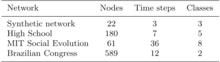
Table 1.Summary of networks used in this paper.
Network Nodes Time steps Classes
Synthetic network 22 3 3
High School 180 7 5
MIT Social Evolution 61 36 8
Brazilian Congress 589 12 2
2.2 Network data
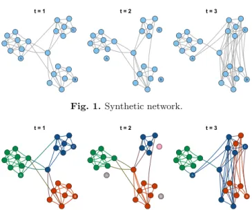
SeqMod is tested on synthetic and real networks, sum-marised in Table 1. First, as an illustrative example, we have adapted a small synthetic network from [33]. This network comprises 22 nodes and 3 time steps. The net-work has 3 clearly defined communities att= 1 but con-nections between two of them become increasingly denser att= 2 andt= 3.
We have also tested real social networks, generated from proximity data among high school students, college students and members of the Brazilian Congress. The High School network represents the interactions among 180 high school students, over a period of 7 school days [34]. Students had to wear a device that would record any face to face contact with another student that lasted at least 20 s. The results were used to generate daily net-works. The authors of the study have shown that about 91.5% of contacts made between students in this high school during the study involved students in the same class.
The third network was built from the MIT social evo-lution dataset [35], consisting of records of eighty MIT students who lived in the university dormitory during an academic year. Various types of interaction data (WiFi location, Bluetooth proximity, SMS and Calls exchanged) was collected using mobile phones that were given to the students. We selected Bluetooth proximity data to gener-ate a dynamic network of weekly snapshots for 36 weeks. We restricted our network to the students who had their dormitory sector and year of studies mapped by the re-searchers and used only the records that had a probabil-ity of at least 20% that the involved students lived on the same dormitory floor. The final network, after applying these restrictions, had 61 nodes.
The fourth network was built from a dataset of the records of the roll call votes in the Brazilian Chamber of Deputies (the lower house of the Congress)1. To construct the networks, we first selected records in the period from 2003, the first year of the current ruling party govern-ment (PT) to 2014. Duplicated entries of each congress-man were removed, results were ranked according to par-ties and records of the topmost four parpar-ties were selected. Two of these parties are in the opposition group (PSDB and DEM) while the other two are allied to the govern-ment (PT and PMDB). For every year in the records, we computed a weighted adjacency matrix based on [36] 1 The data was downloaded from https://github.com/
in which each cell represents the similarity of the votes of each pair of congressmen during that year. Unanimous vote sessions, i.e. cases where 95% of the present congress-men vote the same, were removed.
2.3 Alternative clustering methods
We compare our results with other algorithms for com-munity detection through evolutionary clustering, namely Estrangement, FacetNet and DynMOGA. The Estrang-ment algorithm [19] solves the snapshots sequentially us-ing modularity and a measure of dissimilarity between two partitions called estrangement, which is proportional to the number of intra-community edges that becomes in-ter community over time. FacetNet [16] is based on a stochastic block model for the detection of communities and a probablistic model based on Dirichlet distribution that detects the evolution of the communities. DynMOGA is a multiobjective genetic algorithm that optimizes both modularity and normalized mutual information (with re-spect to the previous time step) [20].
We also compare our method to genLouvain [37], a ro-bust algorithm with a modified version of modularity de-signed for multilayer networks. In order to obtain results that are comparable to an evolutionary clustering frame-work, we apply genLouvain sequentially at each time step, i.e. to detect the partitions for the network att1, we input the first snapshot; for the second time step, we providet1
andt2as input, and follow a similar procedure for all other ensuing time snapshots.
2.4 Adjusted rand index
In order to evaluate the accuracy of SeqMod in detect-ing the ground truth community structure, we employ the Adjusted Rand Index (ARI) metric [38], a measure of sim-ilarity between two partitions, comparing it to a null prob-abilistic model. ARI yields 1 for identical partitions and usually 0 for independent partitions, although it may also result in some negative values [39]. We used the mclust package implementation of ARI in R [40].
3 Results and discussion
3.1 Synthetic network
For illustrative purposes, we tested our model on a small synthetic network, shown in Figure1. We note three clear distinct communities (one on the left and the other two on the top, and bottom right, respectively). The two right-most communities have increasingly denser connections between them att2 and t3. We investigate whether Seq-Mod can maintain the three communities over time and under what values ofε.
If we fix ε = 0 for all time steps, the model does not consider historic information and each time step is
● ● ● ● ● ● ● ● ● ●● ● ● ● ● ● ● ● ● ● ● ● A B C t = 1 ● ● ● ● ● ● ● ● ● ●● ● ● ● ● ● ● ● ● ● ● ● A B C t = 2 ● ● ● ● ● ● ● ● ● ●● ● ● ● ● ● ● ● ● ● ● ● A B C t = 3
Fig. 1.Synthetic network.
● ● ● ● ● ● ● ● ● ●● ● ● ● ● ● ● ● ● ● ● ● A B C t = 1 ● ● ● ● ● ● ● ● ● ●● ● ● ● ● ● ● ● ● ● ● ● A B C t = 2 ● ● ● ● ● ● ● ● ● ●● ● ● ● ● ● ● ● ● ● ● ● A B C t = 3
Fig. 2. Partitions detected by SeqMod for the synthetic net-work, usingε= 0.00. ● ● ● ● ● ● ● ● ● ●● ● ● ● ● ● ● ● ● ● ● ● A B C t = 1 ● ● ● ● ● ● ● ● ● ●● ● ● ● ● ● ● ● ● ● ● ● A B C t = 2 ● ● ● ● ● ● ● ● ● ●● ● ● ● ● ● ● ● ● ● ● ● A B C t = 3
Fig. 3. Partitions detected by SeqMod for the synthetic net-work, usingε≥0.10.
solved sequentially considering only modularity. The re-sult is shown in Figure 2. At t1, three communities are detected, at t2 the network is just slightly different, now the central node is placed in the red community instead of the blue. This reflects the minor changes in this snapshot, this node changed membership because at this time step it has more connections with the red community than with the others. Att3, there are now more edges between the red and blue communities and the community structure is different from the previous time steps. The three nodes marked A, B and C on the plot either did not interact with any other node at t2 or are not present in the net-work at that time step, in our model we treat such nodes as isolated nodes. Since no historic information was taken into account, these nodes are assigned each to a singleton community at that time step.
The results are different when ε >0, Figure 3 shows the partitions detected by SeqMod for the synthetic net-work for ε ≥ 0.10. Community structure is now main-tained fromt1tot2even though the network has changed and at t3, SeqMod detects a merge between the red and blue communities. Note also that the absent nodes at t2
are maintained in their original community (fromt1). This is an advantage of the evolutionary clustering approach: it takes advantage of prior knowledge to infer the node community allocation even in the snapshot where it is not present/interacting.
● ● ● ● ● ● ● ● ● ● ● ● ● ● ● ● ● ● ● ● ● ● ● ● ● ● ● ● ● ● ● ● ● ● ● 0.4 0.6 0.8 1 2 3 4 5 6 7 Time step
Adjusted Rand Inde
x Parameter (ε) ● ● ● ● ● 0.00 0.05 0.15 0.25 0.50
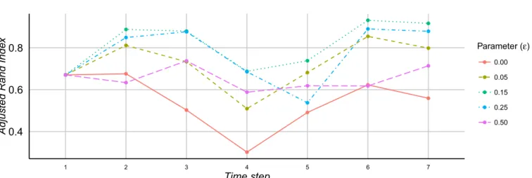
Fig. 4.High school network – the change in Adjusted Rand Index (ARI) at each time step for SeqMod depending on the value ofε.
Node A is a good example of a “promiscuous” node and its community membership is determined by the pa-rameter ε. For example, if we fix ε = 0.015 the node is assigned to the green community att1 and is kept green att2, when it is absent, but on the third time step it be-longs to the blue community since now it has more ties with that group. The desired smoothness is controlled by the user parameter.
3.2 High school network
Our first real network is a proximity network created by aggregating information on face-to-face contacts be-tween high school students. Students belong to one of five classes, each with a specific discipline programme: two MPclasses, with a focus on mathematics and physics; two PCclasses, with a focus on physics and chemistry and one PSIclass, with focus on engineering. We take these classes as our ground truth communities and we investigate how closely our model detects them. Students are more likely to interact with other members of the same class [34].
We tested the High School network with a maximum number of communities set to 10 and Figure4shows how the difference to the ground truth network (expressed by ARI) changes over time according to the value of ε. We tested ε in the range [0.00,0.50], in intervals of 0.05. At timet1, since there is no previous historic information, all test cases found the same partition but for the next time steps, all test cases for ε ≤ 0.30 have always improved ARI over the partitions withε= 0.00.
This means that by properly setting the user parame-ter, it is possible to gain more information about the true communities of a network than with a static method. Fur-thermore, our dynamic community detection method is more accurate than applying a static community detection method to the aggregated network for this example; the Louvain algorithm [41] finds a solution with ARI = 0.763, less than the average result for SeqMod using ε = 0.15 (ARI = 0.816).
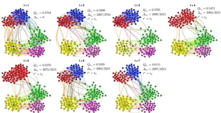
Figure 5 shows the evolution of the network commu-nity structure for ε= 0.15. Notice that duringt4 and t5
the red and blue communities are merged, they correspond to the twoMPclasses in the network, showing that stu-dents are also more likely to interact with others in similar disciplines than with the rest as previously noted by [34]. In all test cases whereε >0.05 andε <0.30, this pattern occurs to some extent at these time steps; it can also be perceived from Figure5where for these values ofε, there is drastic change in interaction patterns att4andt5(drop in ARI) that is followed by an increase in the metric for the next time steps (t6andt7). This seems to suggest that these classes were more involved in activities together dur-ing these days or even that these students are more likely to interact on Thursdays (t3) and Fridays (t4) than on Mondays (t1, t6), Tuesdays (t2,t7) and Wednesday (t3).
3.3 MIT social evolution dataset
The network built from Bluetooth proximity records from the MIT Social Evolution dataset is smaller than the pre-vious network in terms of nodes but represents a longer time period. The interactions of the students in the So-cial Evolution network are registered based on Bluetooth proximity data rather than face-to-face contacts, as in the High School network, so some of the records may actually correspond to “false interactions”. For example, if there is a record representing an interaction between students A and B, it may mean that they were in fact in different floors or room and not interacting at all. Therefore we restricted our network to those interactions with at least 20% of chance that they were in the same floor.
The dormitory sector where each student lived was re-ported to be the primary factor in defining the relation-ships between students [35], so we take the dormitory sec-tors as the ground truth communities for this network. Figure6 shows the ARI results for various values ofε.
Once again, by incorporating historic information (any 0 < ε < 0.20) the model yields results closer to the ground truth than clustering each snapshot individually. For ε = 0.05, the model improves in ARI over the re-sults for ε = 0.00 and it still adapts to some major
Fig. 5. Partitions detected for High school network by SeqMod, withε= 0.15. ● ● ● ● ● ● ● ● ● ● ● ● ● ● ● ● ● ● ● ● ● ● ● ● ● ● ● ● ● ● ● ● ● ● ● ● ● ● ● ● ● ● ● ● ● ● ● ● ● ● ● ● ● ● ● ● ● ● ● ● ● ● ● ● ● ● ● ● ● ● ● ● ● ● ● ● ● ● ● ● ● ● ● ● ● ● ● ● ● ● ● ● ● ● ● ● ● ● ● ● ● ● ● ● ● ● ● ● ● ● ● ● ● ● ● ● ● ● ● ● ● ● ● ● ● ● ● ● ● ● ● ● ● ● ● ● ● ● ● ● ● ● ● ● ● ● ● ● ● ● ● ● ● ● ● ● ● ● ● ● ● ● ● ● ● ● ● ● ● ● ● ● ● ● ● ● ● ● ● ● 0.0 0.1 0.2 0.3 0.4 1 2 3 4 5 6 7 8 9 10 11 12 13 14 15 16 17 18 19 20 21 22 23 24 25 26 27 28 29 30 31 32 33 34 35 36 Time step
Adjusted Rand Inde
x Parameter (ε) ● ● ● ● ● 0.00 0.05 0.10 0.25 0.50
Fig. 6.MIT social evolution network – the change in adjusted rand index (ARI) at each time step for SeqMod depending on the value ofε.
changes in community structure in the network. There is a pattern of decrease in ARI during the intervals
{t12−t16, t19−t21, t26−t28}, the first of them correspond to the weeks of Christmas and New Year’s Eve Holidays and the network is considerably reduced during these time steps (about 80% of students were absent). This explains why the model is more capable of matching the ground truth for relatively larger ε during the Holiday season: since the majority of the network consists of absent nodes, the community structure found previously is maintained. We also note the trade-off nature of the smoothness control in the model. For this network, whenε= 0.10 the model yields the best result in terms of matching the true classes of the students (mean ARI = 0.371) but as it can be noticed in Figure 6, when solving with ε = 0.05 the model is better at detecting the changes in the network,
ARI decreases during the holiday periods. One has to bal-ance between the current state of the network, incorpo-rating “ground truth” information sequentially, while also allowing for change. Ifεis set too large, for example 0.50, the model might incur “over-smoothing”, i.e. being unable to adapt to changes in the community structure on this period [42].
3.4 Brazilian congress voting dataset
The Brazilian Congress network consists of 589 nodes and 12 time steps. The ground truth used as validation for this dataset is the political alignment of the congressmen, based on their parties (either left-wing or right-wing). Fig-ure7shows the ARI results found by SeqMod at each time
● ● ● ● ● ● ● ● ● ● ● ● ● ● ● ● ● ● ● ● ● ● ● ● ● ● ● ● ● ● ● ● ● ● ● ● ● ● ● ● ● ● ● ● ● ● ● ● 0.05 0.10 0.15 0.20 0.25 1 2 3 4 5 6 7 8 9 10 11 12 Time step
Adjusted Rand Inde
x Parameter (ε) ● ● ● ● 0.00 0.10 0.20 0.50
Fig. 7.Brazilian congress network – the change in adjusted rand index (ARI) at each time step for SeqMod depending on the value ofε.
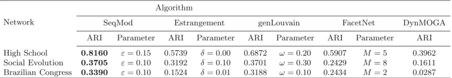
Table 2. Best results found by each algorithm and the respective parameters that has returned such results.
Network
Algorithm
SeqMod Estrangement genLouvain FacetNet DynMOGA
ARI Parameter ARI Parameter ARI Parameter ARI Parameter ARI High School 0.8160 ε= 0.15 0.5739 δ= 0.00 0.6872 ω= 0.20 0.5907 M = 5 0.3962 Social Evolution 0.3705 ε= 0.10 0.3192 δ= 0.10 0.3701 ω= 0.30 0.2429 M = 8 0.1611 Brazilian Congress 0.3390 ε= 0.10 0.1524 δ= 0.01 0.3188 ω= 0.10 0.2434 M = 2 0.0287
step for different values ofε. The best average results were found withε= 0.10 and results ontained forε= 0.20 are also favourable. Whenε= 0.50, the accuracy of the algo-rithm decreases, but is still better than when no historical information is considered (ε= 0.00).
4 Comparative analyses
We compare SeqMod with the Estrangement, FacetNet, DynMOGA and genLouvain algorithms. Since Estrange-ment and FacetNet do not output information about ab-sent nodes and ARI only compares two membership vec-tors of the same size, we have assigned each of these nodes to a unique community label for comparison purposes. The parameters were set as follows: we tested ε in the range [0.00,0.50], in intervals of 0.05 for SeqMod and the max-imum number of communities was set to 10, 10 and 4 for the High School, MIT Social Evolution and Brazilian Congress network,respectively. For the Estrangement al-gorithm, the default set of parameters defined by the au-thors (δ= 0.00,0.01,0.025,0.05) were employed, plus ad-ditional parameters (δ= 0.1,0.2, . . . ,0.5). For FacetNet a fixed number of communities should be specified, so we fixed it to to the number of communities in the ground truth for each dataset. GenLouvain was tested foromega
ranging from 0.00 to 0.50 in intervals of 0.05. Across all methods, deciding on which parameter to use for compar-ison is important, so we report the test cases that have yielded the largest average ARI (across all time steps) for each algorithm. Table2 reports the best average ARI
found by each algorithm and the parameters used to find these results.
Figure8shows the results on the High School network for the parameters reported in Table2at each time step. The algorithms seem to detect a similar pattern on the network fromt3to t5: they all show a decrease in ARI in this period and most algorithms show an increase in this metric during the last two time steps. SeqMod, however, provided the more accurate results, matching more closely the ground truth communities of this network through time (average ARI = 0.8160).
The best results for the MIT Social Evolution network are shown in Figure9. SeqMod again shows the best per-formance overall in terms of ARI with ε= 0.10 followed closely by genLouvain. As discussed previously and shown in Figure6, the results found with this parameter were the closest to the ground truth. It is noteworthy that tests with smallerεwere able to show structural changes in the network during holiday periods t13−t15 and around t20
and t27. These changes were detected by Estrangement and also by DynMOGA and FacetNet, although with less accuracy.
This fact once again highlights the existing balance between detecting the ground truth of a network and the changes in network structure, which is evident even in al-gorithms without a smoothness parameter like FacetNet and DynMOGA. If the objective is to detect changes in the network, the smoothness parameter must be set in a way that allows for more adaptation. In SeqMod, this means that ε must be set to a lower value as discussed
● ● ● ● ● ● ● 0.4 0.6 0.8 1 2 3 4 5 6 7 Time step
Adjusted Rand Inde
x Algorithm ● Seqmodε = 0.15 Estrangement δ = 0.00 genLouvain ω = 0.20 FacetNet M = 5 DynMOGA
Fig. 8.High school network – the change in adjusted rand index (ARI) at each time step for each algorithm.
● ● ● ● ● ● ● ● ● ● ● ● ● ● ● ● ● ● ● ● ● ● ● ● ● ● ● ● ● ● ● ● ● ● ● ● 0.0 0.1 0.2 0.3 0.4 1 2 3 4 5 6 7 8 9 10 11 12 13 14 15 16 17 18 19 20 21 22 23 24 25 26 27 28 29 30 31 32 33 34 35 36 Time step
Adjusted Rand Inde
x Algorithm ● Seqmodε = 0.10 Estrangement δ = 0.10 genLouvain ω = 0.30 FacetNet M = 8 DynMOGA
Fig. 9.MIT social evolution network – the change in adjusted rand index (ARI) at each time step for each algorithm.
before. Estrangement algorithm and SeqMod with ε = 0.05 exhibit the more drastic discontinuities in the network.
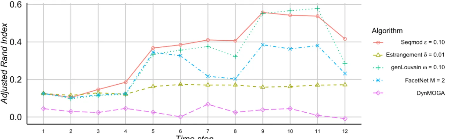
The tests with Brazilian Congress network show simi-lar results (Fig.10). SeqMod achieves the best accuracy of algorithms, followed by genLouvain. Both algorithms ex-hibit a sudden increase in ARI fromt4 tot5 and fromt8
tot9, corresponding to the years of elections and renewal of congressmen in the Chamber of Deputies in Brazil. A decrease in ARI is observed for most algorithms fromt11
tot12 and since the ground truth is the alignment of the parties, we conjecture that this change reflects the changes in political alignment of the parties due to the recent po-litical crisis in Brazil that started in 2014 when a major corruption scandal was revealed [43].
5 Conclusions
In this paper, we proposed an alternative approach to sequential clustering of evolving networks using mathe-matical programming. The proposed method is an ex-tension of our previous work to consider historic infor-mation when detecting community structure of dynamic
networks, under evolutionary clustering framework. We validated our model on dynamic networks with known ground truth communities and compared it to other meth-ods who also employ both historic information and mod-ularity optimisation.
Our model uses a different concept of similarity where a preservation coefficient allows for an intuitive under-standing of the number of vertex pairs that were main-tained in the network. We also introduce the concept of a “reference snapshot”, instead of using the immediate pre-vious time step in the historical cost, we use the prepre-vious time step with the largest modularity. The reason is that we want to maximize the ability of our model to detect the ground truth of communities through time, comparing each snapshot with a previous better defined community structure.
We have shown that our model is able to detect the ground truth of dynamic networks and changes in the network community structure. We have shown with our illustrative example that our model is able to incorpo-rate historic information to detect probable changes in the network and that it also maintains the information, shedding light on the membership of the nodes that do not interact during all time steps, i.e. that are absent or
● ● ● ● ● ● ● ● ● ● ● ● 0.0 0.2 0.4 0.6 1 2 3 4 5 6 7 8 9 10 11 12 Time step
Adjusted Rand Inde
x Algorithm ● Seqmodε = 0.10 Estrangement δ = 0.01 genLouvain ω = 0.10 FacetNet M = 2 DynMOGA
Fig. 10.Brazilian congress network – the change in adjusted rand index (ARI) at each time step for each algorithm.
isolated. Determining the desired smoothness is the main challenge of evolutionary clustering and consequently of our model, but from the results obtained in this study, we suggest a value around 0.10 and 0.15. Some methods automatically determine the parameter at each time step based on probabilistic models and statistical features of the network while algorithms like DynMOGA model this process as a multiobjective problem and hence do not re-quire any parameters, but as our tests have shown, these algorithms found poor results. We intend to improve our mathematical programming model in the future to adapt to the changes in the network without the need of pa-rameter setting, while also providing solutions of suitable quality.
Mathematical programming provides a flexible envi-ronment for modelling community detection and here we have illustrated its use for evolutionary clustering. We note that this type of modelling framework is par-ticularly adaptable and can accommodate various user requirements, one can for example specify a module al-location for determined nodes if known, one can add con-straints that change the way isolated nodes are treated or any other logical conditions necessary for a pratical ap-plication. Therefore, we believe that such approaches will prove to be popular in future network analysis method-ologies and applications.
Author contribution statement
JCS, LGP, LB, ST conceived and designed the experi-ments. JCS, LGP, LB, ST designed the computational model. JCS, LB performed the experiments. JCS gath-ered network data. JCS, LGP, LB, ST analysed the data. JCS, LB, ST, LGP wrote the paper.
JCS acknowledges funding from CAPES, Brazil (Process num-ber 13312138). ST and LGP acknowledge funding from the UK Leverhulme Trust (RPG-2012-686). We would like to thank an anonymous reviewer for helpful comments to improve our manuscript.
References
1. M. Girvan, M.E.J. Newman, Proc. Natl. Acad. Sci. USA
99, 7821 (2002)
2. R. Guimera, L.A.N. Amaral, Nature433, 895 (2005) 3. T.M. Przytycka, M. Singh, D.K. Slonim, Briefings in
Bioinformatics 11, 15 (2010)
4. T. Aynaud, J.L. Guillaume, inFifth SNA-KDD Workshop Social Network Mining and Analysis in conjunction with the 17th ACM SIGKDD International Conference on Knowledge Discovery and Data Mining – KDD 2011
(2011), Vol. 11
5. A. Lancichinetti, S. Fortunato, Sci. Rep.2, 336 (2012) 6. L. Bennett, A. Kittas, G. Muirhead, L.G. Papageorgiou,
S. Tsoka, Sci. Rep.5, 10345 (2015)
7. G. Palla, A.L. Barab´asi, T. Vicsek, Nature 446, 664 (2007)
8. C. Tantipathananandh, T. Berger-Wolf, D. Kempe, A framework for community identification in dynamic social networks, inProc. 13th ACM SIGKDD international con-ference on Knowledge discovery and data mining – KDD ’07 (ACM Press, New York, 2007), pp. 717–726
9. D.J. Fenn, M.A. Porter, M. McDonald, S. Williams, N.F. Johnson, N.S. Jones, Chaos19, 1 (2009)
10. J. Kauffman, A. Kittas, L. Bennett, S. Tsoka, PLoS ONE
9, e101357 (2014)
11. J. Sun, P.S. Yu, C. Faloutsos, in Proceedings of the 13th ACM SIGKDD international conference on Knowledge discovery and data mining(2007), pp. 687–696
12. S. Asur, S. Parthasarathy, D. Ucar, ACM Trans. Knowl. Discov. Data3, 1 (2009)
13. D. Chakrabarti, R. Kumar, A. Tomkins, Evolutionary clus-tering, inProceedings of the 12th ACM SIGKDD interna-tional conference on Knowledge discovery and data min-ing – KDD ’06(ACM Press, New York, 2006), pp. 554–560 14. Y. Chi, X. Song, D. Zhou, K. Hino, B.L. Tseng, Evolutionary spectral clustering by incorporating tempo-ral smoothness, inProceedings of the 13th ACM SIGKDD international conference on Knowledge discovery and data mining – KDD ’07 (ACM Press, New York, 2007), pp. 153–162
15. M.S. Kim, J. Han, inProceedings of the VLDB Endowment
16. Y.R. Lin, Y. Chi, S. Zhu, H. Sundaram, B.L. Tseng, ACM Trans. Knowl. Discov. Data3, 1 (2009)
17. N.P. Nguyen, T.N. Dinh, Y. Xuan, M.T. Thai, Adaptive algorithms for detecting community structure in dynamic social networks, inProceedings IEEE INFOCOM (2011), pp. 2282–2290
18. R. G¨orke, P. Maillard, A. Schumm, C. Staudt, D. Wagner, J. Exp. Algorithmics18, 1 (2011)
19. V. Kawadia, S. Sreenivasan, Sci. Rep.2, 794 (2012) 20. F. Folino, C. Pizzuti, IEEE Trans. Knowl. Data Eng.26,
1838 (2014)
21. N.P. Nguyen, T.N. Dinh, Y. Shen, M.T. Thai, PloS ONE
9, e91431 (2014)
22. G. Xu, S. Tsoka, L.G. Papageorgiou, Eur. Phys. J. B60, 231 (2007)
23. G. Agarwal, D. Kempe, Eur. Phys. J. B66, 409 (2008) 24. G. Xu, L. Bennett, L.G. Papageorgiou, S. Tsoka,
Algorithms Mol. Biol.5, 1 (2010)
25. D. Aloise, S. Cafieri, G. Caporossi, P. Hansen, S. Perron, L. Liberti, Phys. Rev. E82, 046112 (2010)
26. S. Cafieri, P. Hansen, L. Liberti, Phys. Rev. E83, 056105 (2011)
27. L. Bennett, S. Liu, L.G. Papageorgiou, S. Tsoka, Adv. Complex Syst.15, 1150023 (2012)
28. D. Aloise, G. Caporossi, P. Hansen, L. Liberti, S. Perron, M. Ruiz, Modularity maximization in networks by vari-able neighborhood search, in Proceedings of the 10th DIMACS implementation challenge workshop (American Mathematical Society (AMS), Atlanta, 2013), pp. 113–127 29. L. Bennett, A. Kittas, S. Liu, L.G. Papageorgiou, S. Tsoka,
PLoS ONE9, e112821 (2014)
30. M.E.J. Newman, M. Girvan, Phys. Rev. E 69, 026113 (2004)
31. U. Brandes, D. Delling, M. Gaertler, R. Gorke, M. Hoefer, Z. Nikoloski, D. Wagner, IEEE Trans. Knowl. Data Eng.
20, 172 (2008)
32. R.E. Rosenthal,GAMS A User’s Guide(2014),www.gams. com/mccarl/mccarlhtml/
33. D.S. Bassett, M.A. Porter, N.F. Wymbs, S.T. Grafton, J.M. Carlson, P.J. Mucha, Chaos23, 013142 (2013) 34. J. Fournet, A. Barrat, PloS ONE9, e107878 (2014) 35. W. Dong, B. Lepri, A. Pentland, Modeling the co-evolution
of behaviors and social relationships using mobile phone data, in Proceedings of the 10th International Conference on Mobile and Ubiquitous Multimedia – MUM ’11 (ACM Press, New York, 2011), pp. 134–143
36. V. Baptista, F. Brito, J. Brasileiro, A.N. Duarte, E.P. Bezerra, F. Almeida, P. Lima, S. Guimaraes, Uma fer-ramenta para analisar mudan¸cas na coes˜ao entre parla-mentares em vota¸c˜oes nominais, inIII Brazilian Workshop on Social Network Analysis and Mining(2014), pp. 1–7 37. P.J. Mucha, T. Richardson, K. Macon, M.A. Porter, J.P.
Onnela, Science328, 876 (2010)
38. L. Hubert, P. Arabie, J. Classification2, 193 (1985) 39. M. Meil, J. Multivariate Anal.98, 873 (2007)
40. C. Fraley, A.E. Raftery, T.B. Murphy, L. Scrucca, mclust Version 4 for R: Normal Mixture Modeling for Model-Based Clustering, Classification, and Density Estimation, Technical Report No. 597 (2012)
41. V.D. Blondel, J.L. Guillaume, R. Lambiotte, E. Lefebvre, J. Stat. Mech.: Theor. Exp.2008, P10008 (2008)
42. K.S. Xu, M. Kliger, A.O. Hero, Evolutionary spectral clustering with adaptive forgetting factor, in 2010 IEEE International Conference on Acoustics, Speech and Signal Processing (IEEE, 2010), pp. 2174–2177
43. The Guardian, Petrobras scandal: Brazilian oil execu-tives among 35 charged,http://goo.gl/fqUaqY, accessed: 2015-10-06
Open Access This is an open access article distributed under the terms of the Creative Commons Attribution License (http://creativecommons.org/licenses/by/4.0), which permits unrestricted use, distribution, and reproduction in any medium, provided the original work is properly cited.