Survey sampling targeted inference
Antoine Chambaz, Emilien Joly, Xavier Mary
To cite this version:
Antoine Chambaz, Emilien Joly, Xavier Mary. Survey sampling targeted inference. 2016.
<
hal-01359219
>
HAL Id: hal-01359219
https://hal.archives-ouvertes.fr/hal-01359219
Submitted on 2 Sep 2016
HAL
is a multi-disciplinary open access
archive for the deposit and dissemination of
sci-entific research documents, whether they are
pub-lished or not.
The documents may come from
teaching and research institutions in France or
abroad, or from public or private research centers.
L’archive ouverte pluridisciplinaire
HAL
, est
destin´
ee au d´
epˆ
ot et `
a la diffusion de documents
scientifiques de niveau recherche, publi´
es ou non,
´
emanant des ´
etablissements d’enseignement et de
recherche fran¸cais ou ´
etrangers, des laboratoires
publics ou priv´
es.
Survey sampling targeted inference
Antoine Chambaz1,2,3, Emilien Joly1, and Xavier Mary1 1 Modal’X, Universit´e Paris Nanterre2 Division of Biostatistics, School of Public Health, UC Berkeley 3 MAP5 (UMR CMRS 8145), Universit´e Paris Descartes
1 Introduction
Consider the following situation: we wish to build a confidence interval (CI) for a real-valued pathwise differentiable parameterΨ evaluated at a lawP0,ψ0 ≡Ψ(P0), from a data set O1, . . . , ON of independent random variables drawn from P0 but, as is often the case nowadays, N is so large that we will not be able to use all data. To overcome this computational hurdle, we decide(i)to selectnamongN observations randomly with unequal probabilities and(ii)to adapt targeted minimum loss inference from the smaller data set that results from the selection. First explored in (Bertail et al.,2016a), our approach is an alternative to the so called “online targeted learning” developed byvan der Laan and Lendle(2014).
The selection ofnamongN observations will be the random outcome of a survey sampling design. From now on, we assume that each observationOi is summarized byVi, a low-dimensional random variable, and thatV1, . . . , VN are all observed. We will draw advantage fromV1, . . . , VN to adjust the probability that each
Oi be sampled. We will develop two examples of survey sampling designs: Sampford’s and determinantal sampling designs. Also known as rejective sampling design based on Poisson sampling with unequal inclusion probabilities, Sampford’s sampling design is a particular case of sampling without replacement (Hanif and Brewer, 1980). It has been thoroughly studied since the publication of the seminal articles (Hajek, 1964;
Sampford,1967). Recently introduced in sampling theory byLoonis and Mary (2015), determinantal sam-pling design benefits from a rich literature on determinantal point processes (Macchi, 1975; Lyons, 2003;
Hough et al.,2006).
The manuscript is organized as follows. Section 2 presents the general template for targeted inference from large data sets by survey sampling. Section 3 introduces and discusses the two examples of survey sampling designs mentioned above. Section 4 addresses their optimization in terms of minimization of the asymptotic variance of the targeted estimator resulting from their use. Section5develops an example, that of the inference of a variable importance measure of a continuous exposure. Section6 presents a simulation study illustrating the implementation of the general template in the example. Finally, Section7gathers some elements of proof.
2 Template for targeted inference from large data sets by survey sampling
This section presents a template for carrying out targeted inference from large data sets by survey sampling. Section 2.1formalizes survey sampling. Section 2.2 quickly describes the construction of the targeted min-imum loss estimator (TMLE, which also stands for targeted minmin-imum loss estimation) based on a survey sample and states a central limit theorem (CLT) which enables the construction of CIs of given asymptotic level. The CLT relies on general assumptions typical of empirical processes theory. Section3discusses them in the contexts of the Sampford’s and determinantal survey sampling designs.Throughout the manuscript, we denote µf ≡ R
f dµ and kfk2,µ ≡ (µf2)1/2 for any measure µ and functionf (measurable and integrable with respect toµ).
2.1 Retrieving the observations by survey sampling
As explained in introduction, the first step of the inference procedure is the random selection without replace-ment ofnamongN observations. The survey sample sizenis set beforehand. Down to earth computational considerations (how many data can the package handle?; how much time are we willing to wait for the results of inference?) typically drive its choice.
Our analysis is asymptotic: we assume that N goes to infinity and thatngoes to infinity asN does, in such a way that the ration/N go to 0. How n depends on N may or may not need to be described more precisely. The results of this manuscript could be extended to the case thatnis random and satisfies these two conditions almost surely (with respect to the law of the sampling design; more details to follow).
The random selection of namong N observations takes the form of a vectorη ≡(η1, . . . , ηN) of binary random variables where, for each 1≤i≤N, Oi is selected if and only ifηi equals 1. The conditional joint distribution of η given O1, . . . , ON is the survey sampling design. By construction, it coincides with the conditional joint distribution of η given the summary measuresV1, . . . , Vn which, contrary to O1, . . . , ON, are all observed at the beginning of the study.
We denotePsa generic conditional joint distribution ofηgivenO
1, . . . , On(the superscript “s” stands for “survey”). The first order inclusion probabilities are the (conditional marginal) probabilitiesπi≡Ps(ηi= 1) for 1 ≤ i ≤ N. In case they are equal, the sampling design is said equally weighted. The second order inclusion probabilities are the (conditional joint) probabilitiesπij ≡Ps(ηi = 1, ηj = 1) = Ps(ηiηj = 1) for 1≤i6=j ≤N. The Horvitz-Thompson empirical measure
PnHT≡ 1 N N X i=1 ηi πi Dirac(Oi) (0.1)
takes up the role that the empirical measure PN ≡N−1P N
i=1Dirac(Oi) would play if we had access to it. The former is an unbiased estimator of the latter in the sense that, for any functionf ofO drawn fromP0,
EPsPnHTf=PNf.
A CLT may hold for√n(PHT
n −PN)f(conditionally onO1, . . . , ON). Whether it does or not notably depends on the asymptotic behavior of VarPsPnHTf. In general, it holds that
VarPsPnHTf= 1 N2 N X i=1 1 πi −1 f2(Oi) + 1 N2 X 1≤i6=j≤N π ij πiπj −1 f(Oi)f(Oj). (0.2)
Sections 3 and 4 focus on the specific examples of the Sampford and determinantal survey sampling designs. The choice of the sampling design affects the limit variance of the TMLE. For the time being, we do not characterize further the survey sampling design.
2.2 CLT on the TMLE and resulting confidence intervals
Constructing the TMLE.We begin with a minor twist. We assume that the real-valued pathwise differ-entiable parameter of interestΨ, originally seen as a real-valued mapping on the set of probability measures on O equipped with the Borel σ-field, can be extended to a real-valued mapping on the set M of finite measures onO equipped with the Borelσ-field. Moreover, we assume that the extension can be performed in such a way that the pathwise differentiability of Ψ is preserved: for eachP ∈M(not necessarily a prob-ability measure), there exists an influence function D(P)∈L20(P) (the set of measurable functionsf onO
satisfyingP f = 0 andP f2 finite) such that, for all boundeds∈L02(P) with ksk∞ >0, if we characterize
P∈Mby setting dP/dP = 1 +s (all∈Rwith||<ksk−1∞), then 7→Ψ(P) is differentiable at= 0 with a derivative equal toP sD(P). This is not asking much, as the example developed in Section5illustrates.
Suppose that we have constructed Pn∗∈Mtargeted toψ0 in the sense that
PnHTD(Pn∗) =oP(1/ √
n). (0.3)
The TMLE is the substitution estimatorψ∗n≡Ψ(Pn∗).
Central limit theorem and CIs. The CLT hinges on three assumptions. We suppose the existence of F ⊂ {D(P) :P ∈M}such that
A1. The empirical process√n(PHT
n −P0) converges in law in`∞(F) to a zero-mean Gaussian process with covariance functionΣh.
A2. WithP0-probability tending to one,D(Pn∗)∈ F, and there existsf1∈ Fsuch thatkD(Pn∗)−f1k2,P0= oP(1). Moreover, one knows a conservative estimatorσ2n ofσ
2
1≡Σh(f1, f1). Conservative estimation ofσ2
1is not as easy as one might think at first sight. For instance, it is not guaranteed in general that the substitution estimator
ˆ
σn2≡PnHTD(Pn∗)2h−1 (0.4) estimates conservativelyσ2
1. Relying on the non-parametric bootstrap is not a solution either in general. The third assumption guarantees that a second-order term in an expansion of ψ∗
n =Ψ(Pn∗) aroundP0 is indeed of second order:
A3. There exists a real-valued random variable γn converging in probability to γ1 6= 1 and such that
γn(ψ∗n −ψ0) + [ψ0−ψn∗ −P0D(Pn∗)] = oP(1/ √
n). Moreover, one knows an estimator Γn such that
Γn−γn=oP(1).
The introduction of the termγn(ψn∗−ψ0) inA3gives some flexibility. This proves useful sometimes, as for instance in the example developed in Section 5. If γn = 0, then the main condition inA3 reduces to the classicalψ0−ψ∗n−P0D(Pn∗) =oP(1/
√
n).
AssumptionsA1,A2andA3are variations on the assumptions typically made in the asymptotic analysis of TMLEs. They allow to derive the following CLT, whose proof is sketched in Section 7.1. Setα∈ (0,1) and denoteξ1−α/2 the (1−α/2)-quantile of the standard normal distribution.
Proposition 0.1.Under A1,A2andA3,(1−γn) √
n(ψ∗
n−ψ0)converges in law to the centered Gaussian
distribution with varianceσ2
1. Consequently, " ψn∗±ξ1−α/2 p σ2 n (1−Γn) √ n # (0.5)
is a confidence interval forψ0 with asymptotic coverage no less than(1−α).
Resorting to survey sampling thus makes it possible to construct a CI for ψ0. It is through σn2 that the width of CI (0.5) depends on the survey sampling design and more precisely on the covariance function in A1. In this regard, Sections3and4 will show that all survey sampling designs are not equal. In particular, simple random sampling (selectingnamongN observations without replacement and with equal weights) is suboptimal.
3 Survey sampling designs and assumption A1
This section introduces two examples of survey sampling designs and discusses A1in their respective con-texts.
3.1 Sampford’s survey sampling design
DenoteVthe space whereV drawn fromP0takes its values and lethbe a (measurable) function mappingV toR+, chosen by us in such a way thathbe bounded away from 0 and P0h= 1. For each 1≤i≤N, define
pi≡
nh(Vi)
N .
Let PsP be characterized by the fact that, under PsP, η is distributed from the conditional law of (ε1, . . . , εN) given P
N
i=1εi = n when ε1, . . . , εN are independently sampled from Bernoulli laws with pa-rametersp1, . . . , pN, respectively (we recall that this statement is conditional on O1, . . . , ON). This survey sampling design is an instance of Sampford’s survey sampling design. It is also called rejective sampling design based on Poisson (hence the superscript “P” in PsP) sampling with unequal inclusion probabilities (unequal as soon ashis not constant).
By (Bertail et al., 2016a, Theorem 2), which builds upon (Bertail et al.,2016b), assumption A1is met when using of Sampford’s survey sampling designPsP provided thatF, the class introduced in Section2.2, is not too complex: this is the message of Proposition0.2below.
Proposition 0.2.Assume thatF is separable (for instance, countable), that it admits an envelope function such that the corresponding uniform entropy integral be finite (see Condition (2.1.7) in van der Vaart and Wellner, 1996), and that P0f2h−1 is finite for all f ∈ F. Then A1 holds when using Sampford’s survey
sampling designPsP with a covariance function ΣP
h given by Σ
P
h(f, g)≡P0f gh−1.
The conclusions of Proposition 0.2still hold under the same conditions when substituting 1 N N X i=1 ηi pi Dirac(Oi) = 1 n N X i=1 ηi h(Vi) Dirac(Oi) (0.6)
for PnHT. It is thus unnecessary to compute the first order inclusion probabilities of Sampford’s survey sampling design, which differ from p1, . . . , pN whenh is not constant, and the targeting of Pn∗ ∈M to ψ0 can be achieved by ensuringn−1PN
i=1ηiD(Pn∗)(Oi)h−1(Vi) =oP(1/ √
n) instead of (0.3). 3.2 Determinantal survey sampling design
A minimalist introduction.Determinantal survey sampling designs are built upon determinantal point processes. LetK be a N×N Hermitian matrix whose eigenvalues belong to [0,1]. It happens that the set of equalities: for allI⊂ {1, . . . , N},
X
I0⊃I
Ps(I0) = det(K|I), (0.7)
uniquely characterizes the determinantal survey sampling designPsK, a probability measure on the powerset of{1, . . . , N}. Here,K|I denotes the Hermitian matrix derived fromKby keeping only its rows and columns indexed by the elements ofI.
The first and second order inclusion probabilities of PsK characterized by (0.7) are easily derived from the entries of K: for all 1 ≤ i 6= j ≤ N, if holds that πi = det(K|{i}) = Kii and πij = det(K|{i,j}) =
Kii×Kjj− |Kij|2. Furthermore, draws fromPsK are of fixed size if and only if the eigenvalues ofKbelong to{0,1}, in which caseK is a projection matrix and the fixed size equals the trace ofK. From now on, we focus on this case.
If the first order inclusion probabilities are all positive then, for any bounded function f of O drawn fromP0,PnHTf−EPsKPnHTfsatisfies a concentration inequality (Pemantle and Peres,2014, Theorem 3.1;
see also (0.20) in our Section7.3). Moreover, iff meets the so called Soshnikov conditions (0.17), (0.18) and (0.19), then √n(PHT
n −PN)f satisfies a CLT (Soshnikov, 2000). These two remarkable properties are the building blocks of Proposition0.3below. LetF0 be defined asF deprived of its elements which depend on
Proposition 0.3.Assume that F0 is countable, uniformly bounded, and that its bracketing entropy with
respect to the supremum norm is finite (see the condition preceding Condition (2.1.7) in van der Vaart and Wellner,1996). Assume moreover that, for every f ∈ F0,nVar
PsK PHT n f >0 converges inP0-probability
to a positive number and f meets the Soshnikov conditions (0.17), (0.18), (0.19) P0-almost surely. Then A1 holds with F0 substituted for F when using any fixed-size determinantal survey sampling design PsK,
provided that its first order inclusion probabilities are bounded away from 0 uniformly inN. The covariance function is defined as a limit with no closed-form expression in general.
The message of Proposition0.3 is the following: if theF0 is not too complex, and ifn/N goes to 0 suf-ficiently slowly, thenA1is met withF0 substituted forF when using most determinantal survey sampling designs PsK. The proof of Proposition 0.3 is sketched in Section 7.3. The condition on the ratio n/N is included implicitly in the assumption that the elements of F0 satisfy the Soshnikov conditions P0-almost surely. We elaborate further on this issue in Proposition0.4below.
We wish to follow the same strategy as in Section3.1,i.e., to define possibly unequal first order inclusion probabilities depending on V1, . . . , VN. There exists an algorithm to both construct and sample from a fixed-size determinantal survey sampling design with given first order inclusion probabilities (Loonis and Mary, 2015). Unfortunately, its computational burden is considerable for both tasks in general, especially in the context of large data sets (N large). In addition, the second set of conditions on F0 (and not F) in Proposition 0.3 would typically be very demanding for the yielded determinantal survey sampling design. Moreover, computing the limit variance of the TMLE resulting from its use would be difficult, and its inference would typically be achieved through the use of a very conservative estimator.
These difficulties can be overcome by focusing on V-stratified determinantal survey sampling designs equally weighted on eachV-stratum.
V-stratified determinantal sampling equally weighted on each V-stratum. We now consider the case that V drawn from P0 takes finitely many different values. To alleviate notation, we assume without loss of generality thatV ≡ {1, . . . , ν}and thatO1, . . . , ON are ordered by values of V1, . . . , VN.
Let hbe a function mappingV to R∗+ such thatPNh=N−1P N
i=1h(Vi) = 1. We will hide and neglect notation-wise the dependency ofhonV1, . . . , VN due to the normalizationPNh= 1. In the limit,hdoes not depend on the summary measures anymore: by the strong law of large numbers,PNhconvergesP0-almost surely toP0h, revealing that conditionPNh= 1 is similar to its counterpartP0h= 1 from Section 3.1. For each 1≤i≤N, define
πi ≡
nh(Vi)
N .
Similar to the proportionsp1, . . . , pN used in Section3.1to characterize a Sampford survey sampling design,
π1, . . . , πN are the exact (as opposed to approximate) first order inclusion probabilities that we choose for our determinantal survey sampling design. Its complete characterization now boils down to elaborating aN×N
Hermitian matrixΠ withπ1, . . . , πN as diagonal elements and eigenvalues in{0,1}. SinceP N
i=1πi =n, the resulting determinantal survey sampling design will be of fixed sizen.
For simplicity, we elaborateΠ under the form of a block matrix with zero matrices as off-diagonal blocks and make each of theν diagonal blocks be a projection matrix featuring the prescribed diagonal elements. This last step is easy provided thatnv≡P
N
i=1πi1{Vi=v} is an integer dividingNv≡P N
i=11{Vi=v}. In that case, the projection matrix can be a block matrix consisting ofn2
vsquare matrices of sizeNv/nv×Nv/nv, with zero off-diagonal blocks and diagonal blocks having all their entries equal ton−1v . Otherwise, we may rely on an algorithm to derive the desired projection matrix.
The determinantal survey sampling design PsΠ encoded by Π (hence the superscript “Π”) is said V -stratified and equally weighted on eachV-stratum. It randomly selects a deterministic numbernv of obser-vations from the stratum whereV =v, for each 1≤v≤ν. Sampling from it makes it possible to derive the next result, proven in Section7.2: for any functionf ofOdrawn fromP0,
EP0 VarPsΠ PnHTf = 1 nEP0 VarP0[f(O)|V]h −1(V) − 1 NEP0[VarP0[f(O)|V]]. (0.8)
Equality (0.8) is instrumental in deriving the following corollary to Proposition0.3, whose proof is sketched in Section7.3.
Proposition 0.4.Let us impose thatnis chosen in such a way thatN/n=o((N2/n))for all >0. This is
the case ifn≡N/loga(N)for somea >0, for instance. Assume thatF is separable (for instance, countable) and that its bracketing entropy with respect to the supremum norm is finite (see the condition preceding Condition (2.1.7) in van der Vaart and Wellner, 1996). Then A1 holds when using the V-stratified and equally weighted on each V-stratum determinantal survey sampling design PsΠ with a covariance function
ΣΠ h given by ΣhΠ(f, g) = EP0 CovP0[f(O)g(O)|V]h −1(V) .
Note thatΣhΠ(f, f) = 0 for everyf ∈ F which depends onOthroughV only. Actually, for such a function, √ n(PHT n −P0)f = √ n(PN −P0)f =OP( p
n/N) =oP(1). Moreover, for everyf ∈ F, combining (0.8) and equality EPsΠPnHTf=PNf readily implies
VarP0PsΠ √ n(PnHT−P0)f =ΣhΠ(f, f) + n N VarP0[f(O)]−EP0[VarP0[f(O)|V]] . (0.9) Proved in Section7.2, (0.9) relates the exact variance of√n(PHT
n −P0)f with the limit variance ΣhΠ(f, f), showing that their difference is upper-bounded by aO(n/N) =o(1)-expression.
It is an open question to determine whether or not the extra condition on howndepends onN could be relaxed or even given up by proving directly a functional CLT for√n(PnHT−P0). By “directly”, we mean without building up on functional CLTs conditional on the observations, and managing to go around the Soshnikov conditions. This route was followed to prove (Bertail et al.,2016a, Theorem 2).
Sobolev classes are known to have finite bracketing entropy with respect to the supremum norm (van der Vaart,1998, Example 19.10). The fact that the bracketing entropy is meant relative to the supremum norm instead of theL2(P
0)-norm is a little frustrating, though. Indeed, a bracketing entropy condition relative to the latter would have allowed a larger variety of classes. The supremum norm comes from the concentration inequality (Pemantle and Peres, 2014, Theorem 3.1). Perhaps the aforementioned direct proof might also allow to replace it with theL2(P
0)-norm. The covariance functions ΣP
h and Σ Π
h in Propositions0.2 and Proposition 0.4 differ. In particular, for everyf ∈ F, ΣhP(f, f) = EP0 EP0 f2(O)|V h−1(V) ≥EP0 VarP0[f(O)|V]h −1(V) =ΣhΠ(f, f) (0.10) (using the same hon both sides of (0.10) is allowed because, in the limit, conditionPNh= 1 is similar to conditionP0h= 1). Consequently,PsΠis more efficient thanPsPwhenVis finite in the sense that whichever functionhP is used to definePsP, it is always possible to choose functionhΠ to definePsΠ in such a way thatΣP
hP(f, f)≥Σ
Π
hΠ(f, f) for everyf ∈ F.
4 Optimizing the survey sampling designs
This section discusses the optimization of functions hP and hΠ used to define the first order inclusion probabilities of the survey sampling designsPsP and PsΠ that we developed in Sections 3.1 and3.2. The optimization is relative to the asymptotic variance of the TMLE,ΣhP(f1, f1) orΣhΠ(f1, f1), respectively.
In light of (0.10), letf2P andf2Π be the functions fromV toR+ given by
f2P(V)≡ q EP0[f 2 1(O)|V] and f Π 2 (V)≡ p VarP0[f1(O)|V]. (0.11)
Then (0.10) shows in particular that ΣP
h(f1, f1) = P0(f2P)2h−1 is always larger than ΣhΠ(f1, f1) =
P0(f2Π)
2h−1. Now, withf
2 equal to eitherf2P orf
Π
P0(f2)2h−1×P0h≥(P0f2) 2
,
where equality holds if and only ifhis proportional tof2. In the case ofPsP, hsatisfies P
0h= 1. Therefore, the optimalhand corresponding optimal asymptotic variance of the TMLE are
hP≡f2P/P0f2P and Σ P
hP(f1, f1) = P0f2P
2
. (0.12)
In the case ofPsΠ,hsatisfiesPNh= 1 and P0h= 1 in the limit. By analogy with (0.12), the optimalh and corresponding optimal asymptotic variance of the TMLE are
hΠ ≡f2Π/P0f2Π and Σ
Π
hΠ(f1, f1) = P0f2Π
2
. (0.13)
5 Example: variable importance measure of a continuous exposure
We illustrate our template for survey sampling targeted learning with the inference of a variable importance measure of a continuous exposure. In this example, the ith observation Oi writes (Wi, Ai, Yi)∈ O ≡ W × A ×[0,1]. Here,Wi ∈ W is the ith context,Ai ∈ A is theith exposure andYi ∈[0,1] is the ith outcome. Exposures take their values in A 30, a bounded subset ofRcontaining 0, which serves as a reference level
of exposure. Typically, in biostatistics or epidemiology,Wi could be the baseline covariate describing theith subject,Ai could describe her assignment (e.g., a dose-level) or her level of exposure, andYicould quantify her biological response.
Section5.1presents and analyzes the parameter of interest. Section5.2discusses the construction of the corresponding TMLE.
5.1 Preliminaries
For each finite measure P on O equipped with the Borel σ-field, we denote PW, PA|W and PY|A,W the marginal measures of W and conditional measures of A and Y given W and (A, W), respectively. (The conditional measure PA|W is P(O) times the conditional distribution of A given W under the probability distributionP/P(O). The conditional measurePY|A,W is defined analogously.) Moreover, for each (w, a)∈ W × A, we introduce and denote gP(0|w) ≡ PA|W=w({0}) and QP(a, w) ≡
R
[0,1]ydPY|A=a,W=w(y). In particular ifP(O) = 1, then gP(0|W) =P(A= 0|W) is the conditional probability that the exposure equal the reference value 0 and QP(A, W) = EP[Y|A, W] is the conditional expectation of the response given exposure and context.
We assume that P0,A|W(A 6= 0|W)> 0 P0,W-almost surely and the existence of a constant c(P0) > 0 such thatgP(0|W)≥c(P0)P0,W-almost surely. Introduced in (Chambaz et al.,2012;Chambaz and Neuvial,
2015), the true parameter of interest is
ψc0≡arg min β∈R EP0 h (Y −EP0[Y|A= 0, W]−βA) 2i = arg min β∈R EP0 h (EP0[Y|A, W]−EP0[Y|A= 0, W]−βA) 2i
(the superscript “c” stands for “continuous”).
In the context of this example, Mstands for the set of finite measuresP onOequipped with the Borel
σ-field such that there exists a constant c(P) > 0 guaranteeing that the marginal measure of {w ∈ W :
PA|W=w(A \ {0}) > 0 andPA|W=w({0}) ≥ c(P)} under PW equals P(O). In particular, P0 ∈ M by the above assumption. We seeψ0c as the value atP0 of the functionalΨc characterized overMby
Ψc(P)≡arg min β∈R
Z
A×W
By (Chambaz et al., 2012, Proposition 1), for eachP ∈M, Ψc(P) = R A×Wa(QP(a, w)−QP(0, w))dPA|W=w(a)dPW(w) R A×Wa2dPA|W=w(a)dPW(w) . IfP is adistribution, then Ψc(P) =EP[A(QP(A, W)−QP(0, W))] EP[A2] .
For clarity, we defineµP(w)≡
R AadPA|W=w(a) andζ2(P)≡ R A×Wa 2dP A|W=w(a)dPW(w) for allP ∈M, (w, a)∈ W × A. IfP(O) = 1, then µP(W) = EP[A|W] and ζ2(P) = EP A2
. Adapting (Chambaz et al.,
2012, Proposition 1) yields thatΨcis pathwise differentiable with influence curveDc(P)≡Dc
1(P) +Dc2(P)∈ L2 0(P), ζ2(P)D1c(P)(O)≡A(QP(A, W)−QP(0, W)−AΨc(P)), ζ2(P)D2c(P)(O)≡(Y −QP(A, W)) A−µP(W)1{A= 0} gP(0|W)
(allP∈M). Let nowRc:M2→
Rbe given by
Rc(P, P0)≡Ψc(P0)−Ψc(P)−(P0−P)Dc(P) ≡Ψc(P0)−Ψc(P)−P0Dc(P).
In light ofA3, ψ0−ψn∗−P0Dc(Pn∗) =Rc(Pn∗, P0). Adapting the last step of the proof of (Chambaz et al.,
2012, Proposition 1) yields that, for everyP, P0∈M, Rc(P, P0) = 1−ζ 2(P0) ζ2(P) (Ψc(P0)−Ψc(P)) + 1 ζ2(P)P 0 (QP0(0,·)−QP(0,·)) µP0 −µP gP0(0|·) gP(0|·) . (0.14)
We will use this equality to derive an easy to interpret sufficient condition forA3to hold.
5.2 Construction of the TMLE
Let Qw, Mw and Gw be three user-supplied classes of functions mapping A × W, W and W to [0,1], respectively. We first estimateQP0,µP0 andgP0 withQn andµn andgn built uponP
HT
n ,Qw,Mw andGw. For instance, one could simply minimize (weighted) empirical risks and define
Qn≡argmin Q∈Qw PnHT`(Y, Q(A, W)), µn≡argmin µ∈Mw PnHT`(A, µ(W)), gn≡argmin g∈Gw PnHT`(1{A= 0}, g(0|W))
(assuming that the argmins exist). Alternatively, one could prefer minimizing cross-validated (weighted) empirical risks. One then should keep in mind that the observations are dependent, because of the selection process by survey sampling. We also estimate the marginal distribution P0,W of W under P0 with Pn,WHT , defined as in (0.1) with Wi substituted forOi, and the real-valued parameter ζ2(P0) with ζ2(Pn,XHT) where
Pn,XHT is defined as in (0.1) withXi substituted forOi. Let P0
n be a measure such that QP0
n = Qn, µPn0 = µn, gPn0 =gn, ζ
2(P0
n) =ζ2(Pn,XHT), Pn,W0 = Pn,WHT ,
see (Chambaz et al., 2012, Lemma 5) for a computationally efficient choice. Then the initial estimator
Ψb(Pn0) ofψb0 can be computed with high accuracy by Monte-Carlo. It suffices to sample a large numberB (sayB= 107) of independent (A(b), W(b)) by(i)samplingW(b) fromP0
n,W =P
HT
n,W then(ii)samplingA
(b) from the conditional distribution ofA givenW =W(b) under P0
n repeatedly for b= 1, . . . , B and to make the approximation Ψc(Pn0)≈ B−1PB b=1A (b)(Q n(A(b), W(b))−Qn(0, W(b))) ζ2(P0 n) .
We now target the inference procedure and bendP0
n into Pn∗ satisfying (0.3) withDc substituted forD. We proceed iteratively. Suppose thatPk
n has been constructed for some k ≥0. We fluctuate Pnk with the one-dimensional parametric model{Pk
n() :∈R, 2≤c(Pnk)/kDc(Pnk)k∞} characterized bydPnk()/dPnk= 1 +Dc(Pk
n). Lemma 1 in (Chambaz et al.,2012) shows how QPk
n(), µPnk(), gPnk(),ζ
2(Pk
n()) andPn,Wk () depart from their counterparts at= 0. The optimal move along the fluctuation is indexed by
kn ≡arg max
PnHTlog 1 +Dc(Pnk)
,
i.e., the maximum likelihood estimator of. Note that the random function7→ PHT
n log(1 +Dc(Pnk)) is strictly concave. The optimal move results in the (k+ 1)-th update ofP0
n,Pnk+1≡Pnk(kn). There is no guarantee that a Pk+1
n will coincide with its predecessor Pnk. We assume that the iterative updating procedure converges (ink) in the sense that, for kn large enough, PnHTD
c(Pkn
n ) =oP(1/ √
n). We set Pn∗ ≡ Pkn
n . It is actually possible to come up with a one-step updating procedure (i.e., an updating procedure such thatPnk=Pnk+1for allk≥1) by relying on universally least favorable models (van der Laan,
2016). We adopt this multi-step updating procedure for simplicity.
We can assume without loss of generality that we can sampleA conditionally onW from Pn∗. The final estimator is computed with high accuracy likeΨc(P0
n) previously: withQ∗n≡QP∗
n, we sampleBindependent
(A(b), W(b)) by(i)samplingW(b) fromP∗
n,W then(ii) samplingA
(b) from the conditional distribution ofA givenW =W(b) underP∗
n repeatedly forb= 1, . . . , B and make the approximation
ψn∗ ≡Ψc(Pn∗)≈B −1PB b=1A (b)(Q∗ n(A(b), W(b))−Q∗n(0, W(b))) ζ2(P∗ n) .
To conclude this section, let us use (0.14) to derive an easy to interpret sufficient condition for A3 to hold. If we introduce γn ≡1− ζ2(P0) ζ2(P∗ n) and Γn ≡1− ζn2(P0) ζ2 n(Pn∗) where ζ2
n(P0) and ζn2(Pn∗) estimate ζ2(P0) and ζ2(Pn∗), then A3 is met provided thatζ2(Pn∗) converge in probability to a finite real number such thatγ16= 1 and
1 ζ2(P∗ n) P0 (QP0(0,·)−QPn∗(0,·)) µP0−µPn∗ gP0(0|·) gP∗ n(0|·) =oP(1/ √ n).
Through the product, we draw advantage of the synergistic convergences of QP∗
n(0,·) to QP0(0,·) and
(µP∗
n, gPn∗) to (µP0, gP0) (by the Cauchy-Schwarz inequality for example).
The next section illustrates further this example of application of our survey sampling targeted learning methodology with a simulation study.
6 Simulation study
Section6.1presents the setting of the simulation study, which illustrates the example developed in Section5 in three related but different scenarios. Section6.2summarizes its results and comments on them.
6.1 Setting
We consider three data-generating distributionsP0,1,P0,2 andP0,3 of a data-structure O= (W, A, Y). The three distributions differ only in terms of the conditional mean and variance ofY given (A, W). Specifically,
O= (W, A, Y) drawn fromP0,j (j= 1,2,3) is such that
• W ≡(V, W1, W2) withP0,j(V = 1) = 1/6,P0,j(V = 2) = 1/3,P0,j(V = 3) = 1/2 and, conditionally on
V, (W1, W2) is a Gaussian random vector with mean (0,0) and variance −01.2−01.2
(ifV = 1), (1,1/2) and (0.5 0.1
0.1 0.5) (if V = 2), (1/2,1) and (1 00 1) (ifV = 3);
• conditionally onW,A= 0 with probability 80% ifW1≥1.1 andW2≥0.8 and 10% otherwise; moreover, conditionally on W andA6= 0, 3A−1 is drawn from theχ2-distribution with 1 degree of freedom and non-centrality parameter p(W1−1.1)2+ (W2−0.8)2;
• conditionally on (W, A),Y is a Gaussian random variable with mean - A(W1+W2)/6 +W1+W2/4 + exp((W1+W2)/10) forj= 1,2, - A(W1+W2)/6 +W1+W2/4 + exp((W1+W2)/10) + 3AV forj= 3, and standard deviation
- 2 (ifV = 1), 1.5 (ifV = 2) and 1 (ifV = 3) forj= 1, - 9 (ifV = 1), 4 (ifV = 2) and 1 (ifV = 3) forj = 2,3. The true parameters equal approximatelyΨc(P
0,1) =Ψc(P0,2) = 0.1201 andΨc(P0,3) = 6.9456. ForB= 103 and eachj= 1,2,3, we repeat independently the following steps:
1. simulate a data set of N= 107 independent observations drawn fromP 0,j;
2. extract n0≡103 observations from the data set by simple random sampling (SRS, which is identical to
PsPwith h
0≡1), and based on these observations:
a) apply the procedure described in Section5and retrievefn0,1≡D
c(Pkn0
n0 );
b) regress fn0,1(O) and fn0,1(O)
2 onV, call fP
n0,2 the square root of the resulting estimate of f
P 2 and
fΠ
n0,2 the square root of the resulting estimate off
Π
2 , see (0.11);
c) estimate the marginal distribution of V, estimate P0fnP0,2 with πn0,2 and set h
P
n0 ≡ f
P
n0,2/πn0,2, hΠn0 ≡fnΠ0,2/PNfnΠ0,2, see (0.12) and (0.13);
3. for each n in {103,5×103,104}, successively, and for each survey sampling design among SRS, PsP
with hP
n0 andP
sΠ withPΠ
n0, extract a sub-sample of nobservations from the data set (deprived of the
observations extracted in step 2) and, based on these observations, apply the procedure described in Section 5. We use ˆσ2
n given in (0.4) to estimate σ21, although we are not sure in advance that it is a conservative estimator.
We thus obtain 27×B estimates and their respective CIs. To give an idea of what arehP
n0 andh
Π
n0 in each scenario, we report their averages across theBsimulation
studies underP0,1,P0,2 andP0,3:
- underP0,1, we expect similarhPn0 andh
Π
n0, and do get that they are approximately equal (on average) to
(h1(1), h1(2), h1(3))≈(2.10,0.83,0.75); - underP0,2, we also expect similarhPn0andh
Π
n0, and do get that they are approximately equal (on average)
to (h1(1), h1(2), h1(3))≈(3.39,0.83,0.32); - under P0,3, we do not expect similarhPn0 and h
Π
n0, and get that they are approximately equal (on
aver-age) to (h1(1), h1(2), h1(3))≈(2.93,0.66,0.58) and (h1(1), h1(2), h1(3))≈(2.97,0.68,0.56), respectively (although small, the differences are significant).
Applying the TMLE procedure is straightforward thanks to theR package calledtmle.npvi(Chambaz and Neuvial,2016,2015). Note, however, that it is necessary to computeΓnand ˆσn2. Specifically, we fine-tune the TMLE procedure by setting iter (the maximum number of iterations of the targeting step) to 7 and stoppingCriteriatolist(mic=0.01, div=0.001, psi=0.05). Moreover, we use the defaultflavorcalled
"learning", thus notably rely on parametric linear models for the estimation of the infinite-dimensional parameters QP0,µP0 and gP0 and their fluctuation. We refer the interested reader to the package’s manual
and vignette for details.
The Sampford sampling method (Sampford,1967) implementsPsP. However, when the ration/Nis close to 0 or 1 (here, when n/N differs from 10−3), this acceptance-rejection algorithm typically takes too much time to succeed. To circumvent the issue, we approximatePsP with a Pareto sampling (see Algorithm 2 in
Bondesson et al., 2006, Section 5). We implementPsΠ as described in Section3.2, with minor changes to account for the fact that for some 1≤v ≤3,PN
i=1Kii1{Vi =v}may not be an integer or may not divide
PN
i=11{Vi=v}.
6.2 Results
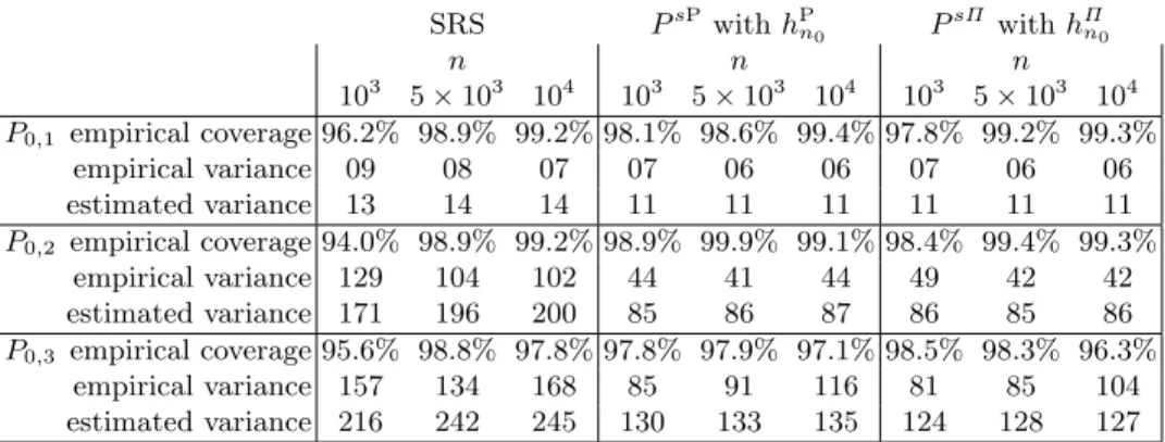
The results are summarized in Table 0.1. We focus on the empirical coverage, empirical variance and mean of the estimated variance of the TMLE.
SRS PsP withhPn0 P sΠ withhΠn0 n n n 103 5×10³ 104 103 5×10³ 104 103 5×10³ 104 P0,1 empirical coverage 96.2% 98.9% 99.2% 98.1% 98.6% 99.4% 97.8% 99.2% 99.3% empirical variance 09 08 07 07 06 06 07 06 06 estimated variance 13 14 14 11 11 11 11 11 11 P0,2 empirical coverage 94.0% 98.9% 99.2% 98.9% 99.9% 99.1% 98.4% 99.4% 99.3% empirical variance 129 104 102 44 41 44 49 42 42 estimated variance 171 196 200 85 86 87 86 85 86 P0,3 empirical coverage 95.6% 98.8% 97.8% 97.8% 97.9% 97.1% 98.5% 98.3% 96.3% empirical variance 157 134 168 85 91 116 81 85 104 estimated variance 216 242 245 130 133 135 124 128 127
Table 0.1.Summarizing the results of the simulation study. The top, middle and bottom groups of rows correspond to simulations underP0,1,P0,2andP0,3. Each of them reports the empirical coverage of the CIs (B−1PBb=11{Ψc(P0,j)∈
In,b}),ntimes the empirical variance of the estimators (n[B−1PB b=1ψ ∗2 n,b−(B −1PB b=1ψ ∗ n,b) 2
]) and empirical mean ofntimes the estimated variance of the estimators (B−1PB
b=1ˆσ 2
n,b), for every sub-sample sizenand for each survey sampling design.
All empirical coverages are larger than 95% but one (equal to 94%). In each case, the mean of estimated variances is larger than the corresponding empirical variance, revealing that we achieve the conservative estimation of σ2
1. Regarding the variances, we observe that PsP and PsΠ perform similarly and provide slightly better results than SRS under P0,1. This is in line with what was expected, due to the contrast induced by the conditional standard deviation of Y given (A, W) under P0,1. Under P0,2, we observe that
PsP andPsΠ perform similarly and provide significantly better results than SRS. This too is in line with what was expected, due to the contrast induced by the conditional standard deviation of Y given (A, W), which is stronger underP0,2than underP0,1. Finally, underP0,3, we observe thatPsPperforms better than SRS and thatPsΠ performs even slightly better than PsP. This again is in line with what was expected, due to the contrast induced by the conditional standard deviation of Y given (A, W) (same as underP0,2) and to the different conditional means ofY given (A, W) underP0,3 andP0,2.
Acknowledgements.
The authors acknowledge the support of the French Agence Nationale de la Recherche (ANR), under grant ANR-13-BS01-0005 (project SPADRO).
7 Elements of proof
For every f ∈ F, let ¯f, f2 be given by ¯f(V)≡E
P0[f(O)|V], f 2(V)≡E P0 f2(O)|V. Note thatf2(V)− ¯ f2(V) = Var P0[f(O)|V].
For every 1≤v≤ν, let `1, . . . , `ν andI1, . . . , Iν be given by`v(V)≡1{V =v} andIv ≡ {1≤i≤N :
Vi=v}.
7.1 Proof of Proposition0.1
Combining (0.3) andA3yields that (1−γn) √ n(ψn∗−ψ0) = √ n(PnHT−P0)D(Pn∗) +oP(1) =√n(PnHT−P0)f1+ √ n(PnHT−P0)(D(Pn∗)−f1) +oP(1),
wheref1∈ F is introduced inA2. ByA1, the first RHS term in the above equation converges in distribution to the centered Gaussian distribution with variance σ21. Moreover, by a classical argument of empirical processes theory (van der Vaart,1998, Lemma 19.24),A1and the convergence ofD(P∗
n) tof1in A2imply that the second RHS term converges to 0 in probability. This completes the sketch of proof.
7.2 Proof of Eq. (0.8) and (0.9)
By construction ofPsΠ, the number of observations sampled from eachV-stratum is deterministic. In other words, it holds for each 1≤v≤ν that VarPsΠ
PnHT`v
= 0. In light of (0.2), this is equivalent to
X i∈Iv 1 Πii −1 = X i6=j∈Iv |Πij|2 ΠiiΠjj (0.15) for each 1≤v≤ν.
Now, sinceVi6=Vj impliesΠij = 0 by construction, (0.2) rewrites
N2VarPsΠ PnHTf = N X i=1 1 Πii −1 f2(Oi)− X 1≤i6=j≤N |Πij|2 f(Oi) Πii f(Oj) Πjj = ν X v=1 X i∈Iv 1 Πii −1 f2(Oi)− ν X v=1 X i6=j∈Iv |Πij|2 ΠiiΠjj f(Oi)f(Oj).
BecauseO1, . . . , ON are conditionally independent given (V1, . . . , VN) and since each factor|Πij|2/ΠiiΠjj is deterministic giveni, j∈Iv, the previous equality and (0.15) then imply
N2EP0 VarPsΠPnHTf= EP0 ν X v=1 f2(v)X i∈Iv 1 Πii −1 − ν X v=1 ¯ f2(v) X i6=j∈Iv |Πij|2 ΠiiΠjj = ν X v=1 f2(v)−f¯2(v)E P0 " X i∈Iv 1 Πii −1 # . (0.16) For each 1≤v≤ν, EP0 " X i∈Iv 1 Πii −1 # = N nh(v)−1 EP0[card(Iv)] = N nh(v)−1 N P0(V =v). Therefore, (0.16) yields
EP0 VarPsΠPnHTf= 1 n ν X v=1 f2(v)−f¯2(v)h−1(v)P 0(V =v)− 1 N ν X v=1 f2(v)−f¯2(v)P 0(V =v) = 1 nEP0 VarP0[f(O)|V]h −1(V) − 1 NEP0[VarP0[f(O)|V]], as stated in (0.8).
We now turn to (0.9). Since EPsΠ PnHTf=PNf, it holds that VarP0PsΠ √ n(PnHT−P0)f=nEP0 EPsΠ(PnHTf)2−n EP0PsΠPnHTf 2 =nEP0 VarPsΠ PnHTf +nVarP0[PNf] =nΣhΠ(f, f) + n N VarP0[f(O)]−EP0[VarP0[f(O)|V]] ,
where the last equality follows from (0.8). This completes the proof.
7.3 Proof of Proposition0.3
Let us first state the so called Soshnikov conditions (Soshnikov, 2000). A function f ofO drawn from P0 meets them if N2VarPsK PnHTf goes to infinity, (0.17) max 1≤i≤NK −1 ii f(Oi) =o N2VarPsKPnHTf for all >0, (0.18) NEPsKPnHT|f|=O N2VarPsKPnHTf δ for some δ >0. (0.19) Conditions (0.17), (0.18) and (0.19) are expressed conditionally on a trajectory (Oi)i≥1 of mutually inde-pendent random variables drawn fromP0. We denote Ω(f) the set of trajectories for which they are met. By assumption, P0(Ω(f)) = 1 for allf ∈ F0. It is worth emphasizing that this assumption may implicitly require that the ration/N go to zero sufficiently slowly, as evident in the sketch of proof of Proposition0.4. SinceF0 is countable,Ω≡ ∩f
∈F0Ω(f) also satisfiesP0(Ω) = 1.
Set f ∈ F0 and define Z
N(f) ≡ (VarPsPnHTf)−1/2(PnHT−P0)f. On Ω, the characteristic function
t 7→ EPsKeitZN(f) converges pointwise to t 7→ e−t
2/2
. Therefore, t 7→ EP0
EPsKeitZN(f)1{Ω} also
does. Since P0(Ω) = 1, this implies the convergence in distribution of ZN(f) to the standard normal law hence, by Slutsky’s lemma, that of √n(PHT
n −P0)f to the centered Gaussian law with a variance equal to the limit in probability of nVarPsKPnHTf. The asymptotic tightness of
√
n(PHT
n −P0)f follows. Finally, applying the Cram´er-Wold device yields the convergence to a centered multivariate Gaussian law of all marginals√n(PnHT−P0)(f1, . . . , fM) withf1, . . . , fM ∈ F0.
The second step of the proof hinges on the following concentration inequality (Pemantle and Peres,2014, Theorem 3.1): ifC(f)≡max1≤i≤N|Kii−1f(Oi)| then, for allt >0,
PsK|(PnHT−P0)f| ≥t
≤2 exp −nt2/8C(f)2. (0.20) This statement is conditional onO1, . . . , ON. Note that there exists a deterministic upper-bound to allC(f)s becauseF0 is uniformly bounded and because the first order inclusion probabilities are bounded away from 0 uniformly in N. We go from the convergence of all marginals toA1 by developing a so called chaining argument typical of empirical processes theory. The argument builds upon (0.20) and the assumed finiteness of the bracketing entropy ofF0 with respect to the supremum norm. This completes the sketch of the proof.
7.4 Proof of Proposition0.4
PnHTf = 1 n ν X v=1 f(v)h−1(v)nv, where nv =P N i=1ηi`v(Vi) = nh(v)Nv/N with Nv ≡ P N
i=1`v(Vi) (each 1≤ v ≤ ν). Therefore, the above display rewritesPHT
n f =PNf, hence VarPsΠPnHTf= 0. Moreover, the CLT for bounded, independent and
identically distributed observations implies √n(PHT
n −P0)f = p n/N×√N(PN −P0)f =OP( p n/N) = oP(1) .
Consider nowf ∈ F0. We wish to prove thatf meets the Soshnikov conditions and thatnVar
PsΠPnHTf
converges inP0-probability to ΣhΠ(f, f), which is positive becausef ∈ F0. When relying onP
sΠ, the LHS expression in (0.18) rewrites max1≤i≤NN f(Oi)/nh(Vi) and is clearly upper-bounded by a constant times
N/n. As for the LHS of (0.19), it equals PN
i=1|f(Oi)| and is thus clearly upper-bounded by a constant times N. Let us now turn to VarPsΠPnHTf. By construction of PsΠ, the variance decomposes as the
sum of the variances over eachV-stratum, each of them being a quadratic form in sub-Gaussian, indepen-dent and iindepen-dentically distributed random variables conditionally on (V1, . . . , VN). Because quadratic forms of independent sub-Gaussian random variables are known to concentrate exponentially fast around their expec-tations (see the Hanson-Wright concentration inequality inRudelson and Vershynin,2013), VarPsΠ
PnHTf
concentrates around its expectation (0.8). Consequently,N2Var
PsΠPnHTfis of orderN2/n. It is then clear
thatN/n=o((N2/n)) for all >0 ensures that f meets the Soshnikov conditions. This holds for instance ifn≡N/loga(N) for some a >0. Finally, the concentration of VarPsPnHTfaround its expectation also
yields the convergence ofnVarPsPnHTfto ΣhΠ(f, f) inP0-probability.
At this point, we have shown that √n(PHT
n −P0)f converges in distribution to the centered Gaussian law with varianceΣΠ
h(f, f). The rest of the proof is similar to the end of the proof of Proposition0.3. This completes the sketch of proof.
References
P. Bertail, A. Chambaz, and E. Joly. Practical targeted learning from large data sets by survey sampling.
arXiv preprint, 2016a. Submitted.
P. Bertail, E. Chautru, and S. Cl´emen¸con. Empirical processes in survey sampling. Scandinavian Journal of Statistics, 2016b. To appear.
L. Bondesson, I. Traat, and A. Lundqvist. Pareto sampling versus Sampford and conditional Poisson sam-pling. Scandinavian Journal of Statistics. Theory and Applications, 33(4):699–720, 2006.
A. Chambaz and P. Neuvial. Targeted, integrative search of associations between DNA copy number and gene expression, accounting for DNA methylation. Bioinformatics, 31(18):3054–3056, 2015.
A. Chambaz and P. Neuvial. Targeted Learning of a Non-Parametric Variable Importance Measure of a Continuous Exposure, 2016. URLhttp://CRAN.R-project.org/package=tmle.npvi. R package version 0.10.0.
A. Chambaz, P. Neuvial, and M. J. van der Laan. Estimation of a non-parametric variable importance measure of a continuous exposure. Electron. J. Stat., 6:1059–1099, 2012.
J. Hajek. Asymptotic theory of rejective sampling with varying probabilities from a finite population. The Annals of Mathematical Statistics, 35(4):1491–1523, 12 1964.
M. Hanif and K. R. W. Brewer. Sampling with unequal probabilities without replacement: a review. Inter-national Statistical Review/Revue InterInter-nationale de Statistique, pages 317–335, 1980.
J. B. Hough, M. Krishnapur, Y. Peres, and B. Vir´ag. Determinantal processes and independence. Probability Surveys, 3:206–229, 2006.
V. Loonis and X. Mary. Determinantal sampling designs.arXiv preprint arXiv:1510.06618, 2015. Submitted. R. Lyons. Determinantal probability measures. Publications Math´ematiques de l’Institut des Hautes ´Etudes
Scientifiques, 98:167–212, 2003.
O. Macchi. The coincidence approach to stochastic point processes. Advances in Applied Probability, 7: 83–122, 1975.
R. Pemantle and Y. Peres. Concentration of Lipschitz functionals of determinantal and other strong Rayleigh measures. Combinatorics, Probability and Computing, 23(1):140–160, 2014.
M. Rudelson and R. Vershynin. Hanson-Wright inequality and subgaussian concentration. Electron. Com-mun. Probab., 18(82):1–9, 2013.
M. R. Sampford. On sampling without replacement with unequal probabilities of selection. Biometrika, 54 (3-4):499–513, 1967.
A. Soshnikov. Gaussian limit for determinantal random point fields. Ann. Probab., 30(1):171–187, 2000. M. J. van der Laan. One-step targeted minimum loss-based estimation based on universal least favorable
one-dimensional submodels. International Journal of Biostatistics, 2016. To appear.
M. J. van der Laan and S. Lendle. Online targeted learning. Technical Report 330, Division of Biostatistics, University of California, Berkeley, 2014.
A. W. van der Vaart. Asymptotic statistics, volume 3 ofCambridge Series in Statistical and Probabilistic Mathematics. Cambridge University Press, Cambridge, 1998.
A. W. van der Vaart and J. A. Wellner. Weak Convergence and Empirical Processes. Springer, Berlin Heidelberg New York, 1996.