An Analysis of Claim Frequency and Claim Severity for Third
Party Motor Insurance Using Monte Carlo Simulation
Techniques
by
Cedric Dumais
A thesis submitted in partial fulfilment
of the requirements for the degree of
Master of Science (MSc) in Computational Sciences
The Faculty of Graduate Studies
Laurentian University
Sudbury, Ontario, Canada
ii
THESIS DEFENCE COMMITTEE/COMITÉ DE SOUTENANCE DE THÈSE Laurentian Université/Université Laurentienne
Faculty of Graduate Studies/Faculté des études supérieures
Title of Thesis
Titre de la thèse An Analysis of Claim Frequency and Claim Severity for Third Party Motor Insurance Using Monte Carlo Simulation Techniques
Name of Candidate
Nom du candidat Dumais, Cedric
Degree
Diplôme Master of Science
Department/Program Date of Defence
Département/Programme Computational Sciences Date de la soutenance August 22, 2019
APPROVED/APPROUVÉ Thesis Examiners/Examinateurs de thèse:
Dr. Peter Adamic
(Supervisor/Directeur(trice) de thèse) Dr. Youssou Gningue
(Committee member/Membre du comité) Dr. Hafida Boudjellaba
(Committee member/Membre du comité)
Approved for the Faculty of Graduate Studies
Approuvé pour la Faculté des études supérieures
Dr. David Lesbarrères
Monsieur David Lesbarrères
Dr. Franck Adékambi Dean, Faculty of Graduate Studies
(External Examiner/Examinateur externe) Doyen, Faculté des études supérieures
ACCESSIBILITY CLAUSE AND PERMISSION TO USE
I, Cedric Dumais, hereby grant to Laurentian University and/or its agents the non-exclusive license to archive and make accessible my thesis, dissertation, or project report in whole or in part in all forms of media, now or for the duration of my copyright ownership. I retain all other ownership rights to the copyright of the thesis, dissertation or project report. I also reserve the right to use in future works (such as articles or books) all or part of this thesis, dissertation, or project report. I further agree that permission for copying of this thesis in any manner, in whole or in part, for scholarly purposes may be granted by the professor or professors who supervised my thesis work or, in their absence, by the Head of the Department in which my thesis work was done. It is understood that any copying or publication or use of this thesis or parts thereof for financial gain shall not be allowed without my written permission. It is also understood that this copy is being made available in this form by the authority of the copyright owner solely for the purpose of private study and research and may not be copied or reproduced except as permitted by the copyright laws without written authority from the copyright owner.
Abstract
The purpose of this thesis is to introduce the reader to Multiple Regression and Monte Carlo simulation techniques in order to find the expected compensation cost the insurance company needs to pay due to claims made. With a fundamental understanding of prob-ability theory, we can advance to Markov chain theory and Monte Carlo Markov Chains (MCMC). In the insurance field, in particular non-life insurance, expected compensation is very important to calculate the average cost of each claim. Applying Markov models, simulations will be run in order to predict claim frequency and claim severity. A variety of models will be implemented to compute claim frequency. These claim frequency results, along with the claim severity results, will then be used to compute an expected compen-sation for third party auto insurance claims. Multiple models are tested and compared.
Keywords
Regression, MCMC, Gibbs Sampler, Logistic, Poisson, Negative Binomial, Zero-Inflated, Insurance, Claim Frequency, Claim Severity, Expected Compensation
Contents
1 Introduction 1
2 Literature Review 3
2.1 Poisson Model . . . 3
2.1.1 Poisson Regression Model . . . 4
2.2 Negative Binomial Model . . . 8
2.2.1 Negative Binomial Regression Model . . . 9
2.3 Zero-Inflated Poisson Model . . . 10
2.4 Zero-Inflated Negative Binomial Model . . . 12
2.5 Gamma Model . . . 13
2.5.1 Gamma Regression Model . . . 15
2.6 Collective Risk Model . . . 15
2.7 Markov Chain Monte Carlo . . . 17
2.7.1 Gibbs Sampler . . . 19
2.7.2 Heidelberg and Welch Test . . . 24
2.8 Model Comparison . . . 25
3 Data 26 4 Application of Claim Frequency, Severity and Expected Compensation 29 4.1 Claim Frequency . . . 29
4.1.2 Negative Binomial and Zero-Inflated Negative Binomial Models . . . 30 4.2 Claim Severity . . . 31 4.2.1 Gamma Model . . . 31 4.3 Expected Compensation . . . 32 4.4 Residual Analysis . . . 33 4.5 Bayesian Inference . . . 35 4.5.1 Prior Distributions . . . 35 4.5.2 Posterior Distribution . . . 36
4.6 Markov Chain Monte Carlo Application . . . 38
4.6.1 MCMC Calculations . . . 38
5 Results 40 5.1 Claim Frequency . . . 40
5.1.1 Poisson Model . . . 40
5.1.2 Zero-Inflated Poisson Model . . . 50
5.1.3 Negative Binomial Model . . . 56
5.1.4 Zero-Inflated Negative Binomial Model . . . 64
5.1.5 Comparison . . . 70
5.2 Claim Severity . . . 71
5.2.1 Gamma Model . . . 71
5.3 Expected Compensation . . . 78
7 Future Work 83
References 85
Appendix 89
List of Tables
3.1 Summary Statistics for the Third Party Insurance Data . . . 27
4.1 Regression Covariates . . . 31
5.1 Poisson Heidelberg and Welch diagnostics. . . 44
5.2 Poisson Posterior Results . . . 45
5.3 Poisson Credible Intervals . . . 46
5.4 Claim Frequency by Area (Poisson Results) . . . 47
5.5 Zero-Inflated Poisson Heidelberg and Welch diagnostics . . . 53
5.6 Zero-Inflated Poisson Posterior Results . . . 53
5.7 Zero-Inflated Poisson Credible Intervals. . . 54
5.8 Claim frequency by zone (Zero-Inflated Poisson) . . . 55
5.9 Negative Binomial Heidelberg and Welch diagnostics . . . 62
5.10 Negative Binomial Posterior Results . . . 62
5.11 Negative Binomial Credible Intervals . . . 63
5.12 Claim Frequency by Zone (Negative Binomial Results) . . . 63
5.13 Zero-Inflated Negative Binomial Heidelberg and Welch Diagnostics . . 67
5.15 Zero-Inflated Negative Binomial Credible Intervals . . . 68
5.16 Claim Frequency by Zone (Zero-Inflated Negative Binomial Results) . . 69
5.17 DIC Criterion for Claim Frequency . . . 70
5.18 Gamma Heidelberg and Welch Diagnostics . . . 74
5.19 Gamma Posterior Results . . . 75
5.20 Gamma Credible Intervals . . . 75
5.21 Claim Severity by Zone (Gamma Results) . . . 76
5.22 DIC scores for the Gamma Model. . . 76
5.23 Expected Compensation by Zone . . . 81
7.1 95% Credible Interval for Claim Frequency (Poisson Model) . . . 89
7.2 Claim Frequency by Zone and Kilometres Driven per Year (Poisson Model). . . 89
7.4 Claim Frequency by Zone and Kilometres Driven per Year (Zero-Inflated Poisson Model) . . . 92
7.6 Claim Frequency by Zone and Kilometres Driven per Year (Negative Binomial Model) . . . 94
7.3 Credible intervals for claim frequency by zone (Zero-Inflated Poisson) 97 7.5 95% Credible Interval for Negative Binomial Posterior Claim Frequency 98 7.7 95% Credible Interval for Zero-Inflated Negative Binomial Claim Fre-quency . . . 99
7.8 Claim Frequency by Zone and Kilometres Driven per Year (Zero-Inflated Negative Binomial Model) . . . 100 7.9 95% Credible Interval for Claim Severity (Gamma Model). . . 102
List of Figures
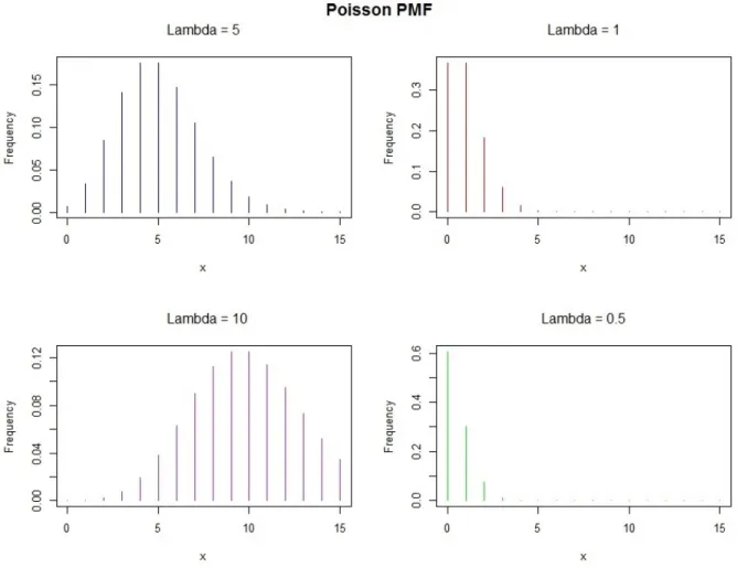
2.1 Probability Mass function for Poisson Distributions . . . 7 2.2 Probability Mass function for Negative Binomial Distributions withµ= 2. 10 2.3 Density function for Gamma Distributions . . . 14 3.1 Density of Claims with a Gaussian Kernel and Bandwidth of 1.922. . . 28 5.1 Trace Plots and Posterior Density Plots for Poisson Iterations. 3 Chains
With 30,000 Iterations Each . . . 42 5.2 Autocorrelation Plot for Poisson Iterations . . . 43 5.3 Residual Plot for Poisson Model . . . 49 5.4 Trace Plots and Posterior Density Plots for Zero-Inflated Poisson
Iter-ations. 3 Chains With 300,000 Iterations Each . . . 51 5.5 Autocorrelation Plot for Zero-Inflated Poisson Iterations . . . 52 5.6 Residual Plot for Zero-Inflated Poisson Model . . . 56 5.7 Trace Plots and Posterior Density Plots for Negative Binomial
Itera-tions. 3 Chains With 75,000 Iterations Each. . . 58 5.8 Autocorrelation Plot for Negative Binomial Iterations . . . 59 5.9 Residual Plot for Negative Binomial Model . . . 61
5.10 Trace Plots and Posterior Density Plots for Zero-Inflated Negative Bi-nomial Iterations. 3 Chains With 400,000 Iterations Each . . . 65 5.11 Autocorrelation Plot for Zero-Inflated Negative Binomial Iterations. . . 66 5.12 Residual Plot for Zero-Inflated Negative Binomial Model . . . 69 5.13 Trace Plots and Posterior Density Plots for Gamma Iterations. 3 Chains
With 75,000 Iterations Each . . . 72 5.14 Autocorrelation Plot for Gamma Iterations . . . 73 5.15 Residual Plot for Gamma Model (1e3) . . . 77
1
Introduction
In today’s society, we place a high importance on modelling and predicting various types of risks. This allows for protection against various financial insecurities that might otherwise cause significant harm to our financial security. Such risks we model include non-life insurance or property and casualty insurance. In the field of personal casualty insurance, actuaries are often tasked with modelling auto insurance claims. The goal of the insurance company is to calculate an effective insurance price or premium to the corresponding insured party in order to cover the necessary risk. Claim frequency, also known as count data, and claim severity are the variables used to calculate the average cost of claims for property and casualty insurance. A superior model for claim frequency and claim severity means more competitive fees and in turn, a more profitable coverage for the insurer. Therefore, modelling claim frequency and claim severity is a crucial step for pricing personal and casualty insurance.
In the past, there has been extensive interest in count data models, particularly in Actu-arial Science. Generalized linear models (GLMs) were given a life of their own by [Nelder and Wedderburn, 1972]. The use of generalized linear models by statisticians and ac-tuaries has been discussed by [Haberman and Renshaw, 1996] as well as [Renshaw, 1994] and [McCullagh and Nelder, 1989]. Although these GLM models do many things well, they have several disadvantages. The assumptions made by GLM’s may not hold true and therefore, the predictiveness of the model can be suboptimal. Residuals of the GLM’s in insurance data are rarely homogeneous; an important feature in scoring a
mod-els fit. Lastly, GLM’s only offer correlation between variables rather than causation. As shown in [Panjer and Willmot, 1983], the statistical interpretation of risk is essentially Bayesian. The approach adopted here is fully Bayesian, allowing for causation, model flexibility and credible intervals. To actuate this Bayesian approach, Markov Chain Monte Carlo (MCMC) is used for parameter estimation.
In this thesis statistical models for the claim frequency in Third Party Motor insurance are compared. Poisson regression has been the primary regression to model claim fre-quencies in the past. As has been shown in [Gourieroux and Jasiak, 2001], the Poisson distribution has many limitations due to its equidispersion. Equidispersion is defined as the equality of mean and variance within a distribution. To give an alternative, the Poisson regression model is compared with the Negative Binomial regression. Subsequently, the Zero-inflated models are compared as well. The claim severity is modeled by a Gamma model. In order to predict the expected compensation, the expected claim frequency is multiplied by the expected claim severity. The MCMC with Gibbs sampling will be used for parameter estimation. The models will then be scored by fit, and compared using the Deviance Information Criterion (DIC). A comparison of cost savings when using the best fitted model is given. Based on these models, the total claim severity can be simulated for premium calculation. The dependencies between the number of claims and claim severity is allowed. This regression takes into consideration the Poisson distribution as well as the Negative Binomial distribution to model the claim frequency and the Gamma distribution
to model the claim severity.
The contributions of this thesis are to provide four models to quantify and estimate claim frequency. Provide a Gamma model to estimate claim severity. Compute the expected compensation for the different zones of policyholders. Discuss strengths and weaknesses of each count variable model obtained by MCMC. Discuss and provide an example of regression model comparison with a Bayesian approach for auto claim frequencies.
2
Literature Review
In this chapter the review of the literature employed in the thesis is explained. An intro-duction to Poisson regression, Negative Binomial regression and Gamma regression is given. Markov Chain Monte Carlo (MCMC) and Gibbs sampling is reviewed, along with the Deviance Information Criterion used to compare the models.
2.1
Poisson Model
To begin, the Poisson distribution is introduced. The benchmark model for count data is the Poisson distribution. It is useful at the outset to review some fundamental properties and characterization results. If the discrete random variableY is Poisson-distributed with intensity or rate parameterµ, µ > 0, andt is the exposure, defined as the length of time
during which the events are recorded, thenY has density of the Poisson distribution
P r[Y =y] = e
−µt(µt)y
y! , y= 0,1,2... (1)
whereE[Y] =V[Y] =µt. If the length of the exposure periodtis equal to unity, then
P r[Y =y] = e
−µµy
y! , y = 0,1,2, ... (2)
This distribution has a single parameterµ, and is referred to asP[µ]. Its kth raw moment,
E[Yk], may be derived by differentiating the moment generating function k times. The
Poisson distribution has equal mean and variance. This is referred as equidispersion. This property is often violated in real-life data. Overdispersion (underdispersion) means the variance exceeds (is less than) the mean.
The law of rare events states that the total number of events will follow, approximately, the Poisson distribution if an event may occur in any of a large number of trials but the probability of occurrence in any given trial is small. More formally, letYn,π denote the total
number of successes in a large number n of independent Bernoulli trials with success probabilityπof each trial being small. Then
P r[Yn,π =k] = n k πk(1−π)n−k, k= 0,1, ..., n. (3)
2.1.1 Poisson Regression Model
A standard application of Poisson regression is to cross-section data [Cameron and Trivedi, 2013]. Typical cross-section data for applied work consist of n independent ob-servations, theithof which is(yi, xi). The scalar dependent variable,yi, is the number of
occurrences of the event of interest, andxiis the vector of linearly independent regressors
that are thought to determineyi . A regression model based on this distribution follows by
conditioning the distribution ofyion a k-dimensional vector of covariates,xi = [x1i, ..., xki],
and parameters β, through a continuous function µ(xi, β), such that E[yi|xi] = µ(xi, β).
That is,yi given xi is Poisson-distributed with probability density
f(yi|xi) =
e−µiµyi
i
yi!
, yi = 0,1,2, . . . (4)
In the log-linear version of the model, the mean parameter is parameterized as
µi =exp(x0iβ), (5)
to ensure µ > 0. These two equations jointly define the Poisson (log-linear) regression model. For notational economy f(yi|xi) is written in place of the more formal f(Yi =
yi|xi), which distinguishes between the random variable Y and its realization y. By the
property of the Poisson, V[yi|xi] = E[yi|xi], implying that the conditional variance is not
a constant, and hence the regression is intrinsically heteroskedastic. This is to say that the variance of the residual terms varies widely. In the log-linear version of the model the mean parameter is parameterized as Equation (5), which implies that the conditional mean has a multiplicative form given by
E(yi|xi) = exp(x0iβ)
=exp(x1iβ0)exp(x2iβ1)· · ·exp(xkiβk),
(6)
with interest often lying in changes in this conditional mean due to changes in the regres-sors. The additive specification,E[yi|xi] = x0iβ =
Pk
because certain combinations ofβi and xi will violate the nonnegativity restriction on µi.
In most cases, x1 = 1, β0 is interpreted as the intercept, and β1, . . . , βk are unknown
parameters. For example, let y be the observed number of accidents, N be the known exposure risk, and x the known explanatory variables. The mean number of events µis expressed as the product ofN andti. This is often called the rate of occurrence. That is,
µ(x) = N(x)ti(x, β). The expected value for this rate of occurrence with exposure variable
ti is
E(yi|xi) =tiλ(x0iβ)
=tiexp(β0+β1X1i+. . .+βkXki).
(7)
Therefore, for a given set of regressor variables, the outcome (dependent variable) follows a Poisson Distribution.
2.2
Negative Binomial Model
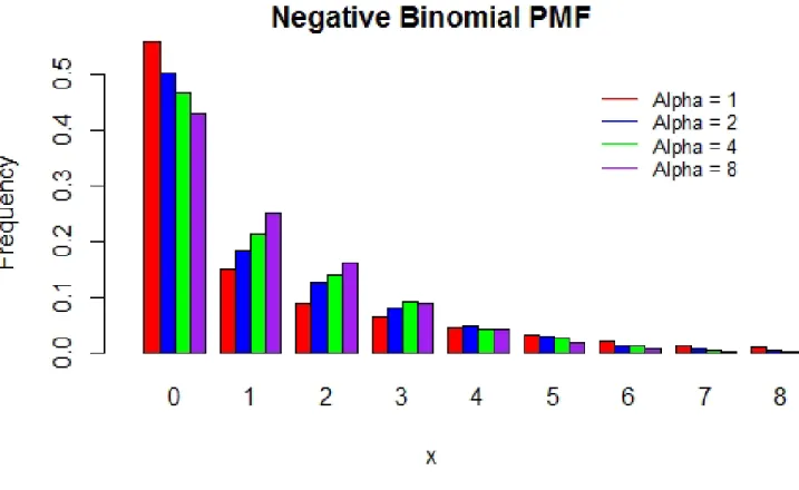
In this thesis the commonly known NB2 model introduced by [Cameron and Trivedi, 1986] is used. The most common way this model is derived is by assuming the data are Poisson, but there is gamma-distributed unobserved individual heterogeneity reflecting the fact that the true mean is not perfectly observed. This model has a scale parameter ofα= v1.
P r(Y =yi|µi, α) = Γ(yi+α−1) Γ(yi+ 1)Γ(α−1) α−1 α−1+µ i α−1 µi α−1+µ i yi , (8) where µi =tiµ α= 1 v.
The parameterµis the mean ofyper unit of exposureti. The mean is calculated by
E(yi) =µi =ex
t
iβ, (9)
and the variance by
V ar(yi) = σi2 =µi(1 +αµi). (10)
It is shown below that in Equation (8) when α → 0, the Poisson distribution is obtained. This is because α is known as the dispersion parameter. α−1 is referred to as the index
or dispersion parameter. From [Cameron and Trivedi, 2013], f(y) = y=1 Y j=0 (j +α) 1 y! α α+µ α 1 α+µ y µy = y=1 Y j=0 j +α α+µ α α+µ α µy 1 y! = y=1 Y j=0 1 + αj 1 + µα 1 1 + µα α µy 1 y! →1e−µµy 1 y! as α→ ∞. Since 1e−µµy 1
y! is the Poisson distribution, the Poisson is the special case as α → 0. As
with the Poisson distribution, the parameterµis the incidence rate per unit of exposureti.
The functionΓ(·)is the gamma function and defined by
Γ(α) =
Z ∞
0
e−ttα−1dt, α >0. (11)
Therefore, the Negative Binomial distribution given by Equation (8) is represented as a Poisson-Gamma mixture distribution.
2.2.1 Negative Binomial Regression Model
The Negative Binomial regression model is determined by exposure time tandk regres-sor variables. The expected value is expressed as
µi =exp(ln(ti) +β0+β1x1i+. . .+βkxki). (12)
In Negative Binomial regression, whereµis the mean andβ0 is the intercept. The
Figure 2.2: Probability Mass function for Negative Binomial Distributions withµ= 2.
set. Therefore, a Negative Binomial regression model for an observationiis given as
P r(Y =y|µi, α) = Γ(yi+α−1) Γ(α−1)Γ(y i+ 1) 1 1 +αµi α−1 αµi 1 +αµi yi , (13)
whereyis the dependent variable.
2.3
Zero-Inflated Poisson Model
The zero-inflated Poisson model was introduced by [Lambert, 1992] to solve problems with the large zero counts in data. The zero-inflated models are a solution to incorrect
and biased models, incorrect parameter estimations, biased errors and over-dispersion caused by the high zero counts in the dataset. The zero-inflated Poisson is a two part model, consisting of both binary and count model sections. Suppose that for each obser-vation i, there are two possible cases. If case one occurs, the count is zero. If case two occurs, counts(including zeros) are generated according to the Poisson model. Given the probability of case one to beπ, and the probability of case two to be1−π, the probability distribution of the Poisson is
P r(yi = 0) =πi+ (1−πi)e−µi P r(yi >0) = (1−πi) µyii exp(−µi) yi! , (14) and, V ar(yi) = (1−πi)(µi+µ2i) > µi(1−πi) = E(yi).
The zero-inflated Poisson can be written as
µi =exp(ln(ti) +β0+β1x1i+. . .+βkxki),
where ti is the exposure variable and βi are the regressor variables. The regressor
co-efficients can then be estimated using maximum likelihood estimation or in this case, Bayesian estimation. The goal is to estimate(β, γ). [Lambert, 1992] introduced the model in which µi = µ(xi, β) and the probabilityπi is parameterized as a logistic function of the
observable vector of covariateszi. The logistic link function is given as follows: yi = 0, with probability πi yi ∼P(µi), with probability (1−πi) πi = exp(zi0γ) 1 +exp(zi0γ), (15) where exp(z0iγ) =exp(ln(ti) +γ1z1i+γ2z2i+. . .+γmzmi). (16)
2.4
Zero-Inflated Negative Binomial Model
The zero-inflated Negative Binomial (ZINB) regression model is similar to the Poisson zero-inflated model. A zero-inflated Negative Binomial model will enable us to distinguish between the effect of the splitting mechanism and the over-dispersion induced by indi-vidual heterogeneity [Greene, 1994]. Suppose that for each observation i, there are two possible cases. If case one occurs, the count is zero. If case two occurs, counts(including zeros) are generated according to the Negative Binomial model. Given the probability of case one to beπ, and the probability of case two to be1−π, the probability distribution of the ZINB is
P r(yi = 0) =πi+ (1−πi)g(yi = 0) ifi= 0
P r(yi =k) = (1−πi)g(yi) ifi >0,
(17)
whereπi is the logistic link function defined by
The zero-inflated Negative Binomial model can also be expressed as
µi =exp(ln(ti) +β0+β1x1i+. . .+βkxki)
whereti is the exposure variable andβi are the regressor variables. The regressor
coef-ficients are then estimated using Bayesian estimation.
2.5
Gamma Model
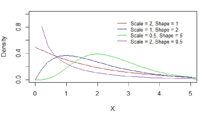
The Gamma distribution is a two-parameter family of continuous probability distributions. It has parameter β and shape parameter α, α > 0 and β > 0. As shown in [Gelman et al., 2013], the Gamma distribution is the conjugate prior distribution for the inverse of the normal variance and for the mean parameter of the Poisson distribution. Let θ be a random variable and θ ∼ Gamma(α, β); that is, the random variable θ follows a Gamma distribution with parametersα andβ. The density function of a Gamma distribution given by the random variableθ is
f(θ;β, α) = β
Γ(α)(βθ)
α−1
e−βθI(0,∞)(θ), (19)
whereI(.)is an indicator function. Under this parameterization, the mean is given by
E(θ) = α
β, (20)
and the variance by
V ar(θ) = α β2 = µ 2 α. (21)
Figure 2.3: Density function for Gamma Distributions
By settingβ = αµ, it is shown in [Gelfand et al., 2005] that the Gamma density function can be written as f(θ) = 1 θΓ(α) αθ µ α exp αθ µ I(0,∞)(θ). (22)
2.5.1 Gamma Regression Model
LetYi ∼G(µi, α)for i = 1,2, . . . , n, be independent random variables. Then the Gamma
regression model is defined as
g(µi) =x0iη
µi =η0x0i+η1x1i+. . .+ηkxki,
(23)
where η = (η0, η1, . . . , ηp)0 is a vector of unknown regression parameters (p < n), xi =
(xi1, xi2, . . . , xip)0 is the vector of p covariates and ηi is a linear predictor. As in most
regression models,x01= 1 for alliso that the model has interceptη0.
2.6
Collective Risk Model
In the basic insurance risk model from [Embrechts et al., 2013], the number of claims and the total claim produced in a given time periodt = 1,2, . . . , T for some classiis denoted by(Nit, Xit)where Xit = PNit k=1 Witk Nit >0 0 otherwise, (24)
and whereWitkis the amount of thekthclaim at timetfor some classi. The assumptions
for the model are given in [Migon and Moura, 2005], and they are:
• The number of claims in the interval(t−1, t]is a random variable denoted asNit
• Conditional on Nit = nit, the claim severity Wik, k = 1,2, . . . , nit, are positive
indepen-dent and iindepen-dentically distributed random variables with finite meanµi = E(Wik)and
• The claims occur at random times t1i ≤ t2i ≤ . . . and the inter-arrival times Tji =
tji −tj−1,i are assumed to be independent and identically exponentially distributed
random variables with finite meanE(Tji) = λ−i 1.
By assuming the sequences Tj and Wj are mutually independent from each other and
identically distributed, the above conditions hold. It follows that Nit is a homogeneous
Poisson process with rate λit, then
Pπit
k=1Nitk|λit ∼ P oisson(λitπit), ηit is the observed
number of claims at time t, for class i and πit is the insured population at time t for
class i, and not πt, t. Assuming that Witk ∼ Gamma(αit, θit), the inter-arrival times are
exponentially distributed. The Poisson-Gamma model is given by
Nit|λit, πit ∼P oisson(λitπit), λi >0
Witk ∼Gamma(αit, θit),
Xit|ηit, θit ∼Gamma(ηitαit, θit) θi >0
(25)
whereαit =ηitαi, ηit is the observed number of claims at timet, for classi andπit is the
insured population at timet for classi.
A similar idea is applied to the Negative Binomial expected values and the Gamma ex-pected values. [Kaas et al., 2008]S =X1, X2, . . . , XN andXiare amounts for a claim and
N is the total amount of claims andS is the sum of the collective claims. The expected value is given by
and the variance
V ar(S) = E(N)V ar(X) + (E(X))2V ar(N). (27) Therefore, the premium for collective risk is given by
P =E(N)E(X). (28)
2.7
Markov Chain Monte Carlo
MCMC is essentially Monte Carlo integration using Markov chains. Scientists need to integrate over possibly high-dimensional probability distributions to make inference about model parameters or to make predictions. Markov Chain Monte Carlo (MCMC) algorithms have made a significant impact on problems where Bayesian analyses can be applied; see [Spiegelhalter et al., 1996]. MCMC can be broken down into key steps, first, randomly generating numbers also known as the Monte Carlo part. Second, allow the numbers generated to influence the next number, also known as the Markov chain part. Third, check for convergence to a reasonable distribution. Monte Carlo integration evaluates
E[f(x)]by drawing samplesXt, t = 1, . . . , nfromπ(.)and then approximating
E[f(X)]≈ 1 n n X t=1 f(Xt). (29)
So the population mean of f(X)is estimated by a sample mean. When the samples Xt
are independent, the law of large numbers ensures that the approximation can be made as accurate as desired by increasing the sample size n. In general, drawing samples Xt
independently fromπ(.)is not feasible sinceπ(.)can be non-standard full conditional dis-tributions. However,Xtdoes not necessarily need to be independent. It can be generated
by any process which draws samples throughout support ofπ(.). SupposeX0, Xl, X2, . . .
are generated as a sequence of random variables, such that at each timet ∼0, the next state Xt+l is sampled from a distribution P(Xt+1|Xt) which depends only on the current
state of the chain,Xt. That is, givenXt, the next stateXt+1does not depend further on the
history of the chain (X0, X1, . . . , Xt−1). This sequence is called a Markov chain. In
gen-eral, MCMC involves simulating from a complex and multivariate target distribution,p(X), by generating a Markov chain with the target density as its stationary density, [Gelman et al., 2013]. Markov chain simulation is used when it is not possible or not computation-ally feasible to sample X directly from p(X|y). Instead, the method draws iteratively in such a way that at each step, the draw from the distribution is expected to be closer to
p(X|y). The basic principle is that once the chain has run sufficiently long enough, it will approximate the posterior distributionp(X|y). In general, m≥ 1independent sequences of simulations are run, each with a length ofn,(Xj1, Xj2, . . . , Xjn)forj = 1, . . . , m.
The term Markov chain stands for a sequence of random variables X1, X2, . . . for which,
for anyt, the distributionXt depends only on the most recent variable,Xt−1. To begin an
MCMC simulation is made by selecting aX0and then for eacht,Xtis drawn from a
transi-tion distributransi-tionTt(Xt|Xt−1)so that the Markov chain hopefully converges to the posterior
distributionp(X|y). Once algorithms have been implemented and the simulations drawn, it is extremely important to ensure the convergence of the simulated sequences. The sequence is monitored with a time-series plot, and the Gelman Rubin method is used to
diagnose convergence, [Brooks and Gelman, 1998]. More on how the MCMC is applied is discussed in Section 2.7.1.
The two most prevailing techniques used in MCMC are the Metropolis-Hastings algorithm and the Gibbs sampler. Bayes’ theorem, can be conceptualized as
posterior∝prior×likelihood. (30)
That is, the posterior is proportional to the likelihood times the prior. The guidelines below flow directly from this theorem:
• If the prior is uninformative, the posterior is determined by the data
• If the prior is informative, the posterior is a mixture of the prior and the data
• The more informative the prior, the more data is needed to influence the beliefs since the posterior is determined more so from the prior information
• If the dataset is large, the data will dominate the posterior distribution
2.7.1 Gibbs Sampler
The Gibbs sampler was introduced by [Geman and Geman, 1984]. Although the Metropolis-Hastings is more commonly used in the literature, the Gibbs sampler was implemented in this thesis since the data analysed is low-dimensional. Low-dimensional refers to the features of the dataset or the amount of variables in the model. High-dimensional data may consist of hundreds or thousands of features. Gibbs sampling can be understood as
running a sequence of low-dimensional conditional simulations. It is used when decompo-sition’s into such conditionals are easy to implement and fast to run, which is the case in this thesis. As described in [Gill, 2002], the Gibbs sampler is useful in producing Markov chain values. It is a special case of the Metropolis-Hastings algorithm with a probability of acceptance of one. Suppose a joint densityf(x, y1, . . . , yp)is given and the marginal
den-sityf(x)is needed to calculate the marginal mean or variance. The most natural way to do so would be to integratef(x)directly. However, in some cases, it is simpler to sample from a conditional distribution than to marginalize by integrating over a joint distribution. Gibbs sampling generates a sample X1, . . . , Xn ∼ f(x) without requiring f(x) [Casella
and George, 1992]. By simulating a large enough sample, the mean, variance, or any other characteristic of f(x) can be calculated. As an example, to calculate the mean of
f(x), lim m→∞ Pm i=1Xi m = Z ∞ −∞ xf(x)dx=E[X]. (31)
is used. By taking m large enough in Equation (31), any population characteristic, even the density itself, can be obtained to any degree of accuracy. The basic tenet of Gibbs sampling is that one can express each parameter to be estimated as conditional on all the others. By going through these conditional distributions, eventually the chain converges to the true joint distribution of interest. Suppose k samples are needed of
X = (x1, . . . , xn)from a joint distributionp(x
(i)
1 , . . . , x
(i)
n
. Let theith sample be denoted by
X(i) = x(1i), . . . , x(ni)
sampleX(i+1) is given by
X(i+1) = x(1i+1), x2(i+1), . . . , x(ni+1),
is a vector. Each component of the vector x(ji+1) is sampled from the distribution of that component conditioned on all other components sampled so far. Therefore,
Xji+1 ∼p x(ji+1)|x(1i+1), . . . , xj(i−+1)1 , x(ji+1) , . . . , x(ni)
is the (i+ 1)th component for the variable x
j. Notice that theith components of the j+ 1
variables are used. This is because the(i+ 1)th component has not been calculated yet.
The above steps are repeatedk times. From these steps, the expected value of any vari-able can be approximated by averaging over all the samples. Since the average over all the samples is used to calculate the characteristics of the variable, it is common to ignore a number of the samples at the beginning (often referred to as the burn-in period). The sample approximates the joint distribution of all variables sinceXi+1 approachesp(X)as
i→ ∞.
To help better describe what is going on with the Gibbs sampler, a simple example is explained. Suppose X and Y are two binary random variables with joint distribution
P(X =x, Y =y) =pX,Y(x, y)given by the following table:
X\Y 0 1 0 0.6 0.1 1 0.15 0.15
That is,pX,Y(0,0) = 0.6. The conditional distribution ofX is easily calculated from Bayes
0)/P(Y = 0) = 0.6/0.75 = 0.8. Starting from some value of X, Y and proceeding to iterate the following two steps will achieve Gibbs sampling. Simulate a new value of X
from P(X|Y = y) where y is the current value of Y. Simulate a new value of Y from
P(Y|X =x) wherex is the current value ofX (generated in 1). Running this simulation via computer program, the summary of the first n = 50 iterations are kept. It is found that the proportion of the iterations in which X = x and Y = y is increasingly close to
P(X = x, Y = y) = pX,Y(x, y). This is a result of simulating a Markov chain whose
stationary distribution isP(X =x, Y =y) =pX,Y(x, y).
Once convergence is achieved, the simulated values are sampled from a distribution that asymptotically follows the target posterior distribution. By increasing the length of the chain (increasing n), the sampling variance of the posterior variables is decreased. The mean and standard deviation, as well as, the na¨ıve standard error and time-series stan-dard error are computed. These error values are measures of the computational MCMC error for the estimation of the posterior expected value. The na¨ıve SE is given as
SEn =
r
V ar(X)
C·S ,
where X is the vector of posterior samples, C is the number of chains run and S is the number of iterations run. Similarly, the time-series SE is given as
SEts =
r
V arts(X)
C·S ,
where V arts(X) is the average of the variance of each set of samplesX for each chain
C. In short, the na¨ıve SE disregards autocorrelation where as the time-series SE takes into account the often high auto correlations found in MCMC sampling. The ensuing trace
plots are time-series plots of the sampled values [Toft et al., 2007]. They are the first tool used to assess the convergence of the chain. If the chain has reached convergence, then the time-series should be centered around a constant mean. If multiple chains with different starting points are plotted, then these plots should seem indistinguishable.
A second test for convergence of chains is the autocorrelation of the monitored parame-ters within each chain. High autocorrelations suggest slow mixing of chains and, usually, slow convergence to the posterior distribution [Smith et al., 2007]. Although the model converges eventually, they are significantly less optimal on computing time compared models with low autocorrelations which tend to converge much faster. A common strategy is to thin the chains to reduce sample autocorrelation. A chain can be thinned by keeping everykthsimulated draw from each sequence. Thinning the chain is an option considered
to improve accuracy, however according to [Link and Eaton, 2012], for approximations of simple features of the target distribution (e.g. means, variances and percentiles), thinning is neither necessary nor desirable.
One approach to get an estimate of the severity of the variance is to run several chains and use the between-chains variance inθˆ. Specifically, ifθˆj denotes the estimate for chain
j(1 ≥ j ≥ m) where each the m chains have the same length, then an estimate for the variance is V ar(ˆθ) = 1 n−1 m X j=1 ˆ θj−θˆ∗ 2 where θˆ∗= 1 n m X j=1 ˆ θj. (32)
2.7.2 Heidelberg and Welch Test
A third test for convergence of the MCMC chain is the Heidelberg and Welch test [Hei-delberger and Welch, 1983]. This is a two part test. In the first part, a test statistic on the entire chain is calculated. The null hypothesis is that the chain is from a stationary distribution. If the null hypothesis is rejected, the first10% of the chain is discarded. This step is repeated until the null hypothesis fails to be rejected or 50% of the chain is dis-carded. For the second part, if the chain passes the first part of the diagnosis, it then takes the part of the chain not discarded from the first part to test the second part. The half-width test calculates half the width of the(1−α)%credible interval around the mean. If the ratio of the half width and the mean is lower than some , then the chain passes the test. Otherwise, the chain must be run for more iterations. The test also provides a key p-value statistic for each variable. The null hypothesis for the test is that the Markov chain are from a stationary distribution.The stationary distribution of a Markov Chain with transition matrix P is some vector, X, such thatXP = X. In other words, over the long run, no matter what the starting state was, the proportion of time the chain spends in state
j is approximately Xj for all j. Simple put, the probability to end (converge) a very long
random walk (Markov chain), is independent of where the walk started. A large p-value means we cannot reject the null hypothesis and that the Markov chains do have a sta-tionary distribution. Therefore, large p-value among these tabled results are an indication for convergence and stationary distribution. This is to say, as i → ∞ there is a unique solution.
2.8
Model Comparison
The deviance information criterion (DIC), introduced by [Spiegelhalter et al., 2002], for a probability modelp(y|θ)with observed data y= (y1, . . . , yn)and unknown parametersθis
defined as
DIC =E[D(θ|y)] +pD. (33)
It considers both model fit as well as model complexity. The goodness-of-fit is measured by the posterior mean of the Bayesian devianceD(θ)defined as
D(θ) =−2logp(y|θ) + 2logf(y), (34)
wheref(y)is some fully specified standardizing term. Model complexity is measured by the number of parameterspD defined by
pD =E[D(θ|y)]−D(E[θ|y]). (35)
The DIC criterion has been suggested as a criterion of model fit by [Spiegelhalter et al., 2002]. DIC is just the sum of the posterior mean deviance and the effective number of parameters. The goal is to find a model that will be best for prediction when taking into account the uncertainty inherent in sampling. According to the criterion, as with other information criterion, the model with the smallest DIC is preferred. The DIC does not give belief for a ”true” model, instead, it provides model comparison for short term predictions. Using the MCMC output, both pD and DIC are easily computed by taking
the posterior mean of the devianceE[D(θ|y)]and the estimate of the deviance D(E[θ|y]). Since 2logf(y) is a standardizing term that is a function of data alone, in the application
of this thesis the standardized term 2logf(y)from Equation (34) is set to zero by setting
f(y) = 1.
3
Data
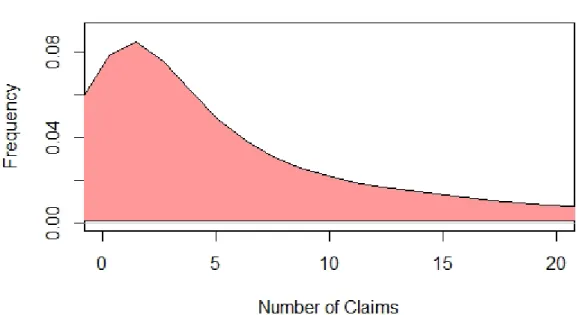
The dataset used in this thesis is a Third Party Motor Insurance dataset from Sweden. In Sweden, all motor insurance companies apply identical risk arguments to classify cus-tomers, and thus their portfolios and their claims statistics can be combined. The data was compiled by the Swedish Committee on the Analysis of Risk Premium in Motor In-surance. This dataset is used to apply the different multiple regressions to compare fits, scores, and show how valuable information can be extracted from the data. The data has a sample size ofn=1937 with 7 variables. The variables are:
• Kilometres: Number of kilometres driven per year
• Zone: Geographical location divided by major cities and surroundings.
• Bonus:No claims made bonus. Equal to the number of years+1 since last claim
• Make of Vehicle: Represents the 8 most driven car models
• Insured: Amount of time insured in policy-years
• ClaimsNumber of Claims made
Table 3.1: Summary Statistics for the Third Party Insurance Data
mean sd median min max
Kilometres 2.985793 1.410409 3.000 1.00 5.0 Zone 3.970211 1.988858 4.000 1.00 7.0 Bonus 4.015124 2.000516 4.000 1.00 7.0 Make 4.991751 2.586943 5.000 1.00 9.0 Insured 1092.195270 5661.156245 81.525 0.01 127687.3 Claims 51.865720 201.710694 5.000 0.00 3338.0 Payment 257007.644821 1017282.585648 27403.500 0.00 18245026.0
The Kilometres driven per year are separated into 5 different categories, <1000, 1000-15000, 15000-20000, 20000-25000, and >25000. The Zones are separated into 7 dif-ferent zones, Stockholm, Goteborg, Malmo with surroundings, Other large cities with sur-roundings, Smaller cities with surroundings in southern Sweden, Rural areas in southern Sweden, Smaller cities with surroundings in northern Sweden, Rural areas in northern Sweden, and Gotland (island). Unfortunately, the make of the cars was never released due to the potential impact on sales. The mean, standard deviation, median, min and max of the data are given below.
The explanatory variables are kilometres driven per year, zone, bonus, make of vehicle, and amount of time insured in policy years. The response variable is the claim frequency.
Figure 3.1: Density of Claims with a Gaussian Kernel and Bandwidth of 1.922.
The payment made is omitted for the claim frequency regressions and is considered later in the claim severity regression. Figure 3.1 depicts the density of claims with bandwidth calculated by what is known as Silverman’s rule of thumb [Silverman, 2018]. The band-width is chosen in order to minimize the mean integrated squared error (MISE). MISE is given asE =R(fn(x)−f(x))2dx, wherefn(x)is the estimate based on sample sizenand
4
Application of Claim Frequency, Severity and Expected
Compensation
As described in Chapter 3, the compound Poisson, the compound Negative Binomial, the zero-inflated Poisson and the zero-inflated Negative Binomial distributions are used to model the claim frequencies. Claim severity follows a Gamma distribution. The claim frequency is modeled by the Poisson, Negative Binomial and the zero-inflated distribu-tions and assumes independence from claim severity. In this Section, all the models are described. The primary result is expected compensation and is obtained by multiplying the expected frequency (from either of the Poisson or Negative Binomial models) by the expected claim severity (from the Gamma model). This is possible because expected compensation assumes independence between claim frequency and claim severity.
4.1
Claim Frequency
For claim frequency, the Poisson model, zero-inflated Poisson model, Negative Binomial model and zero-inflated Negative Binomial model are applied to the dataset. They are scored and compared using residual analysis and the DIC criterion. A fully Bayesian MCMC approach is used to find the posterior distribution of the parameters for both mod-els respectively. Both the Poisson model and Negative Binomial model are tested with different groupings of covariates. The results are compared using the DIC criterion, and subsequently, the best model fits are retained.
4.1.1 Poisson and Zero-Inflated Poisson Models
The first models for claim frequency are the Poisson and Zero-inflated Poisson models. Considering only the observations with non-zero insured policy years, 1937observations are obtained. The following model considers the number of claims Ni, i = 1,2, . . . , n,
observed for each of theith insurance class categories:
Ni|θi ∼P oisson(eit∗θiN), (36)
where
θiN =exp(x0iβ).
Here, eit denotes the insured policy years for policy holder i. The average number of
claims is denoted by θi for class i, xi is a vector of covariates, and β is a vector of
pa-rameters. To estimate the number of claims θi, the vector of unknown parameters is
β = (β0, β1, . . . , β4)0. The vector of covariates for theith policy class observation is given
by xi = (x0i, x1i, . . . , x4i). The matrix obtained from above for the ith observation is
de-scribed in Table 4.1.
4.1.2 Negative Binomial and Zero-Inflated Negative Binomial Models
The second class of model chosen for claim frequency are the Negative Binomial and Zero-inflated Negative Binomial regression models. Just as with the Poisson model, the number of claims observed is Ni, i = 1,2, . . . , n for J insurance class categories. From
Equations (9) and (10),
Ni ∼N egativeBinomial(eit∗θNi , σ
2
Table 4.1: Regression Covariates
Covariate (x) Parameter (β) Description
x0i β0 Intercept
x1i β1 Kilometres
x2i β2 Zone
x3i β3 Bonus
x4i β4 Make
with meanθNi given by
θiN = (exp(x0iβ)),
and variance given as
σi2 =θi(1 +αθi).
The matrix of regression covariates for the Negative Binomial model is the same as that for the Poisson regression covariates given in Table 4.1.
4.2
Claim Severity
4.2.1 Gamma Model
The proposed model for claim severity is the Gamma model. For this model, only ob-servations with a positive number of claims is considered. With this considered, 1797
observations are obtained for the model. The covariance vector is the same as the model for claim frequencyxi = (xi0, xi1, . . . , xi4)0. The vector of unknown regression parameters
is η = (η0, η1, . . . , η4). For policy holders i = 1,2, . . . , n, let Xik, k = 1,2, . . . , Ni, denote
the individual claim severity for theNi observed claims. An individual claim severity
con-ditional onNi is assumed to be independently Gamma distributed:
Xik|Ni ∼Gamma(µSi, v), k= 1,2, . . . , Ni, i= 1,2, . . . , n. (38)
SinceXik|Ni, k = 1,2, . . . , Ni are assumed to be independent and identically distributed,
the average claim severity Xi, given the observed number of claims Ni, is Gamma
dis-tributed with mean and variance
E(Xik|Ni) = µS i v V ar(Xik|Ni) = (µS i)2 v , E Xi = Ni X k=1 Xik Ni |Ni = µ S i v V ar Xi = Ni X k=1 Xik Ni |Ni = (µ S i)2 vNi .
Therefore, the average claim severity for policy holderiis given by
Xi = Ni X k=1 Xik Ni . (39)
4.3
Expected Compensation
One of the primary goals of this thesis is to find the expected compensation cost insurance companies have to pay. As mentioned in Chapter 3, this cost depends on the claim
frequency and claim severity. The expected value of the total cost Xi per number of
years insured ei is a combination of either the Poisson, Zero-inflated Poisson, Negative
Binomial or Zero-inflated Negative Binomial model with the Gamma model. The expected compensation can be expressed as
E Xit eit = 1 eit E(Xit) = 1 eit E Nit X k=1 Witk = 1 eit E(E( Nit X k=1 Witk|Nit)) = 1 eit E(NitE(Wit1)) = 1 eit E(Nit)E(Wit1) = 1 eit E(E(Nit|θitN))µit = 1 eit E(eitθitN)exp(x T iη) =exp(xTi β)exp(xTi η),
where exp(xTi β) is the Poisson or Negative Binomial expected value andexp(xTi η)is the Gamma expected value.
4.4
Residual Analysis
Evaluating model fit has been a controversial subject among Bayesian statistics. Bayesian prior to posterior inferences assume the whole structure of a probability model and can yield misleading inferences when the model is poor. A good Bayesian analysis, therefore,
should include at least some check of the adequacy of the fit of the model to the data and the plausibility of the model for the purposes for which the model will be used [Gelman et al., 2013]. According to [Gelman et al., 2013], it is necessary to examine models by their practical implications as well as tests for outliers, plots of residuals, and normal plots. In this thesis, both practical implications and residual plots are analysed. The practical checks implied are twofold. First, is the model consistent with the data? and second, do the inferences from the model make sense? Residual analysis, in particular graphical analysis, is an important statistical tool used to evaluate the quality of a model fit. Residuals are defined as the difference between the measured output from the data and the predicted model output. When errors in the residuals are not randomly distributed about zero, this suggests the model is not an appropriate fit.
A comprehensive residual analysis is employed. The residuals are plotted against the regressor variables, as well as the response variable to check for any outliers or curvature. Raw residuals are calculated byri =yi−µˆi and analysed. The pearson residual is also
calculated to correct for the unequal variance in the residuals. The Pearson residual is given by pi = yi−µˆi q ˆ φµˆi , where ˆ φ= 1 n−k n X i=1 (yi−µˆi)2 ˆ µi .
For the Negative Binomial regression, the Pearson residual is given as pi = yi−µˆi p ˆ µi+αµˆi2 .
Finally, the hat values are calculated. The hat matrix is used to measure the influence of each observation. The hat values,hii, are the diagonal entries of the hat matrix calculated
using
H =W1/2X(X0W X)−1X0W1/2,
whereW is a diagonal matrix withµˆi. That is, a square matrix withµˆi along the diagonal,
and zeroes elsewhere. Residual analysis for the claim severity (with Gamma regression model) has a standardized ordinal residual defined by
ri = yi−µˆi q \ V ar(yi) , (40) where \ V ar(yi) = ˆ µi2 ˆ αi .
4.5
Bayesian Inference
4.5.1 Prior DistributionsAn important aspect of Bayesian sampling and MCMC inference is the judicious selection of prior distributions. It can be an asset to have prior belief of the probability distributions of the parameters before the data is examined. With this knowledge, a subjective prior can be chosen. Subjective priors have a significant impact on the posterior distribution.
On the other hand, objective priors are selected to have a minimal impact on the posterior distribution. It can be said that objective priors are used to obtain results which are objec-tively valid. This means the results completely depend on the data. The priors selected for these models are flat priors. Flat priors place more weight on the likelihood function, thus have limited impact on the posterior distributions.
Poisson Models
β[i]∼N(µβ, σβ2) µβ = 0, σ2β = 1000
Negative Binomial Models
β[i]∼N(µβ, σβ2) µβ = 0, σβ2 = 1000
α∼U(a, b) a= 0, b = 50
Gamma Model
η[i]∼N(µβ, σβ2) µβ = 0, σ2β = 1000
α ∼U(a, b) a= 0 b= 100
In the foregoing,N represented a normal distribution andU represented a uniform distri-bution.
4.5.2 Posterior Distribution
The posterior distribution of the parameters, given the observed claim numbers and claim severity, describe the uncertainty and is the result used for inference in Bayesian analysis.
The basis of Bayesian statistics is Bayes’ theorem, as was seen in Equation (30). In this case, the prior is uninformative and the posterior results will be data driven for all three models. The posterior for the Poisson distribution is
p(θiN, β0, . . . , β4|Ni) = p(θN i , β0, . . . , β4|Ni) p(Ni) ∝p(θNi , β0, . . . , β4|Ni) =p(Ni|θiN)p(θ N i |β0, . . . , β4)p(β0). . . p(β4)
where f(Ni) is the prior and p(Ni|θNi ) is the likelihood. The flat prior is considered to be
insignificant, since it expresses vague information about the variable. Since the likelihood function yields more information than the uninformative prior, the posterior is proportional to the likelihood of the distributionp(Ni|θiN). The posterior to the Negative Binomial follows
the same rules as the Poisson posteriors, and is given as
p(θiN, β0, . . . , β4, α|Ni)∝p(Ni|θiN)p(θ N i |β0, . . . , β4, α)p(β0). . . p(β4) p(θiN, β0, . . . , β4, α|Ni) = p(θiN, β0, . . . , β4, α|Ni) p(Ni) ∝p(θNi , β0, . . . , β4, α|Ni) =p(Ni|θNi )p(θ N i |β0, . . . , β4, α)p(β0). . . p(β4)p(α) p(θiN, β0, . . . , β4, α|Ni)∝p(Ni|θiN)p(θ N i |β0, . . . , β4, α)p(β0). . . p(β4)p(α)
Lastly, the posterior distribution for claim severity is
p(η0, . . . , η4, α|Xik) =
p(η0, . . . , η4, α|Xik)
p(Xik)
∝p(η0, . . . , η4, α|Xik)
where f(Xik) is the prior and p(Xik|Nik) is the likelihood for claim severity. Once more,
the prior is considered agnostic and therefore the posterior distribution is proportional to the likelihood of the distributionp(Xik|Nik).
4.6
Markov Chain Monte Carlo Application
As mentioned in Section 2.7.1, the Gibbs sampler is used as a form of MCMC simulation. The Gibbs sampler provides samples from the posterior distributions. Three chains are run simultaneously in order to compute variances. Chains are run for varying simula-tions of lengthn in order to enhance the chances of convergence. By sampling from the posterior distribution of the Gibbs sampler, the conditional distribution for all parameters are obtained. The Gibbs MCMC estimates the mean, standard deviation, na¨ıve standard error, and time-series standard error. These results are given in Section 5.
4.6.1 MCMC Calculations
The program used in R which runs Gibbs sampling produce many computations. These computations are explained in this Section. The mean from the Results is the average expected value of the unknown parameters β across all iterations of the program. The standard deviation calculated is the standard deviation of the mean. This is the variance or dispersion of the mean of each iteration. The na¨ıve standard error is the standard error of the mean adjusted for sample size which captures the simulation error of the mean rather than the posterior uncertainty. The time-series standard error adjusts the na¨ıve
standard error for autocorrelation. This is to say that the time-series standard error is calculated by taking the average of the variance of each set of samples of each chain. The Credible Intervals for each model are also calculated. Credible intervals are the Bayesian equivalent of the confidence interval. Confidence intervals express uncertainty in the knowledge with a range designed to include the true parameter with some prob-ability, commonly 95%. This confidence interval is interpreted in the way that if 100 ex-periments are run, 95 of them will be at least within the interval width. A Bayesian could criticize the confidence interval since the 5% of the results not in the confidence interval can be nonsense, just as long as the95%are within the confidence interval. Furthermore, a Bayesian could say that the only experiment that matters is the one being ran, not the other 99 to test the confidence interval. Bayesian’s approach a parameter as fixed with some probability distribution. The credible interval can be interpreted as an95% chance of having a parameter within the interval. For example, if the credible interval of 95% for the average height of students at Laurentian is between 160 and 180 centimeters, this means there is a95%chance the average height of a student is within the interval.
The claim frequencies and severities are primarily calculated by area. This is to say, the results given is the average claim frequency/severity for each of the stated areas.
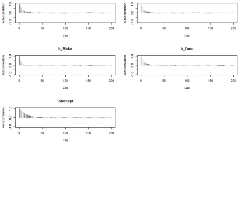
Autocorrelation is commonly defined as the degree of similarity between a given time-series and a lagged version of itself. Since the (i+ 1)th iteration depends only on the
ith iteration, autocorrelation is often quite high for Gibbs sampling. Autocorrelation with a
The high autocorrelation goes against the Gibbs sampler used. It is a strong indicator that running longer chains is required. Rather than thinning the chains and throwing away samples, the chains are ran for longer when autocorrelation is high as described in Sec-tion 2.7.1.
5
Results
In this chapter the results from all the methods employed are shown. To start, we model the expected claim frequency per year insured. Second, the expected claim severity per year insured. Finally, the expected compensation cost per year insured. The regression for each of the models are also given. Each model is analysed with residual analysis and scored with the DIC criterion. Trace plots and analysis for the MCMC chains are given.
5.1
Claim Frequency
5.1.1 Poisson Model
The Poisson model obtained after running 30,000 iterations of the Poisson is given by
E θi ti =exp(−1.89657 + 0.14532x1−0.10590x2 −0.19687x3−0.03691x4) (41)
Since this model, as with the other models given in this Section, is obtained by Bayesian inference, the posterior distribution can be directly examined to see which parameter val-ues are most credible. Unlike in frequentist statistical analysis, there is no need to gen-erate sampling distributions from null hypotheses and to figure out the probability that
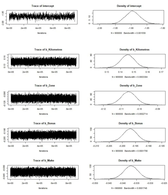
fictitious data would be more extreme than the observed data. In other words, there is no need for p values and p value based confidence intervals [Kruschke and Liddell, 2018]. Instead, measures of uncertainty are based directly on posterior credible intervals pro-vided in Table 5.3. The trace plots for the MCMC Gibbs samplers are given in Figure 5.1. We see that the criterion given by [Toft et al., 2007] listed in Section 2.7 are satisfied. The plots show that each variable mixed well, in that, it exhibits a rapid up and down variation with no long-term trends or drifts. The chain has mild correlation between draws and explores the sample space many times. Figure 5.1 gives both traceplots and density plots for the Poisson iterations. As true for all traceplots in this Section, traceplots repre-sent each sample step from the iterations ran. As each iterations jumps from one value to the next around the mean of the parameter, the traceplot allows for analysis of how well the parameter traveled in the state space. The traceplots do not show any significant changes in the target distributions. The density plots given in Figure 5.1 are the smoothed histograms of their respectful traceplots. That is to say, they represent the posterior distri-bution of the parameter. The normal curve is important for an accurate distridistri-bution about the mean.
HISTOGRAM
Furthermore, the autocorrelation plots are given in Figure 5.2. These plots support the likelihood of convergence from Figure 5.1. The relatively low autocorrelation after lag<50 suggests fast convergence for the model.
Figure 5.1: Trace Plots and Posterior Density Plots for Poisson Iterations. 3 Chains With 30,000 Iterations Each
Table 5.1: Poisson Heidelberg and Welch diagnostics
Stationarity and Half-width Test Start iteration P-value Mean Half-width
Intercept Passed 1 0.0772 -1.896 1.08e-03
Bonus Passed 1 0.7958 -0.197 8.05e-05
Kilometres Passed 24001 0.0574 0.145 1.91e-04
Make Passed 1 0.2974 -0.037 5.90e-05
Zone Passed 1 0.2728 -0.106 1.22e-04
Table 5.1 gives the Heidelberg and Welch diagnostics. All the variables passed the sta-tionarity and half-width test. Aside from kilometres, the variables all passed the stationar-ity test throughout the chain. The kilometres variables discarded the first 24,000 iterations of the chain before passing the stationarity test as described in Section 2.7.1. The large P-values obtained in the Heidelberg and Welch diagnostics are a good indication that the null hypothesis cannot be rejected and the chains are from a stationary distribution as described in Section 2.7.2. These p-values are not significant levels for the variables in the Poisson regression, but significance levels for the null hypothesis, the Gibbs sampling chains are from a stationary distribution.
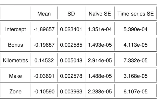
The results of the full MCMC iterations for all three chains is given in Table 5.2.
pos-Table 5.2: Poisson Posterior Results
Mean SD Na¨ıve SE Time-series SE
Intercept -1.89657 0.023401 1.351e-04 5.390e-04 Bonus -0.19687 0.002585 1.493e-05 4.113e-05 Kilometres 0.14532 0.005048 2.914e-05 7.332e-05
Make -0.03691 0.002578 1.488e-05 3.168e-05 Zone -0.10590 0.003963 2.288e-05 6.107e-05
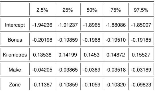
terior distribution calculated using the Poisson regression by means of Gibbs sampling. The posterior quantiles for each variable are given in Table 5.3. These are the confidence intervals for each estimated variable. From these results, it is seen that the Bonus and Kilometres have the most significant impact on the expected frequency. This is because the means for both of these variables are larger than their counterparts. Since the calcu-lations in Table 5.2 are calculated by taking the average across all iterations ran, the small standard deviation across all variables indicates a small dispersion of the data for each estimate of the model. The small standard error across the board indicates that the mean is a good reflection of the actual mean. The credible intervals for the lower and upper bounds of the parameter estimates are given in Table 5.3
Table 5.3: Poisson Credible Intervals 2.5% 25% 50% 75% 97.5% Intercept -1.94236 -1.91237 -1.8965 -1.88086 -1.85007 Bonus -0.20198 -0.19859 -0.1968 -0.19510 -0.19185 Kilometres 0.13538 0.14199 0.1453 0.14872 0.15527 Make -0.04205 -0.03865 -0.0369 -0.03518 -0.03189 Zone -0.11367 -0.10859 -0.1059 -0.10320 -0.09823
The 95% interval can be interpreted as the values between the 2.5% and 97.5% val-ues. For example, the 95% confidence interval for the Bonus coefficient is−0.20198to −
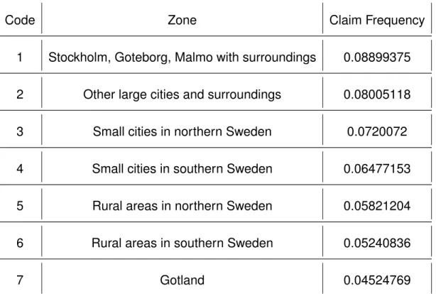
0.19185. Moving forward with the results, we can now interpret the expected claim fre-quencies per area. The results for the aforementioned are given in Table 5.4.
The inferences from the Poisson model, along with those of the other models as seen in the rest of Section 5, are in accordance with former knowledge of Claim frequencies. The results obtained from Table 5.4 are in keeping with what is expected. The higher claim frequencies come from larger cities with busier streets and more traffic. In the Appendix, Table 7.1 gives credible intervals for the claim frequency by zone. The average 95% error interval for the claim frequency by zone is 0.0191. The lower bound of the estimates vary by 13.73% from the mean, while the upper bound vary by 15.93% from the mean. For
fur-Table 5.4: Claim Frequency by Area (Poisson Results)
Code Zone Claim Frequency
1 Stockholm, Goteborg, Malmo with surroundings 0.08899375 2 Other large cities and surroundings 0.08005118
3 Small cities in northern Sweden 0.0720072
4 Small cities in southern Sweden 0.06477153
5 Rural areas in northern Sweden 0.05821204
6 Rural areas in southern Sweden 0.05240836
ther results, see Table 7.2 for the claim frequency by zone and kilometres driven. As the second practical check, the model is consistent with the data. Replicated data generated under the model does look similar to the previously observed data.
The residual plot for the Poisson model is analysed and given in Figure 5.3. The random pattern about zero represents the stochastic error of the model and indicates an appropri-ate fit from the Poisson model. The slightly positive trend in some of the residuals could be an indication of the strong influence the larger claim frequencies have on the model. The Poisson model is said to be over-dispersed, since the residual deviance/degrees of freedom is > 1. As is often the case with rare event count data, this suggests that the Poisson model is not the optimal model. Therefore, as previously mentioned in Section 5.1.3, the Negative Binomial model is analysed.
5.1.2 Zero-Inflated Poisson Model
The Zero-inflated Poisson model required many more iterations to achieve convergence. After running 300,00 iterations on 3 chains simultaneously, the model obtained is given by E θi ti =exp(−1.89501 + 0.14525x1 −0.10605x2−0.19699x3−0.03697x4). (42)
Equation (42) is the Zero-inflated regression model for the expected claim frequency per year of coverage. The slow convergence of the Markov chain can be caused by bad start-ing values, high posterior correlation, or under-parameterized models to name a few rea-sons. It is concluded that the slow convergence is a result of assuming no prior knowledge and the limited parameters for the model. In further work, the issue can be addressed with more data and prior knowledge to select informative priors.
As we can see from the Trace plots, all of the Zero-inflated Poisson variables mixed rather well aside from the intercept (β0). For this reason, the chains were run much longer to
ensure convergence.
The higher autocorrelation ofβ0was expected since it was slower to converge. However,
the chains still tend towards convergence as seen from the Heidelberg and Welch diag-nostic in Table 5.5. All variables passed both test and no iterations were discarded from the first half of the test. The large p-value from the intercept is a good indication that the null hypothesis cannot be rejected and the chains are from a stationary distribution.
Figure 5.4: Trace Plots and Posterior Density Plots for Zero-Inflated Poisson Itera-tions. 3 Chains With 300,000 Iterations Each
Table 5.5: Zero-Inflated Poisson Heidelberg and Welch diagnostics
Stationarity and Half-width Test Start iteration P-value Mean Half-width
Intercept Passed 1 0.974 -1.8962 3.17e-03
Bonus Passed 1 0.299 -0.1969 8.52e-05
Kilometres Passed 1 0.102 0.1454 1.81e-04
Make Passed 1 0.257 -0.0369 6.78e-05
Zone Passed 1 0.271 -0.1060 1.44e-04
Table 5.6: Zero-Inflated Poisson Posterior Results
Mean SD Na¨ıve SE Time-Series SE Intercept -1.89501 0.022828 2.406e-05 9.133e-04
Bonus -0.19699 0.002571 2.710e-06 2.500e-05
Kilometres 0.14525 0.004954 5.222e-06 5.340e-05 Make -0.03697 0.002559 2.697e-06 2.003e-05 Zone -0.10605 0.003973 4.187e-06 4.133e-05
Table 5.7: Zero-Inflated Poisson Credible Intervals 2.5% 25% 50% 75% 97.5% Intercept -1.93856 -1.9105 -1.89526 -1.87967 -1.85032 Bonus -0.20204 -0.1987 -0.19698 -0.19525 -0.19195 Kilometres 0.13556 0.1419 0.14526 0.14861 0.15497 Make -0.04196 -0.0387 -0.03698 -0.03525 -0.03194 Zone -0.11386 -0.1087 -0.10605 -0.10335 -0.09830 r (shape) 9.65539 10.61896 11.16488 11.73455 12.91373
The credible intervals are narrow with relatively small standard deviations as seen in Table 5.6. This signifies that the true estimation of the mean is relatively precise. See Table 5.8 for the results of the claim frequency from the Zero-inflated Poisson model.
The claim frequency results from the Zero-inflated model are comparable to the results obtained from the Poisson model. This indicates that the results are an appropriate fit since both models produced similar results. The data does not have enough zero-valued claims to have a noticeable improvement in the model and results. Therefore, a Zero-inflated model is not necessary since it has a much higher computing time to obtain the same results. Nevertheless, it is good to have a second model to complement the Poisson results. The 95% credible interval for the Zero-inflated Poisson model has an average