CALCULATION OF SOLVENCY CAPITAL REQUIREMENTS
FOR NON-LIFE UNDERWRITING RISK USING GENERALIZED
LINEAR MODELS
Jiří
1Valecký
*Abstract
The paper presents various GLM models using individual rating factors to calculate the solvency capital requirements for non-life underwriting risk in insurance. First, we consider the potential heterogeneity of claim frequency and the occurrence of large claims in the models. Second, we analyse how the distribution of frequency and severity varies depending on the modelling approach and examine how they are projected into SCR estimates according to the Solvency II Directive. In addition, we show that neglecting of large claims is as consequential as neglecting the heterogeneity of claim frequency. The claim frequency and severity are managed using generalized linear models, that is, negative-binomial and gamma regression. However, the different individual probabilities of large claims are represented by the binomial model and the large claim severity is managed using generalized Pareto distribution. The results are obtained and compared using the simulation of frequency-severity of an actual insurance portfolio.
Keywords: claim frequency, claim severity, generalized linear models, motor insurance, non-life insurance, solvency capital requirements, Solvency II, underwriting risk
JEL Classification: C31, C58, G22
1. Introduction
Differentiating premiums have been used in recent decades in the insurance sector. In motor hull insurance, the insurers usually set the annual premium to comply with the volume of the engine and the size of the district where the policyholder lives, although some insurers also consider the client’s age.
The collective risk model is mostly applied in non-life insurance. However, due to the increased use of premium differentiation, the application of individual risk models is important for pure premium calculation in which the annual premium is increasingly determined according to the relevant individual characteristics (rating factors). Furthermore, great importance is attached to individual risk models in credibility theory. Another important factor is the development of generalized linear models (GLMs), which have been studied intensively. In addition, the Directive 2009/138/EC (Solvency II) must be implemented in the legislation of EU member countries and takes effect in January 2016. This concept defines the solvency capital requirements (SCRs) in accordance with the total risk (market, credit, etc.) undertaken by the insurance company. It facilitates the use of full *1 Jiří Valecký, Faculty of Economics, Department of Finance, VŠB-TU Ostrava, Czech Republic
(jiri.valecky@vsb.cz).
This research was supported within the Project No. P403/12/P692 Managing and Modelling of Insurance Risks within Solvency II and within the Operational Programme Education for Competitiveness (Project No. CZ.1.07/2.3.00/20.0296).
The author would like to thank the anonymous reviewers for their valuable comments and suggestions to improve the quality of the paper.
or partial internal models in practice to calculate the expected losses and the SCRs. Some benefits of internal models were outlined in Liebwein (2006) and the future possibilities and validation were discussed by Brooks etal. (2009) and Eves and Keller (2013).
The developed models are mostly focussed on the calculation of SCRs and on the types of risk that are taken into account. The expected loss (or expected aggregated claims) of an insurance portfolio is mostly considered as input data, for example in the IAA model, IAA (2004), or it is a priori expected, for example in the Swiss Solvency Test, SST (2004). In addition, two approaches may be distinguished: (1) distribution-based models, IAA or SST, and (2) factor-based models, GDV model, GDV (2005), CEA model, CEA (2006) which significantly contributed to the debate on the concept of Solvency II. Good insights into the history of Solvency I/II are provided by Sandström (2006) and Sandström (2011), whereas Holzmüller (2009) compared Solvency II, American RBC standards, and SST.
The Solvency II takes effect in January 2016 and therefore there is a lack of studies focussed on assessing internal models. Some of them examine credit or equity risk, for example, Santomil et al. (2011), Gatzert and Martin (2012), Braun, Schmeiser, and Siegel (2014), or analyse the specific risks within the life underwriting risk (catastrophic or longevity risk), for example Kraut and Richter (2015). The unique study of SCR for non-life underwriting risk is the work of Jonas Alm, Alm (2015), who compares SCR generated by simulation model with different distributional assumptions with the standard formula. Some research also criticises the standard formula and derives recommendations for internal models, for example treating dependency between lines of business using copula functions, see Bermúdez, Ferri, and Guillén (2013).
In general, the internal model should be based on the calculation of aggregated claims and construction of the probability distribution which may be derived using classical risk theory – see Klugman et al. (2008), Mikosch (2009), Tse (2009) and many others – or by GLMs using individual rating factors. The latter approach (Frees, 2010, p. 429) is less extensive. The first regression analysis using individual rating factors and also one of the first separate analyses of claim frequency-severity appeared in Kahane and Levy (1975), while the first application of GLMs was used to model the claim frequency for marine insurance and the claim size for motor insurance in McCullagh and Nelder (1989). More applications of GLMs occurred mostly after the 1990s when the insurance market was being deregulated in many countries and the GLMs were used to perform a tariff analysis, for example in Brockman and Wright (1992), Andrade-Silva (1989) or Renshaw (1994).
Nowadays, the GLMs are used for undertaking tariff analysis, recently revised by David (2015), and setting the bonus-malus systems (BMSs) based on the credibility theory of Bühlmann (1967), or to set premiums, for example in Murphy et al. (2000), Zaks et al.
(2006) or Branda (2014). However, the complex approach using the empirical GLM to calculate SCR estimates is missing. This is the first study which proposes to use GLMs for SCR calculation. We consider this approach prospective and flexible because it reflects the (non-linear) dependency of individual risk on the individual rating factors and may yield a practical approach for SCR calculation.
Thus, we calculate SCR estimates for non-life underwriting risk using various GLM models which are based on individual rating factors. We also analyse the effect of GLM models considered in the distribution of severity and frequency and then examine how they are projected into SCR estimates according to the Solvency II Directive. The remainder of the paper is organized as follows. The general approach to capital requirements and
the fundamental features of Solvency II are described in Section 2. Section 3 focuses on the concept of GLMs, as well as describing applications to insurance data. The empirical results and comparisons of SCR estimates according to particular frequency-severity models are presented in Section 4. Section 5 provides the conclusions of this study.
2. Modelling Capital Requirements
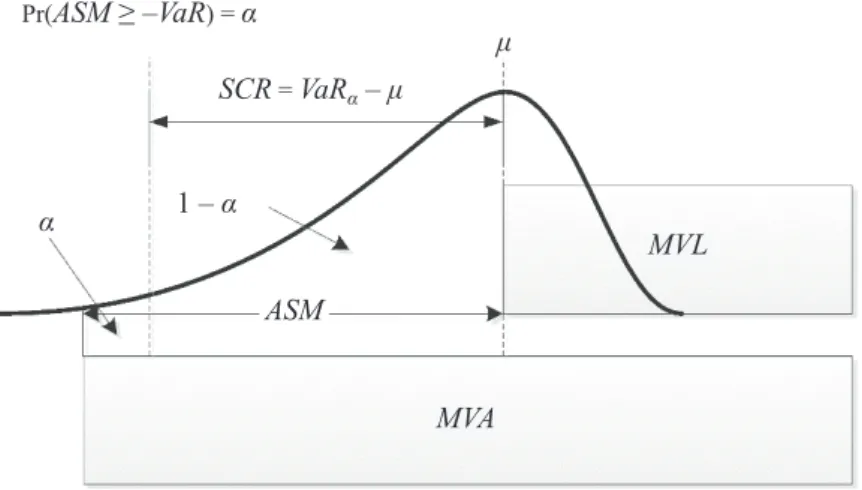
The general concept of modelling capital requirements implies that assets should cover all the obligations arising from business activities, not only of the insurance company. In other words, the market value of assets (MVA) should be higher than the market value of liabilities (MVL), that is, MVA≥MVL, and their difference could be set as the available solvency margin (ASM) intended to decrease the risk (or probability) that MVA < MVL over the given time horizon, as shown in Figure 1.
Figure 1 | Economic Approach to Solvency: The SCR Is Calculated as the Difference between the VaR and the Mean of the Distribution of ASM; the VaR Represents the Threshold Value, such that the Probability that ASM Exceeds this Value Is α
Source: Own elaboration of Sandström (2011, p. 62).
Solvency II is based on the same concept. The European Parliament passed the Frame-work Directive 2009/138/EC, which defines the solvency capital requirements (SCRs), in Article 101 as economic capital that absorbs losses at the 99.5% confidence interval over the 1-year risk horizon or 12 months, respectively. In addition, it defines the minimal capital requirements (MCRs) in Article 129 as the value at risk (VaR) subject to a confidence level of 85% over a 1-year risk period. It is clear that the government authorities will intervene if the solvency of a given insurance company falls below the MCR level.
According to the Framework Directive (FD) Article 101, the stated capital requirements must cover at least these risks; see Figure 2: 1) market risk, 2) credit risk, 3) operational risk, 4) non-life underwriting risk, 5) life underwriting risk and 6) health underwriting risk. In addition, CEIOPS (2009)1 proposed to calculate the SCRs for intangible assets risk.
1 Replaced by EIOPA in January 2011.
Pr(ASM ≥ –VaR) = α SCR = VaRα – μ 1 – α ASM MVL MVA α μ
Figure 2 | Classification of Risks in Solvency II
Source: Own representation.
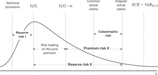
Figure 3 | Distribution of Aggregated Claims and Particular Risks within Solvency II
Source: Own representation.
By focussing on non-life underwriting risk, the FD requires the capital requirements to cover catastrophic risk (Article 105) and reserve and premium risk arising from obligations from existing contracts and new business expected to be written over the following 12 months. In addition, CEIOPS recommended respecting risk arising from options to
Premium risk Reserve risk II Reserve risk I Risk loading on the pure premium Catastrophic risk E[S] + m R E[S] Technical provisions Common actual claims u u i Irregular actual claimsm SCR=VaR99.5% S Reserve risk I Reserve risk II Risk loading on the pure premium Catastrophic risk Common actual claims Irregular actual claims Technical provisions SCR = VaR99.5% Premium risk II Reserve risk Premium risk Catastrophic risk Lapse risk
nate a contract before the maturity and options to renew the contract under the same condi-tions. This type of risk is known as lapse risk and it is taken into account in life insurance in general. However, this type of risk is involved in non-life insurance according to the 5th
Quantitative Impact Study (QIS5); see CEIOPS (2010) or EIOPA (2011).
Figure 3shows all the risks considered in Solvency II, namely the reserve, premium and catastrophic risk. Reserve risk is related to misestimated technical provisions (reserve risk I) and the stochastic nature of claims (actual claims fluctuate around the statistical mean value – reserve risk II). In contrast, the source of premium risk is the fact that the claims may be higher than the premiums received. Finally, catastrophic risk is represented by extreme or irregular events that are not captured by charges for premium and reserve risk.
3. Generalized Linear Models for Insurance Data
The key concept of all GLM models is the general exponential dispersion model. The GLMs particularities in non-life insurance risk modelling as well as the further details can be found in Jong and Heller (2008), Frees (2010) or Ohlsson and Johansson (2010).
3.1 Exponential dispersion model
The general exponential dispersion model uses a probability density function (pdf) with the form of
; ,
exp y
b
,
f y c y a , (1)where y is the response, θ is the location or mean parameter, b(θ) is the cumulant function,
ϕis the dispersion parameter and c(y, ϕ) is the normalization term. The choices of b(θ) and θ
determine completely the distribution of the model, however, the users prefer setting the probability distribution and the link function which yields the GLM model. The first and second derivatives of b(θ) with respect to θ give the mean response μ and its variance; thus
[ ] '( ) E y b , (2) '( ) ( ) ''( ) b ( ) V y b V , (3)
where V is the variance function (e.g. 1 for normal, μ for Poisson and μ2 for gamma
distribution). Some authors also specified a dispersion parameter as ϕ/w if they used grouped data, where w is the exposure. Then the pdf becomes
( ) ( ; , ) exp y b ( , , ) f y c y w w . (4)
However, the dispersion parameter is the same for all of the policyholders, while the parameter θ is allowed to depend on individual rating factors and it can be expressed as the systematic components ηi using the expression
0 1 1
i xi j ijx i g i
where xij is the j-th rating factor of the i-th policyholder, β are unknown parameters to be
estimated, g(.) is a known link function and the inverse link function is the mean function
μi = g−1 (ηi). If the equality g–1(ηi) = bʹ(θi) holds, the link function represents the canonical
link function and it follows that
θi = g(μi) = ηi = xiβ.
However, the function (5) is not necessarily a multivariate polynomial function of degree one. One of the techniques for handling higher non-integer degrees involves fractional polynomials (FPs), defined as follows:
0 1 1 2 2 1 ( )i K k k( )i i ... j ij k g F x x x
, (6)Where Fk (xi1) is a particular type of power function. The power pk could be any number, but
Royston and Altman (1994) restricted the power in the set S
–2; –1; –0.5; 0; 0.5; 1; 2; 3
, where 0 denotes the log of the variable. The remaining functions are defined as1 1 1 1 1 1 1 , , ( ) ( ) ln( ), k p i k k k i k i i k k x p p F x F x x p p (7)
for k = 1, …, K and restricting powers pk to those in S.
Finally, we note that the identification and comparison of the most appropriate FPs could be performed using the sequential procedure (Royston and Altman, 1994) or the closed test procedure (Marcus et al., 1976), of which the latter is generally preferred.
In addition, some rating factors in (5) may be interacted, which yields a systematic component written in the following form:
0 1 1 2 2 12 1 2 3 3
i x x x xi i xi j ijx
g( )i , (8)
where x1 and x2 are binary, categorical or continuous variables that are supposed to be
interacted.
Now, we consider the estimation of β parameters in general under the assumption of grouped data. Let the individual observations yi follow the exponential family
distri-bution (1) and be mutually independent, where the log-likelihood function of β estimates is
1 1 ( ) ( , ; ) N i i i i N ( , , ) i i i i w y b y c y w
(9)and the general first-order condition is in the form of
( ) 1 0 '( ) ( ) i i i ij i j i i y w x g V
. (10)To obtain the parameter estimates, we may employ two equivalent estimators: iteratively reweighted least squares based on Fisher scoring or the maximum likelihood Newton– Raphson-type algorithm. However, the latter might be preferable because the former must be amended using the observed information matrix instead of the expected information matrix if the non-canonical link function is used. Finally, the dispersion parameter ϕ can be estimated using the maximum likelihood method by solving 0 or by methods of moments
on the basis of Pearson 2( ) 1
x X N r
or deviance residuals ( ) 1
D D N r
, where
r is the number of parameters (including constants). McCullagh and Nelder (1989) and Meng (2004) performed some numerical experiments, which showed that calculations based on Pearson residuals are more robust against model error; thus, they recommended using ϕx.
3.2 Frequency-severity models
We may consider a Poisson regression model to model claim frequency. However, it is necessary to employ a model based on mixed Poisson distribution because it often experiences greater variance than that predicted by the model (known as over-dispersion or extra-Poisson variation). The gamma distribution is often used as the mixing distribution, which yields a negative-binomial (NB) model. It is also possible to assume other distributions, for example, inverse Gaussian or lognormal, which yield other types of the models. However, the parameter estimation process is complex and the improvements obtained are often only marginal (e.g. see Lemaire, 1991); therefore, the NB model is sufficient.
The claim severity based on the individual rating factors is mostly approximated using the gamma regression model, although large claims may occur. Practitioners cope with these problems by the truncation of claims. The threshold value for truncation is determined and the severity model is estimated for small-sized claims. Next, the pure premium is increased for each policy to obtain an adequate tariff. In other words, the expected aggregated claims generated by the GLM are equal to the observed total claims from the previous periods.
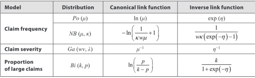
However, some policyholders may contribute to large claims differently and the pro-portion of large claims to the total loss could be estimated using the binomial logistic model while the claim count considers exposure. Table 1 shows some of the distributions that are suitable for frequency-severity models with canonical link functions and inverse functions.
Table 1 | Some of the Distributions from the Exponential Family
Model Distribution Canonical link function Inverse link function
Claim frequency Po (μ) ln (μ) exp (η) NB (μ, κ) ln 1 1 w
1 exp 1 w Claim severity Ga (wv, λ) μ−1 η−1 Proportion of large claims Bi (k, p) ln p k p 1 exp
k Source: Own.The models use the canonical link functions rarely in practice because beta restrictions are necessary; for example, the canonical link function for the NB model or the gamma model yields condition μi > 0, which implies xiβ < 0. Therefore, non-canonical functions
are used in practice; for example, the log link g (μi) = ln (μi) = xiβ with the inverse function μi = exp (xiβ) yields the NB2 model, which is mostly applied by practitioners (Hilbe, 2011,
3.3 Distribution of aggregate claims
To calculate the SCR for non-life underwriting risk, the distribution of aggregate claims (or total loss) S must be known. In general, the SCR is calculated as an α quantile, that is, VaR at given confidence level α, thus
( ) inf : S( )
VaR s s R F s , (11)
where FS (s) is the cumulative distribution function (cdf) of total loss.
Let FiS, FG be the cdf of small and large claim severity; the cdf of the individual claim of the
i-th policyholder can be written as the cdf of mixture distribution with the form of
(1 )
i
X i iS i G
F p F p F , (12)
where pi is the mixing binomial probability, FiS is the cdf of gamma distribution from Table 1
and FG is the cdf of generalized Pareto distribution (GPD) with the shape parameter k≠ 0,
the scale parameter σ and the threshold (location) parameter θ and takes the following form:
1 1 1 k G x F k . (13)By focussing on the distribution of individual claims of all of the policyholders, we obtain the cdf of compound distribution:
0 Pr( ) i i n L X i n F F N n
, (14)which is a countable mixture of 0
i X
F, 1
i X
F, … with mixing proportions Pr (N
i = 0), Pr (Ni = 1),
… and where *n is n-fold convolution.
Finally, the cdf of total loss may be derived as a convolution of (13) for all of the policyholders as follows:
1
( *...* n)
S L L
F F F . (15)
4. Empirical Results for a Motor Hull Insurance Portfolio
In this section, we calculate SCR estimates using several GLMs and we evaluate their impact on claim frequency-severity distribution. We also provide an insight into how the SCR estimates for non-life underwriting risk of a motor hull insurance portfolio vary according to the frequency-severity models. The parameter estimates were obtained using STATA 12.1 and we used our own Matlab codes to simulate the frequency-severity of the insurance portfolio.
The data sample encompassed the characteristics of the given motor hull insurance portfolio during the years 2005–2008 (220,022 observations) when 14,166 claims occurred. The known explanatory variables (rating factors) are the following: vehicle age (agecar), engine power divided by engine volume (kwvol), owner’s age (ageman), vehicle price
(price), indicator of company/private car (company), gender of policyholder (gender), type
of fuel (fuel), district area (district) and time exposition (duration). The portfolio used for SCR calculation was supposed to be made up of 63,178 policies.
First, we obtained parameter estimates of the model for claim severity without dis-cerning small and large claims and we built the model considering the occurrence of ex-treme claims. Then, we considered that each policy contributed to the total loss differently and we used a binomial logistic regression model to calculate the probability of large claims. The large claim severity was treated using risk theory by estimating the GPD. We also demonstrated the practical approach (see Ohlsson and Johansson, 2010, p. 64), which consisted of artificially increasing the constant parameter of the claim severity or frequency model to point out the difference from the view of the statistical approach.
Second, we estimated the parameters of several types of NB2 models for claim frequency: (a) linear (with a linear link function), (b) non-linear (with a non-linear link function involving FPs) and (c) non-linear interacting models. Further, we combined these models with models for claim severity in which the large claims were considered. All the parameters were obtained using the maximum likelihood estimator and the estimated scale parameters were calculated using the Pearson chi-squared residuals.
Finally, to analyse the impact of the modelling techniques on the distributions, we avoided analytical and numerical solutions because of their complexity and we relied on simulation-based experiments. Due to the enormous number of scenarios that were necessary to obtain reliable results (at least 100,000 scenarios for each of 63,178 policies) and to keep the simulation error small, we generated only 10,000 scenarios for each policy using pseudo-random numbers generated by the linear congruential generator (LCG) and we used the Latin hypercube sampling (LHS) algorithm. The simulated individual claims were aggregated in the distribution of the total expected loss for the motor hull insurance portfolio and particular SCR estimates according to all the models considered in this study were calculated and compared.
4.1 Distribution of claim severity
Although a non-linear impact of rating factors on claim severity occurs, only the linear model for claim severity was considered because we believe that the non-linearity cannot be supported in rational terms. To reflect the occurrence of large claims in the model, the truncation level was determined subjectively using pre-analysis at the level of 67,000. This level ensured sufficient data to estimate the large claim distribution and to obtain a tariff that could be easy to sell. Thus, a new variable sizeAdj = min (size,c) was created, where c
is the threshold value for truncation, size is the original claim and sizeAdj is the truncated claim. Figure 4 shows the empirical histograms of the original and truncated data, in which the low probability of small claims is evident.
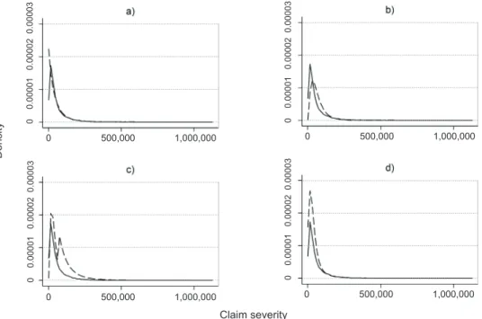
Then, we modelled the individual claim severity using the various regression models: (1) the gamma model without truncation; (2) the truncated gamma model with an adjusted intercept in which the intercept had to be increased by 0.2346 to distribute the costs above the truncation level; (3) the gamma model combined with the GPD (without mixing probabilities); and (4) the truncated mixed model (gamma and GPD). In the mixed model, we considered the individual probabilities of large claims using the binomial logistic regression model, in which the same explanatory rating factors were used while the number of claims that exceeded the truncation level was considered as the outcome and the claim count was used as the exposure. The large claim severity was assumed to follow the GPD. Figure 5 compares the estimated density and averaged density obtained using these approaches.
Figure 4 | Histograms of Empirical Severity: The Left Panel Represents All of the Observations and the Right Panel Depicts the Truncated Data
Source: Own calculations; Stata 12.1.
Figure 5 | Estimated (solid line) and Averaged Density (dashed line) of Claim Severities:
(a) The Gamma Regression without Truncation, (b) The Truncated Gamma Regression with the Adjus- ted Intercept, (c) The Truncated Gamma Model with the GPD and (d) the Truncated Mixed Model
Source: Own calculations; Matlab R2010b.
Clearly, the gamma model without truncation overestimated the probabilities of small claims, while the gamma model with the adjusted intercept underestimated them. On the other hand, the approaches that combined the gamma distribution and the GPD appeared to fit the data better, but the truncated gamma model with GPD yielded a bimodal distribution. However, they overestimated the probability of medium-sized claims because the GPD overestimated the probabilities of claims above 67,000. Thus, the GPD did not fit the data
Density Claim severity Empirical severity Density 1,000,000 0 500,000 1,000,000 0 500,000 1,000,000 0 0.00001 0.00002 0.00003 0 0.00001 0.00002 0.00003 0 0.00001 0.00002 0.00003 0 0.00001 0.00002 0.00003 0 500,000 1,000,000 0 500,000 1,000,000 0 500,000 1,000,000 0 20,000 40,000 60,000 80,000
1.0e-05 2.0e-05 3.0e-05
sufficiently. Nonetheless, this study was not focussed on this issue and we recommend the mixed model, which represented the statistical nature of claim severity, the most.
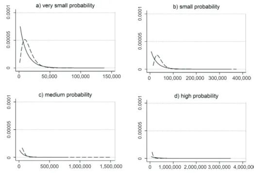
Figure 6 shows some of the individual distributions of claim severity, while Table 2 presents some descriptive statistics to demonstrate the differences in claim severity distributions between the gamma and the mixed model for some policyholders with various probabilities of large claim occurrence.
Figure 6 | Density of Simulated Severity of Given Policyholders: Gamma Model (solid line) and Truncated Mixed Model (dashed line)
Source: Own calculations; Matlab R2010b.
Comparing the gamma and mixed models, the gamma model overstated the probability of small claims. In addition, the gamma model did not reflect the small probabilities of small-sized claims at all, while the mixed model respected this phenomenon except for medium and high probabilities of large claim occurrence. It was caused mainly by the threshold value, which was determined subjectively at the same level for all of the policies and which yielded increasing use of the GPD to fit the claim severity instead of the gamma distribution. Table 2 shows some descriptive statistics of the claim severity distributions generated by the gamma and mixed models.
By comparing the descriptive statistics, we can see that the mixed model predicted greater expected value (mean) except for the policy with a high probability of large claim occurrence. In addition, the variance was reduced enormously, especially for the medium and high probabilities. Finally, the ninety-fifth and ninety-ninth percentiles of the mixed model are significantly smaller than the percentiles of the gamma model.
Density Simulated severity 0 100,000 200,000 300,000 400,000 0 0.00005 0.0001 0 0.00005 0.0001 0 0.00005 0.0001 0 0.00005 0.0001 0 1,000,000 2,000,000 3,000,000 4,000,000 0 500,000 1,000,000 1,500,000 0 50,000 100,000 150,000
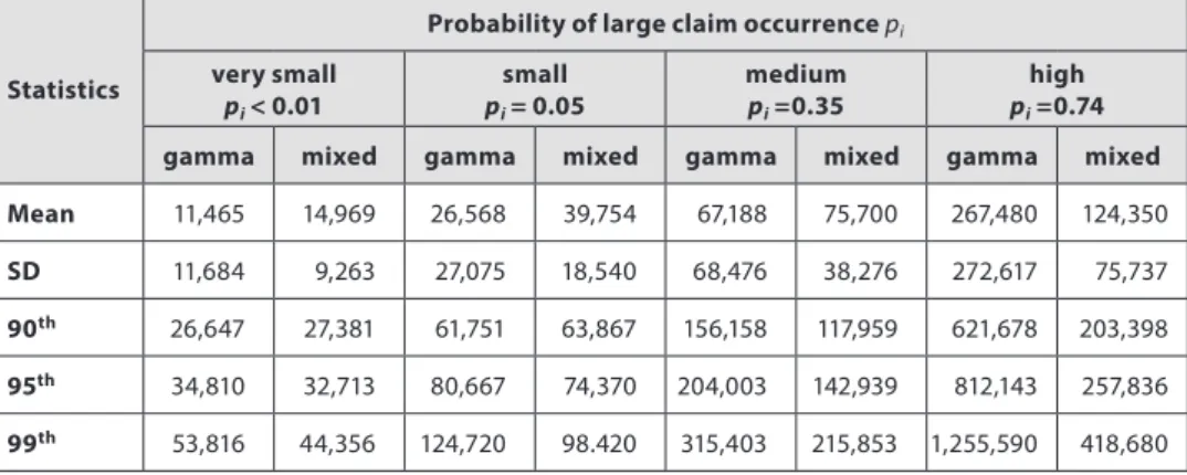
Table 2 | Some Descriptive Statistics of Claim Severity Distributions with Various Probabilities of Occurrence of Large Claims
Statistics
Probability of large claim occurrence pi
very small pi< 0.01 small pi= 0.05 medium pi =0.35 high pi =0.74
gamma mixed gamma mixed gamma mixed gamma mixed
Mean 11,465 14,969 26,568 39,754 67,188 75,700 267,480 124,350
SD 11,684 9,263 27,075 18,540 68,476 38,276 272,617 75,737
90th 26,647 27,381 61,751 63,867 156,158 117,959 621,678 203,398
95th 34,810 32,713 80,667 74,370 204,003 142,939 812,143 257,836
99th 53,816 44,356 124,720 98.420 315,403 215,853 1,255,590 418,680
Source: Own calculations; Matlab R2010b.
These results influence the premium calculation using the equivalence principle because the higher expected value means higher premiums. On the contrary, the reduced variance implies smaller risk loadings, which yield lower premiums. It depends on which effect prevails. However, the mixed model decreased the differentiation of expected severity and the premiums, although this model involved the occurrence of large claims. In addition, the mixed model may provide a tariff that would be easier to sell compared with the tariffs obtained using the gamma model.
4.2 Distribution of claim frequency
Now, we focus on modelling the claim frequency. We estimated three negative-binomial models: (1) linear, (2) non-linear involving fractional polynomials and (3) non-linear with interactions between some rating factors. The non-linearity was identified for
ageman, agecar, kwvol and price with FP powers of (2 2) for kwvol, (−2 3) for ageman,
(0.5 1) for agecar and (0.5 0) for price. The interactions were considered only between
gender × ageman and company × fuel because only these appeared to be reasonable and
may be supported in practical terms.
In general, the reason why the Poisson regression does not fit the data sufficiently is the heterogeneity that occurs among policyholders. Our results also confirmed this phenomenon; see Table 3, in which the Poisson model is compared with the NB2 model.
The results show that the Poisson model overestimated the probabilities of zero count and underestimated the probabilities of one insured accident. In contrast, the NB2 model fitted the observed probabilities better. The probabilities generated by the other types of NB2 models are not presented here because the differences were very small and we assess their impact on the SCR estimates in the next section. Table 4 shows the comparison of the descriptive statistics of the observed and predicted frequencies as well as the estimated scale and dispersion parameters.
The results show the minimal impact of higher complexity of the model. The impact of the model on the predicted claim frequency depended on the estimated mean and the scale
parameter, which varied significantly across the models. Thus, the more complex model yielded higher probabilities of non-zero claim count.
Table 3 | Observed and Predicted Probabilities (%)
Count Observed probability
Predicted probability Difference
Poisson Linear NB2 Poisson NB2
0 93.562 93.348 93.603 0.214 −0.042
1 5.933 6.327 5.828 −0.393 0.105
2 0.459 0.312 0.505 0.147 −0.046
3 0.044 0.013 0.055 0.031 −0.011
4 0.002 0.001 0.007 0.002 −0.005
Source: Own calculations; Matlab R2010b.
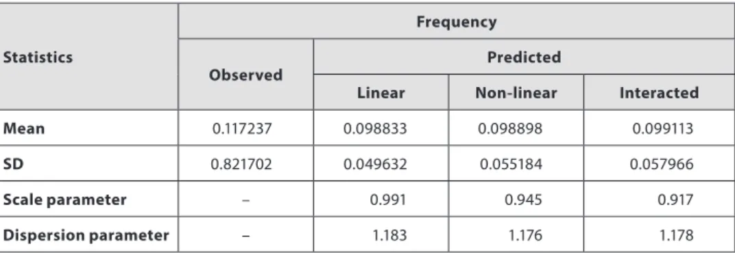
Table 4 | Observed and Predicted Claim Frequency
Statistics
Frequency
Observed
Predicted
Linear Non-linear Interacted
Mean 0.117237 0.098833 0.098898 0.099113
SD 0.821702 0.049632 0.055184 0.057966
Scale parameter – 0.991 0.945 0.917
Dispersion parameter – 1.183 1.176 1.178
Source: Own calculations; Stata 12.1.
In addition, the standard deviation of expected claim frequencies increased significantly when the more complex model was used; therefore, the importance of the models consisted of increased differentiation of the expected claim frequency among policies. Finally, the estimated dispersion parameter does not vary significantly and it indicates that all of the frequency models suffer over-dispersion.
4.3 Distribution of aggregated claims and SCR estimates
Finally, we estimated the MCR and SCR for non-life underwriting risk for a motor hull insurance portfolio for all the types of the models considered. We simulated the claim frequency and severity for each policy of the insurance portfolio. Because we focussed on capital requirements, Figure 7 shows only the upper tails of the distributions of the aggregated claims.
It is clear that the mixed severity model combined with the negative-binomial models gave the highest estimates of capital requirements. The truncated severity models with adjusted frequency or severity understated the estimates by approximately 60–80 million.
These models were calibrated on the expected truncated claims with increased base frequency or base severity and these models do not respect statistical nature of frequency-severity at all. In addition, we point out the issue of determining whether to increase the base frequency or base severity. However, considering the last observed total loss of the insurance portfolio at the level of 217 million, the capital requirements determined by all of the models covered this loss.
Figure 7 | Upper Tails of the Distributions for Various Models: Severity Models Combined with the NB2 Frequency Model (left panel) and Different Claim Frequencies Combined with the Mixed Severity Model (right panel)
Source: Own calculations; Matlab R2010b.
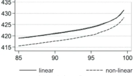
By comparing the results determined by the various frequency models, we found that the SCR estimates did not differ significantly, as shown in Table 5, in which the results of the Poisson model are also recorded.
Table 5 | MCR and SCR Estimates according to the Models (mil. of CZK)
Claim severity model Gamma Mixed
Claim frequency model Linear Linear Non-linear Interacted
non-linear Poisson Percentile MCR 85.0 378.98 418.94 415.55 419.05 380.82 90.0 380.87 420.93 417.69 421.18 382.74 95.0 383.76 423.62 420.28 423.88 385.37 SCR 99.5 391.20 431.40 428.04 431.34 392.90
Source: Own calculations; Matlab R2010b.
We highlight that neglecting the heterogeneity of claim frequency (i.e. the Poisson model) gave similar SCR estimates as the gamma model combined with the NB2 model. Comparing all the results, the approach that combined the mixed model and any NB2 model yielded the highest SCR estimates. However, the differences between them were negligible and the importance of the complexity of the claim frequency model consisted rather of the differentiation of the premium than of the determination of significantly different SCR estimates. Percentile Total loss interacted non-linear non-linear linear mixed adj. freq. gamma adj. sev.
5. Conclusion
In this study, we calculated SCR estimates for non-life underwriting risk using several GLMs and we evaluated their impact on the distribution of individual claim severity and claim frequency. We also provided insights into how these models influenced the distri-bution of aggregated loss and how the SCR estimates for non-life underwriting risk of a motor hull insurance portfolio varied across the frequency-severity models.
As a result, we concluded that the probabilities of small claims were underestimated if the severity was approximated by the gamma model, in which the small and large claims were not discerned. We also did not recommend the practical approach using the calibration of frequency-severity models. In addition to the question of increasing the base frequency or the base severity, these models do not respect the statistical nature of frequency-severity. However, all the models covered the last observed loss sufficiently, although the GPD distribution did not fit the empirical severity perfectly. Furthermore, the mixed model decreased the differences among the estimated severities, which yielded reduced volatility. As an inference, it might be utilized in premium pricing by setting higher expected an individual loss and smaller risk loading parameters.
The estimated claim frequency was also affected by the frequency model used. However, the effect of the model complexity consisted of increased differentiation of expected frequencies across policies rather than significant differences in SCR estimates. In other words, if we respected non-linearity or interactions, we did not obtain significantly different SCR estimates. Furthermore, these frequency models were more important for the individual claim estimates and setting the premium. By comparing the SCR estimates determined by the frequency-severity models, we identified that neglecting the heterogeneity in claim frequency (i.e. using the Poisson model) was as consequential as neglecting the occurrence of large claims. Finally, the approach combining the mixed model and any negative-binomial model yielded the highest SCR estimates.
Thus, the next research should be devoted to improving the fit of the large claim severity. It would be possible to develop the Pareto regression model to fit individual large claim severity better or to use another proper type of distribution. Furthermore, identifying the individual truncation level to obtain a better-fitted model would be very helpful. Finally, the catastrophic risk was incorporated into our study in terms of individual severity, not in terms of the occurrence of several claims during a short period, which involves the mutual dependence among policies and violates the central limit theorem.
References
Alm, J. (2015). A Simulation Model for Calculating Solvency Capital Requirements for Non-Life Insurance Risk. Scandinavian Actuarial Journal, 2015(2), 107–123, https://doi.org/10.1080/ 03461238.2013.787367
Andrade-Silva, J. M. (1989). An Application of Generalized Linear Models to Portuguese Motor Insurance. Proceedings XXI ASTIN Colloquium. New York: N.p. 633.
Bermúdez, L., Ferri, A., Guillén, M. (2013). A Correlation Sensitivity Analysis of Non-Life Underwriting Risk in Solvency Capital Requirement Estimation. ASTIN Bulletin, 43(01), 21–37, https://doi.org/10.1017/asb.2012.1
Branda, M. (2014). Optimization Approaches to Multiplicative Tariff of Rates
Estimation in Non-Life Insurance. Asia-Pacific Journal of Operational Research, 31(5), 1450032 (17 pages), https://doi.org/10.1142/s0217595914500328
Braun, A., Schmeiser, H., Siegel, C. (2014). The Impact of Private Equity on a Life Insurer’s Capital Charges under Solvency II and the Swiss Solvency Test. Journal of Risk and Insurance, 81(1), 113–158, https://doi.org/10.1111/j.1539-6975.2012.01500.x
Brockman, M. J., Wright, T. S. (1992). Statistical Motor Rating: Making Efficient Use of Your Data. Journal of the Institute of Actuaries, 119(03), 457–543, https://doi.org/10.1017/ s0020268100019995
Brooks, D. et al. (2009). Actuarial Aspects of Internal Models for Solvency II. British Actuarial Journal, 15(02), 367–482, https://doi.org/10.1017/s1357321700005705
Bühlmann, H. (1967). Experience Rating and Credibility. ASTIN Bulletin, 4(03), 199–207, https:// doi.org/10.1017/s0515036100008989
CEA (2006). CEA Working Document on the Standard Approach for Calculating the Solvency Capital Requirement. 22 March 2006.
CEIOPS (2009). CEIOPS’ Advice for L2 Implementing Measures on SII: Classification and Eligibility of Own Funds. Former Consultation Paper No. 46.
_______ (2010). QIS5 Technical Specifications. 5 July 2010.
EIOPA (2011). EIOPA Report on the Fifth Quantitative Impact Study for Solvency II. 14 March 2011. Eves, M., Keller, P. (2013). What Solvency II Firms Can Learn from the Swiss Solvency Experience.
British Actuarial Journal, 18(03), 503–522, https://doi.org/10.1017/s1357321713000305 Frees, E. W. (2010). Regression Modeling with Actuarial and Financial Applications. New York:
Cambridge University Press.
Gatzert, N., Martin, M. (2012). Quantifying Credit and Market Risk under Solvency II: Standard Approach versus Internal Model. Insurance: Mathematics and Economics, 51(3), 649–666, https://doi.org/10.1016/j.insmatheco.2012.09.002
GDV (2005). Discussion Paper for a Solvency II Compatible Standard Approach (Pillar I) Model Description. Berlin: GDV.
Hilbe, J. M. (2011). Negative Binomial Regression. Cambridge: Cambridge University Press. Holzmüller, I. (2009). The United States RBC Standards, Solvency II and the Swiss Solvency Test:
A Comparative Assessment. The Geneva Papers on Risk and Insurance - Issues and Practice, 34(1), 56–77, https://doi.org/10.1057/gpp.2008.43
IAA (2004). A Global Framework for Insurer Solvency Assessment. International Actuarial Association.
Jong, P. de, Heller, G. Z. (2008). Generalized Linear Models for Insurance Data. Cambridge: Cambridge University Press.
Kahane, Y., Levy, H. (1975). Regulation in the Insurance Industry: Determination of Premiums in Automobile Insurance, Journal of Risk and Insurance, 42(1), 117–132, https://doi. org/10.2307/251592
Klugman, S. A., Panjer, H. H., Willmot, G. E. (2008). Loss Models: From Data to Decisions. Hoboken: John Wiley & Sons.
Kraut, G., Richter, A. (2015). Insurance Regulation and Life Catastrophe Risk: Treatment of Life Catastrophe Risk under the SCR Standard Formula of Solvency II and the Necessity of Partial Internal Models. The Geneva Papers on Risk and Insurance - Issues and Practice, 40(2), 256–278, https://doi.org/10.1057/gpp.2014.10
Lemaire, J. (1991). Negative Binomial or Poisson-Inverse Gaussian? ASTIN Bulletin, 21, 167–168. Liebwein, P. (2006). Risk Models for Capital Adequacy: Applications in the Context of Solvency II
and beyond. The Geneva Papers on Risk and Insurance - Issues and Practice, 31(3), 528–550, https://doi.org/10.1057/palgrave.gpp.2510095
Marcus, R., Peritz, E., Gabriel, K. R. (1976). On Closed Test Procedures with Special Reference to Ordered Analysis of Variance. Biometrika, 63(3), 655–660, https://doi.org/10.2307/2335748 McCullagh, P., Nelder, J. A. (1989). Generalized Linear Models. 2nd Edition. London: Chapman
& Hall.
Meng (2004). Estimation of Dispersion Parameters in GLMs with and without Random Effects. Dissertation. Stockholm University.
Mikosch, T. (2009). Non-Life Insurance Mathematics: An Introduction with the Poisson Process. Berlin Heidelberg: Springer.
Murphy, K. P., Brockman, M. J., Lee, P. K. W. (2000). Using Generalized Linear Models to Build Dynamic Pricing Systems for Personal Lines Insurance. Casualty Actuarial Society Forum. Ohlsson, E., Johansson, B. (2010). Non-Life Insurance Pricing with Generalized Linear Models.
Berlin: Springer. EAA Series.
Renshaw, A. E. (1994). Modelling the Claims Process in the Presence of Covariates. ASTIN Bulletin, 24(02), 265–285, https://doi.org/10.2143/ast.24.2.2005070
Royston, P., Altman, D. G. (1994). Regression Using Fractional Polynomials of Continuous Covariates: Parsimonious Parametric Modeling. Applied Statistics, 43(3), 429–467, https:// doi.org/10.2307/2986270
Sandström, A. (2011). Handbook of Solvency for Actuaries and Risk Managers : Theory and Practice. Boca Raton: CRC Press.
___________ (2006). Solvency: Models, Assessment and Regulation. Boca Raton: Chapman & Hall/CRC.
Santomil, P. D. et al. (2011). Equity Risk Analysis in the Solvency II framework: Internal Models versus the Standard Model. Cuadernos de Economía y Dirección de la Empresa, 14(2), 91–101, https://doi.org/10.1016/j.cede.2011.02.003
SST. (2004). The Risk Margin for the Swiss Solvency Test. Federal Office for Private Insurance, Bern, September 17.
Tse, Y.- K. (2009). Nonlife Actuarial Models : Theory, Methods and Evaluation. Cambridge: Cambridge University Press.
Zaks, Y., E. Frostig, B. Levikson. (2006). Optimal Pricing of a Heterogeneous Portfolio for a Given Risk Level. ASTIN Bulletin, 36(1), 161–185, https://doi.org/10.2143/ast.36.1.2014148