Nikolay Robinzonov, Gerhard Tutz & Torsten Hothorn
Boosting Techniques for Nonlinear
Time Series Models
Technical Report Number 075, 2010
Department of Statistics
University of Munich
Boosting Techniques for Nonlinear Time Series Models
Nikolay Robinzonov
1Gerhard Tutz
1Torsten Hothorn
1,∗1Institut f¨ur Statistik, Ludwig-Maximilians-Universit¨at M¨unchen
Ludwigstraße 33, D–80539 M¨unchen, Germany
Abstract
Many of the popular nonlinear time series models requirea priorithe choice of parametric
functions which are assumed to be appropriate in specific applications. This approach is used mainly in financial applications, when sufficient knowledge is available about the nonlinear structure between the covariates and the response. One principal strategy to investigate a broader class on nonlinear time series is the Nonlinear Additive AutoRegressive (NAAR) model. The NAAR model estimates the lags of a time series as flexible functions in order to detect non-monotone relationships between current observations and past values. We consider linear and additive models for identifying nonlinear relationships. A componentwise boosting algorithm is applied to simultaneous model fitting, variable selection, and model choice. Thus, with the application of boosting for fitting potentially nonlinear models we address the major issues in time series modelling: lag selection and nonlinearity. By means of simulation we compare the outcomes of boosting to the outcomes obtained through alternative nonparametric methods. Boosting shows an overall strong performance in terms of precise estimations of highly nonlinear lag functions. The forecasting potential of boosting is examined on real data where the target variable is the German industrial production (IP). In order to improve the model’s forecasting quality we include additional exogenous variables. Thus we address the second major aspect in this paper which concerns the issue of high-dimensionality in models. Allowing additional inputs in the model extends the NAAR model to an even broader class of models, namely the NAARX model. We show that boosting can cope with large models which have many covariates compared to the number of observations.
keywords: componentwise boosting, forecasting, nonlinear times series, autoregressive additive models, lag selection.
∗Corresponding author. Email: [email protected], Tel.: +49 89 2180 6407,Fax: +49 89
1 INTRODUCTION
1 Introduction
An essential property of a time series is its unknown evolution over time. Some paths are more probable than others and this motivates researchers to try to understand the data generating process and possibly to forecast future events. Linear models provide a starting point for modelling the nature of time series. Linear time series models, however, encounter various limitations in the real world and are applicable only under very restrictive conditions. The field of time series has witnessed various new developments in the past two decades which has relaxed some of these constraints. In particular, the development of nonparametric regression added more flexibility to standard linear regression adopted by the time series paradigm, see for example Lewis and Stevens (1991), Chen and Tsay (1993), or Huang and Yang (2004). A leading aspect to be explored throughout this paper is the nonparametric modelling and the resulting forecasting techniques.
The second major aspect concerns the issue of high-dimensionality in the models, i.e., models taking potentially many covariates into account. Boosting, one of the most influential strategies that deal with high-dimensional models, has its roots in machine learning. The idea has undergone significant evolution in the last decade. It has been successfully applied to statistical model fitting (e.g., B¨uhlmann and Hothorn, 2007). The novel component of the present work is the application of boosting to time series, where nonlinear functions of lagged values of a time series have to be estimated.
Due to the frequent use of the simple univariate autoregressive model (AR), we draw on it as a benchmark in the application part to follow. For a substantially broader discussion on times series, see Hamilton (1994). In addition we consider thevector autoregressive (VAR) model. The VAR model suggests that every variable is a linear combination of its past observations and the past observations of supplemental variables. In practice such assumptions enjoy great popularity. Multivariate time series are considered in greater depth by L¨utkepohl (1991, 2006).
The literature offers a great amount of nonlinear modelling tools. Many of them are developed in the spirit of nonlinearparametric models. They require an a priori choice of parametric functions, which are assumed to be appropriate in specific situations. That approach is used mainly in financial applications, when sufficient knowledge is available about the nonlinear structure between the covariates and the response. However, the appropriateness of such assumptions is usually hard to justify in practice.
In contrast to parametric nonlinear models, nonparametric techniques are not restricted to a particular choice of parametric functions. One principal strategy is to study the times series counterpart of the additive model; the so-calledNonlinear Additive AutoRegressive(NAAR) model (Chen and Tsay, 1993). When further (exogenous) variables are available, we suitably extend the model with more functions and call it NAARX (Chen and Tsay, 1993). Thus, NAARX encompasses linear regressive models and many nonlinear models as special cases.
The literature on nonlinear additive models is extensive, therefore, we concentrate on nonpara-metric approaches. Huang and Yang (2004) recently introduced a method that attracted much attention because of appealing lag-selection properties for univariate nonlinear time series. It es-sentially represents an additive version of thelinear stepwise procedure using truncated splines or B-Splines as base expansions of the predictors. The proposed base functions are not penalized. Instead, a formula is suggested which determines a relatively small number of evenly spaced knots. In terms of lag selection, the proposed method performed quite well with simulated time series. However, no results were provided that show the goodness-of-fit of models. We will use some of the artificial times series, provided by Huang and Yang (2004) in Section 3.2 and will shed light upon
2 BOOSTING LINEAR AND ADDITIVE MODELS the goodness-of-fit as well.
Multivariate Adaptive Regression Splines (MARS) were introduced by Friedman (1991). A neat overview of the method is available in Hastie et al. (2001), Hastie, Tibshirani and Friedman (2009, Chapter 9) and an application of MARS in a time series context is provided by Lewis and Stevens (1991). The last nonparametric model that we consider is the BRUTO procedure (Hastie and Tibshirani, 1990, Chapter 9). BRUTO combines inputs selection with backfitting by using smoothing splines. It was applied to time series by Chen and Tsay (1993). See Hastie and Tibshirani (1990, p. 90-91) for details concerning backfitting and Hastie and Tibshirani (1990, p. 262) for the BRUTO algorithm.
We proceed as follows. In Section 2, we shortly review the general ideas of boosting. We adopt the statistical view on boosting, which is considered purely a numerical optimization, rather than a “traditional” statistical model. Exemplified by two weak learners, we examine the structure of the boosting algorithm for continuous data. The first weak learner is a simple linear models, the second weak learner is a penalized B-Spline (Eilers and Marx, 1996).
Section 3 examines the results of a simulation study. We analyze the performance of boosting with P-Spline weak learners in Monte Carlo simulations with six artificial, nonlinear, autoregressive time series. We compare the outcomes of boosting to the outcomes obtained through alternative nonparametric methods. Their performances are considered in terms of lag-selection and goodness-of-fit.
In Section 4 we apply boosting, both with linear and additive learners, to real world data in terms of forecasting. The target variable is the German industrial production. We compare boosting, along with other methods, to the simple univariate autoregressive model.
2 Boosting Linear and Additive Models
Boosting, in its famous AdaBoost formulation, was developed by Freund and Schapire (1996). Friedman (2001) embedded this algorithm into the framework of functional gradient descent opti-mization for function estimation and made connections to statistical model fitting, for example to logistic regression. B¨uhlmann and Yu (2003) established componentwise boosting as a means of fitting generalized linear and additive models. This seminal paper showed that boosting procedures can be used to fit a huge class of classical and modern statistical models. For an overview on boosting in general we refer to B¨uhlmann and Hothorn (2007).
2.1 Steepest Descent
The statistical framework developed by Friedman (2001) interprets boosting as a method for direct function estimation. He shows that boosting can be interpreted as a basis expansion, in which every single basis term is iteratively refitted. Still, some care must be taken in interpreting boosting as a basis expansion. In contrast to conventional basis expansions, where the basis functions are known in advance, the basis’s members and also their number are iteratively determined by the fitting procedure. Our notation is as follows:
zt= (y>t ,x>t )>= (yt−1, . . . , yt−p, x(1)t−1, . . . , x(1)t−p, . . . , x(tq−)1, . . . , xt(−q)p)>∈R(q+1)p
denotes thep-lagged vector of explanatory variables representing the lagged valuesyt= (yt−1, . . . , yt−p)>∈ Rpof the endogenous variabley
2.1 Steepest Descent 2 BOOSTING LINEAR AND ADDITIVE MODELS proposed model is then
E(yt|zt) = p X i=1 fi(yt−i) + p X i=1 fi(1)(x(1)t−i) +· · ·+ p X i=1 fi(q)(x(tq−)i) = p X i=1 fi(yt−i) + q X j=1 p X i=1 fi(j)(xt(j−)i) =:F(zt). (NAARX)
The objective is to obtain an estimate ˆF of the functionF. With real data one wants to minimize ˆ F = argmin F 1 T T X t=1 L(yt, F(zt)). (2.1)
whereLis some loss function. One of the frequently employed loss functions is the squared-error loss, also calledL2-loss,
L(yt, F(zt)) = 12(yt−F(zt))2, (2.2)
which is also chosen in this paper. A discussion of the specification of several loss functions can be found in Hastie, Tibshirani and Friedman (2009, chap. 10), B¨uhlmann and Hothorn (2007), Friedman (2001) and in particular in Lutz et al. (2007).
One concern about (2.1) is that it is afunction optimization problem which does not necessarily lead to a statistically interpretable model. Therefore, we introduce parameters that will facilitate interpretation later on and reformulate the problem as
ˆ F =F(·; ˆβ) = argmin β 1 T T X t=1 L(yt, F(zt;β)). (2.3)
The final solution of (2.3) is expressed in terms of a sum overM so-calledweak learnersh, themth of which depends on a parameter vector ˆγ[m]:
F(·; ˆβ[M]) =
M
X
m=0
νh(·; ˆγ[m]) (2.4)
where ˆγ[0] is an arbitrary chosen start vector of parameters, ν ∈ (0,1) is a shrinkage parameter orstep size and the parametric functionhis referred to as a the weak learner that we mentioned already in our introductory remarks.
All members of the additive expansion in (2.4), or more precisely all ˆγ[m]’s, will be determined
iteratively by successively improving (updating) them and accumulating the whole estimation in ˆ
β[M]. The underlying structure in the parameters is assumed to be ˆ β[M]= M X m=0 νγˆ[m]. (2.5)
Hence, the step sizeνcan be thought of as an improvement penalty which prevents the model from taking the full contribution of the updates.
2.2 Componentwise Boosting 2 BOOSTING LINEAR AND ADDITIVE MODELS In many situations it is unfeasible to solve (2.3) directly and therefore an appropriate numerical optimization method should be applied. One option is thesteepest-descent optimization algorithm. Given any approximation F(zt; ˆβ[m−1]), the incrementsh(zt; ˆγ[m]) are determined by computing
the current negative gradient
−g[m](z t) =− ∂ ∂FL(yt, F) F=F(zt;ˆβ[m−1]) =−(yt−F(zt; ˆβ[m−1])) (2.6)
which gives the steepest-descent direction. Note that the appealing form of the gradient in (2.6), i.e., the residuals of the preceding boosting step, is a direct consequence of the convenient specification of the loss function. We choose that ˆγ[m] which producesh(z
t; ˆγ[m]) most parallel to the negative
gradient. This is done by a simple regression on the negative gradient by the weak learner, i.e., ˆ γ[m]= arg minγ T X t=1 (−g[m](z t)−h(zt;γ))2. (2.7)
Note that (2.4) can be rewritten as
F(·; ˆβ[m]) =F(·; ˆβ[m−1]) +νh(·; ˆγ[m]). (2.8) In machine learning a strategy such as the sequence (2.7)-(2.8) is termed boosting. Therefore, the estimation ˆF is continuously improved by the littleboosts νh(·; ˆγ[m]). Following this general
pattern there are various modifications of the boosting strategy differing most notably in the weak learner specification. We will examine two of them in the following sections.
The shrinkage parameterνis mainly used to prevent overfitting. It can be regarded as controlling the learning rate of the boosting procedure and that the learner is “weak” enough and seeks for an optimal solution in “small steps”.
On the other hand, as boosting evolves, the estimation model includes more terms. This suggests the “natural” way of overfit prevention by restricting the number of iterationsM. The two param-eters do not operate independently and therefore mutually affect the performance. Decreasing the values ofν increases M, so there is a tradeoff between them. The performance of ν is examined rather empirically and Friedman (2001) was the first to show that small values (ν= 0.3) are good in terms of low sensitivity of the boosting procedure. B¨uhlmann and Yu (2003) also advocate for using a small value ofν, thus leaving only one parameter that should be taken care of, the optimal number of boostsM.
2.2 Componentwise Boosting
By now, we have boosted all predictors simultaneously. When many predictors are available a more fruitful strategy iscomponentwise boosting. Originally proposed by B¨uhlmann and Yu (2003) and further developed by B¨uhlmann (2006), the essential boosting technique for regression problems with rapidly growing number of predictor variables is called L2Boosting. The key idea of this
method is to exercise the weak learner upon one variable at a time and to pick out only this component with the largest contribution to the fit. This is another way of keeping the learner “weak” enough by simply restraining of a complex structure with many parameters.
2.2 Componentwise Boosting 2 BOOSTING LINEAR AND ADDITIVE MODELS
2.2.1 Componenwise Linear Weak Learner
The simplest learner is linear. For this learner ˆγ[m]= (0, . . . ,γˆsˆm, . . . ,0)>is a (q+ 1)p-dimensional
vector with zeros for all but the ˆsmth component, where ˆsm ∈ {1,2, . . . ,(q + 1)p} denotes the
respective component at themth boosting step. The modification of the weak learner is summarized as follows:
Componentwise Linear Weak Learner
h(zt; ˆγ[m]) =zt>γˆ[m], where ˆγ[m]= (0, . . . ,γˆˆsm, . . . ,0)>∈R(q+1)p,γˆˆsm ∈R ˆ γj= OLS(γj), ∀j∈J :={1,2, . . . ,(q+ 1)p} (2.9) ˆ sm= arg minj∈J T X t=1 (−g[m](z t)−h(zt; ˆγ[j]))2, (2.10)
where OLS(γj) is the Ordinary Least Squares Estimator ofγjwith the negative gradient being used
as a pseudo-response. Thus, the base procedure fits a simple linear regression (q+ 1)p times as shown in (2.10), and the chosen component ˆsm is the one which fits to this pseudo-response best.
We refer to this procedure as GLMBoost later on.
2.2.2 Componentwise P-Splines Weak Learner
We now refer to the flexible structure defined in (NAARX) and employ P-Splines with evenly spaced knots as weak learners. That means that the weak learner is represented by a Generalized Additive Model with P-Splines (Eilers and Marx, 1996). Note that the term additive expansion can be used in two different contexts. Here we suggest an initial additive expansion of the covariates, which should be clearly distinguished from the interpretation of boosting as an additive expansion itself. Thus, thef’s in (NAARX) are represented by the sum ofBknown basis functionsbl, l= 1, . . . , B.
In the previous section we defined a componentwise selection of linear predictors, in the current section, likewise, we do the same with more flexible learners. The essential modifications concern ˆ γ[m] = (0>, . . . ,γˆ> ˆ sm, . . . ,0 >)> ∈ R(q+1)pB having qpB zeros, ˆγ ˆ sm = (γ1, . . . , γB)> ∈ RB and
0= (0, . . . ,0)>∈RBand the weak learner being a P-Spline instead of a straight line. Subsequently,
the estimations ˆγˆsm are obtained through the penalized least squares estimator and not through
the OLS-Estimator. The base procedure is as follows:
Componentwise P-Spline Weak Learner
h(zt; ˆγ[m]) =Z>tγˆ[m] ˆ γj= PLSE(γj), ∀j∈J :={1,2, . . . ,(q+ 1)p} (2.11) ˆ sm= arg minj∈J T X t=1 (−g[m](z t)−h(zt; ˆγ[j]))2 (2.12)
whereZt∈R(q+1)pBis the basis expansion ofzt, PLSE(γj) is the Penalized Least Squares Estimator
ofγj with the negative gradient being used as a pseudo response. This procedure is referred to as
GAMBoost.
Essentially, we estimate two components at each stage: all candidate parameters for the update (2.11), and the index of the “best” candidate (2.12). Since the negative gradient indicates the
3 SIMULATION STUDY Model Function
NLAR1U1 yt=−0.4(3−yt2−1)/(1 +y2t−1) + 0.1t
NLAR1U2 yt= 0.6(3−(yt−2−0.5)3)/(1 + (yt−2−0.5)4) + 0.1t
NLAR2b yt= (0.4−2 exp(−50yt2−6))yt−6+ (0.5−0.5 exp(−50yt2−10))yt−10+ 0.1t
NLAR2c yt= 0.8 log(1 + 3yt2−1)−0.6 log(1 + 3y2t−3) + 0.1t
NLAR2d yt= (0.4−2 cos(40yt−6) exp(−30y2t−6))yt−6 +
(0.55−0.55 sin(40yt−10) sin(40yt−10)) exp(−10yt2−10) + 0.1t
NLAR4 yt= 0.9((π/8)yt−4)−0.75 sin((π/8)yt−5) + 0.52 sin((π/8)yt−6)+
0.38 sin((π/8)yt−7) + 0.1t
Table 1: Dynamics of six artificial time series.
direction of the locally greatest decrease in loss the most “valuable” covariate has the highest correlation with the negative gradient and is therefore chosen for fitting. The final model fit typically depends on a subset of the original (q+ 1)p covariates.
The inevitable price to pay for increased flexibility are the additional parameters. One has to choose not only an appropriate shrinkage factor ν and stopping value M, but also a smoothing parameter λ and a number of evenly spaced knots. Schmid and Hothorn (2008) carried out an analysis of the effect of tuning parameters on the boosting performance. It is worth emphasizing the effect ofλ for determining the degrees of freedom (df) of the weak learner. High values of λ
lead to low degrees of freedom which is preferable in order to keep the learner highly biased but with a low variance. Schmid and Hothorn (2008) proposed df∈[3,4] as a suitable amount for the degrees of freedom. We follow these prescriptions and remind that the reasonable altering of this parameter reflects solely in the computational time.
Unlike the common practice of using cross validation as a stopping criterion for boosting,M
could be determined by computationally more efficient modification of the Akaike Information Criterion (AICs, Hurvich et al. 1998). This is also our choice, see B¨uhlmann and Hothorn (2007) for further details.
3 Simulation Study
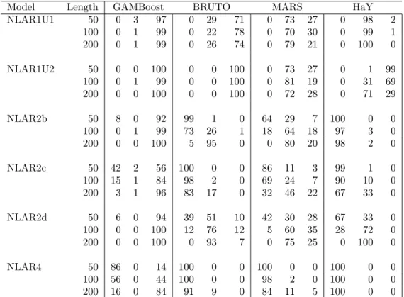
In this section we investigate the performance of boosting an additive model in Monte Carlo sim-ulations with six artificial, nonlinear, autoregressive time series. We compare the outcomes of boosting to the outcomes obtained through alternative nonparametric methods. Their performance is considered in two categories: in terms of lag-selection and goodness-of-fit. The dynamics of the simulated processes are shown in Table 1. NLAR1U1 and NLAR1U2 have one lag and were used by Huang and Yang (2004). Besides, there are three models with two lags: NLAR2b-NLAR2d. All but NLAR2c two-lag-models were originally used by Tschernig and Yang (2000), NLAR2c was used by Chen and Tsay (1993). The last model NLAR4 has four lags and was used by Shafik and Tutz (2009).
It this section we will juxtapose componentwise boosting of an additive model (GAMBoost), the method by Huang and Yang (2004), referred to with the acronym HaY, BRUTO and MARS.
3.1 Lag Selection 3 SIMULATION STUDY All models from Table 1 have been simulated 100 times with sizes 400 +N, the first 400 values discarded and N = p+T, with p = 10 pre-sample values andT = 50,100,200 in-sample observations. Such partitioning of the time series values is convenient in order to ensure same sample size ofT for each covariate at a given period and to simplify the notation. As psuggests, the maximal lag-length has been limited to ten. In the next section we compare the performance of the different procedures in terms of lag selection.
3.1 Lag Selection
The exposition in this section is inspired by Huang and Yang (2004). For each process we have an index sets, consisting of the numbers of the lags that have an effect, e.g., for NLAR2b,s={6,10}. Let ˆsbe a particular model estimation of s. The accuracy of the estimation is quantified by the following rule: ˆs is said to be correct if ˆs = s; ˆs is an overfit if ˆs ⊃ s; and ˆs is an underfit if (ˆs∩s) ⊂ s. Note that ˆs can be larger than s and still underfitting. In other words, underfit indicates that some significant variables have been erroneously omitted by the model, while overfit means inclusion of redundant variables in addition to the significant ones.
Table 2 gives a summary of the Monte Carlo simulations for all four fitting procedures. The first, second and third columns present the numbers of underfit, correct and overfit outcomes over 100 simulation runs. For example, MARS at NLAR2b withT = 100 has identified the index set 64 times correctly, has neglected at least one of the significant lags 18 times and has added more lags in 18 cases.
As Table 2 suggests, boosting an additive model is likely to overfit most of the time. This tendency is especially noticeable with fewer lags. Such performance of GAMBoost is in some sense expected. If in a single boosting step, some variable has been erroneously considered, that would be sufficient to add it to the estimated set ˆs. Although being a redundant variable, the corresponding function estimate can still be close to zero and therefore being interpreted as a random error. In the next section we explore whether such an influence is really considered as minimal or has a substantial counterproductive impact.
The non-boosting methods are more likely to underfit larger models. This is evident for NLAR2b and NLAR2c, and becomes especially noticeable for NLAR4. The last process is repeatedly un-derfitted by BRUTO, MARS and HaY, while GAMBoost encourages inclusion of more lags. We should, however, keep in mind that the mathematical properties for variable selection of boosting are still under construction (see Meinshausen and B¨uhlmann, 2010).
The performances of BRUTO, MARS and HaY for NLAR1U1, NLAR1U2 and NLAR2d pro-cesses are consistent with the results provided by Huang and Yang (2004). It should be noted that, in contrast to the cited paper, we have examined small to moderate sample sizes. Under these conditions, the auspicious approach HaY still demonstrates very good detection of true variables and steadily increases the frequency of correct fitting with increasing sample size. As reported in the Huang and Yang (2004), however, the cubic spline fitting faces some difficulties with NLAR2b. It performed poorly in our simulations too. In addition, HaY is the single model which underfitted 100% of the NLAR4 realizations.
One concern with the HaY method is that in high-dimensional models computations become prohibitive. Combining both forward and backward stages with maximum number ofd lags and number of candidate variables Smax, the forward stage requires PSi=1max(d−i+ 1) computations
and the backward stagePSmax
j=1 jcomputations. Particularly, whenSmax =p, wherepdenotes the
3.2 Estimation of Dynamics 3 SIMULATION STUDY
Model Length GAMBoost BRUTO MARS HaY
NLAR1U1 50 0 3 97 0 29 71 0 73 27 0 98 2 100 0 1 99 0 22 78 0 70 30 0 99 1 200 0 1 99 0 26 74 0 79 21 0 100 0 NLAR1U2 50 0 0 100 0 0 100 0 73 27 0 1 99 100 0 1 99 0 0 100 0 81 19 0 31 69 200 0 0 100 0 0 100 0 72 28 0 71 29 NLAR2b 50 8 0 92 99 1 0 64 29 7 100 0 0 100 0 1 99 73 26 1 18 64 18 97 3 0 200 0 0 100 5 95 0 0 80 20 98 2 0 NLAR2c 50 42 2 56 100 0 0 86 11 3 99 1 0 100 15 1 84 98 2 0 69 24 7 90 10 0 200 3 1 96 83 17 0 32 46 22 67 33 0 NLAR2d 50 6 0 94 39 51 10 42 30 28 67 33 0 100 0 0 100 12 76 12 5 60 35 28 72 0 200 0 0 100 0 93 7 0 75 25 0 100 0 NLAR4 50 86 0 14 100 0 0 100 0 0 100 0 0 100 56 0 44 100 0 0 98 2 0 100 0 0 200 16 0 84 91 9 0 84 11 5 100 0 0
Table 2: Simulation results for lag selection. The first, second and third columns in each setup show the number of underfit, correct and overfit outcomes over 100 simulation runs.
covariate contributes quadratically to the computational burden. For high dimensions that would be an essential issue.
MARS showed an overall good performance. It had the highest rate of significant hits with NLAR4 amongst the non-boosting methods. On the other hand, BRUTO showed a rather erratic behaviour by favouring processes like NLAR2b, NLAR2d and performing very poorly with the others.
3.2 Estimation of Dynamics
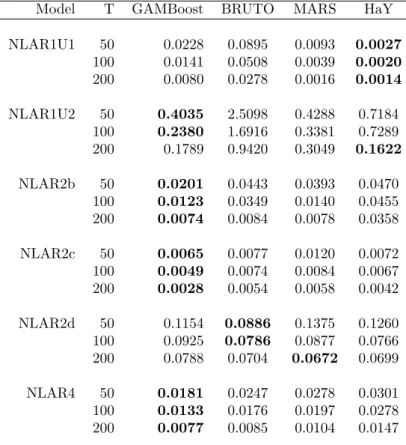
In simulations we can measure how precisely a fitting procedure reflects the true dynamics of a simulated process. In case of linear time series, a convenient measure is the Euclidian distance between the true parameter vector and the estimated one. When dealing with nonparametric models we need a more sophisticated accuracy measure for the discrepancy betweenfunctions. We consider the squared residuals between the true partial functions (or lag functions) centered to mean zero and the estimated functions.
3.2 Estimation of Dynamics 3 SIMULATION STUDY Model T GAMBoost BRUTO MARS HaY
NLAR1U1 50 0.0228 0.0895 0.0093 0.0027 100 0.0141 0.0508 0.0039 0.0020 200 0.0080 0.0278 0.0016 0.0014 NLAR1U2 50 0.4035 2.5098 0.4288 0.7184 100 0.2380 1.6916 0.3381 0.7289 200 0.1789 0.9420 0.3049 0.1622 NLAR2b 50 0.0201 0.0443 0.0393 0.0470 100 0.0123 0.0349 0.0140 0.0455 200 0.0074 0.0084 0.0078 0.0358 NLAR2c 50 0.0065 0.0077 0.0120 0.0072 100 0.0049 0.0074 0.0084 0.0067 200 0.0028 0.0054 0.0058 0.0042 NLAR2d 50 0.1154 0.0886 0.1375 0.1260 100 0.0925 0.0786 0.0877 0.0766 200 0.0788 0.0704 0.0672 0.0699 NLAR4 50 0.0181 0.0247 0.0278 0.0301 100 0.0133 0.0176 0.0197 0.0278 200 0.0077 0.0085 0.0104 0.0147
Table 3: Simulation results of the median MSPE of 100 simulation runs multiplied by 100. Boldface numbers indicate the best model performance for each setup.
value. Then the mean squared prediction error is MSPEk= 2001
200
X
i=1
[ ˜fk(zi)−fˆ˜k(zi)]2 (3.1)
where ˆ˜fk is the estimated counterpart of ˜fk. We choose thezi’s being evenly spaced between the
5th and 95th quantile of the empirical distribution ofyt−k. The accuracy measure is the average
of the individual MSPE’s
MSPE =
p
X
k=1
MSPEk. (3.2)
The results of the median MSPE across all 100 simulation runs are summarized in Table 3, where the rows give the simulated series and the columns represent the different modelling techniques. NLAR1U and NLAR1U2 yield the most parsimonious models. Their dynamics seems to be ex-plained very well by MARS, HaY and GAMBoost, while BRUTO performed very poorly. For
3.2 Estimation of Dynamics 3 SIMULATION STUDY ● ● ● ● ● ● ● ● ● ● ● ● ● ● ● ● ● ● ● ● −0.1 0.4 0.9 1.4 1.9 −0.68 −0.34 0.00 0.00 0.34 0.68 Lag 1 ●● ● ● ● ● ● ● ●● ● ● ● ● ● ● ● ● ● ● −0.1 0.4 0.9 1.4 1.9 −0.68 −0.34 0.00 0.00 0.34 0.68 Lag 2 ● ● ● ● ● ● ● ● ● ● ● ● ● ● ● ● ● ● ● ● −0.1 0.4 0.9 1.4 1.9 −0.68 −0.34 0.00 0.00 0.34 0.68 Lag 3 ● ● ● ● ● ● ● ● ● ● ● ● ● ● ● ● ● ● ● ● −0.1 0.4 0.9 1.4 1.9 −0.68 −0.34 0.00 0.00 0.34 0.68 Lag 4 ● ● ● ● ● ● ● ● ● ● ● ● ● ● ● ● ● ● ● ● −0.1 0.4 0.9 1.4 1.9 −0.68 −0.34 0.00 0.00 0.34 0.68 Lag 5 ● ● ● ● ● ● ● ● ● ● ● ● ● ● ● ● ● ● ● ● −0.1 0.4 0.9 1.4 1.9 −0.68 −0.34 0.00 0.00 0.34 0.68 Lag 6 ● ● ● ● ● ● ● ● ● ● ● ● ● ● ● ● ● ● ● ● −0.1 0.4 0.9 1.4 1.9 −0.68 −0.34 0.00 0.00 0.34 0.68 Lag 7 ● ● ● ● ● ● ● ● ● ● ● ● ● ● ● ● ● ● ● ● −0.1 0.4 0.9 1.4 1.9 −0.68 −0.34 0.00 0.00 0.34 0.68 Lag 8 ● ● ● ● ● ● ● ● ● ● ● ● ● ● ● ● ● ● ● ● −0.1 0.4 0.9 1.4 1.9 −0.68 −0.34 0.00 0.00 0.34 0.68 Lag 9 ● ● ● ● ● ● ● ● ● ● ● ● ● ● ● ● ● ● ● ● −0.1 0.4 0.9 1.4 1.9 −0.68 −0.34 0.00 0.00 0.34 0.68 Lag 10
Figure 1: Boosting estimations of the lag functions of NLAR1U2. True lag is 2 (circled line), estimated lags are depicted as solid lines. The functions are mean zero centered.
NLAR1U2, we notice that despite overfitting in sense of selected lags, boosting estimated the rel-evant function quite precisely, e.g.,T = 50,100. This suggests that the redundant functions were considered close to zero. It is reassuring to see the seemingly zero redundant lag estimations of NLAR1U2 in Figure 1.
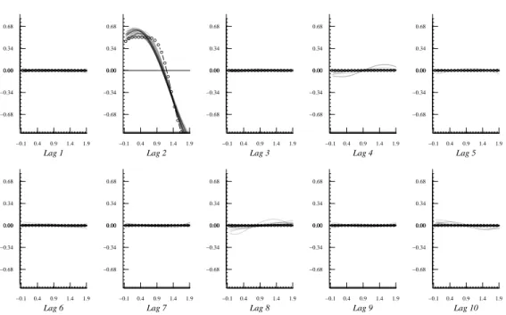
The literature on nonparametric regression for dependent data is relatively sparse, especially when related to boosting. Strong serial dependence might mislead the fitting procedure to produce erroneous transformations. For instance, this is evident for boosting of NLAR2c, shown Figure 2, where the second and the seventh lag were overfitted rather strongly.
With an increasing number of significant covariates both BRUTO and GAMBoost improved their performance. The boxplots shown in Figure 3 propose a visual confirmation of the last state-ment. They represent MSPE of each modelling strategy amongst the simulations repetitions. The exclusion of significant covariates by the non-boosting methods was, on balance, more counter-productive than the inclusion of redundant ones by boosting. GAMBoost showed, overall, strong estimation properties. Boosting was superior to its rivals in the larger model specifications and was evidently competitive even in the small ones. It is worth mentioning that boosting distinguished for the small sample sizes by larger margins. It showed good prediction quality when the information content of the data decreased, i.e., there was low signal-to-noise ratio.
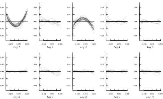
4 ECONOMIC FORECASTING WITH BOOSTING ● ● ● ● ● ● ●● ● ● ●●● ● ● ● ● ● ● ● −0.100 0.050 0.200 −0.08 −0.04 0.00 0.00 0.04 0.08 Lag 1 ● ● ● ● ● ● ● ● ● ● ● ● ● ● ● ● ● ● ● ● −0.100 0.050 0.200 −0.08 −0.04 0.00 0.00 0.04 0.08 Lag 2 ● ● ● ●● ●● ●● ● ● ●● ● ● ● ● ● ● ● −0.100 0.050 0.200 −0.08 −0.04 0.00 0.00 0.04 0.08 Lag 3 ● ● ● ● ● ● ● ● ● ● ● ● ● ● ● ● ● ● ● ● −0.100 0.050 0.200 −0.08 −0.04 0.00 0.00 0.04 0.08 Lag 4 ● ● ● ● ● ● ● ● ● ● ● ● ● ● ● ● ● ● ● ● −0.100 0.050 0.200 −0.08 −0.04 0.00 0.00 0.04 0.08 Lag 5 ● ● ● ● ● ● ● ● ● ● ● ● ● ● ● ● ● ● ● ● −0.100 0.050 0.200 −0.08 −0.04 0.00 0.00 0.04 0.08 Lag 6 ● ● ● ● ● ● ● ● ● ● ● ● ● ● ● ● ● ● ● ● −0.100 0.050 0.200 −0.08 −0.04 0.00 0.00 0.04 0.08 Lag 7 ● ● ● ● ● ● ● ● ● ● ● ● ● ● ● ● ● ● ● ● −0.100 0.050 0.200 −0.08 −0.04 0.00 0.00 0.04 0.08 Lag 8 ● ● ● ● ● ● ● ● ● ● ● ● ● ● ● ● ● ● ● ● −0.100 0.050 0.200 −0.08 −0.04 0.00 0.00 0.04 0.08 Lag 9 ● ● ● ● ● ● ● ● ● ● ● ● ● ● ● ● ● ● ● ● −0.100 0.050 0.200 −0.08 −0.04 0.00 0.00 0.04 0.08 Lag 10
Figure 2: Boosting estimations of the lag functions of NLAR2c. True lags are 1 and 3 (dashed lines), estimated lags are depicted as solid lines. The functions are mean zero centered.
4 Economic Forecasting with Boosting
In this section boosting, along with other parametric and nonparametric models, are applied to real data. The target variable is the German industrial production (IP) with 176 observations for the time period 1992:01 – 2006:08. In order to circumvent any structural breaks due to the reunification, the data before 1991 was omitted. Data from 1991 is not included either, because some of the exogenous variables used later, such as ZEW Economic Sentiment, FAZ Indicator, have only been available after 1992. The series was obtained from Deutsche Bundesbank1 and is
seasonally and workday adjusted. Along with the leading indicators in Section 4.3, the data was also used by Robinzonov and Wohlrabe (2010). The exact monthly growth rates are taken to eliminate non-stationarity which is
∆(IPt) =IPtIP−IPt−1 t−1 .
Forecasting of IP is frequently performed in practice. Contributions to the forecasting of German industrial production include H¨ufner and Schr¨oder (2002), Benner and Meier (2004), Dreger and Schumacher (2005) among others.
Historically, the focus in forecasting has been on low-dimensional univariate or multivariate models, all sharing the common linearity in the parameters. Recently additional studies exist that investigate the forecasting performance of nonlinear time series models, e.g., Clements, Franses
4 ECONOMIC FORECASTING WITH BOOSTING MSPE*100 0.01 0.02 0.03 0.04 0.05 0.06 BR UT O GAMBoost HaY MARS ● ● ● ● ●● ● ● ● ● ●● ● ● ●● ● ● ● ● ●● ● ● ●● ● ● ● NLAR2b, T = 050 BR UT O GAMBoost HaY MARS ● ● ● ● ● ● ● ● ● ● ● ● ● ● ● ●● NLAR2b, T = 100 BR UT O GAMBoost HaY MARS ● ● ● ● ● ● ● ● ●● ● ● ● ● ●● ● ●● ●● ●● ●● ●●● ●● ●●●●● ● ●● NLAR2b, T = 200 MSPE*100 0.5 1.0 1.5 2.0 2.5 3.0 BR UT O GAMBoost HaY MARS ● ● ● ● ● ●● ● ●● ● ● NLAR1U2, T = 050 BR UT O GAMBoost HaY MARS ● ● ● ● ● ● ●● ● ● ● ● ● ● ● ● NLAR1U2, T = 100 BR UT O GAMBoost HaY MARS ● ● ● ● ● ● ● ●● ● ● ● ●●● ● ● ● ● ●● ● ●●●● ● ● ● ●●● NLAR1U2, T = 200 MSPE*100 0.05 0.10 0.15 0.20 BR UT O GAMBoost HaY MARS ● ● ● ● ● ● ●●●●●● ● ● ● ● ● ● ● ● ● ● ● ●●●● ●●● ●●● NLAR1U1, T = 050 BR UT O GAMBoost HaY MARS ● ● ● ● ● ● ● ● ●● ● ● ● ● ● ● ●● ● ● ● ● ● ● ● ● ● ●● ● NLAR1U1, T = 100 BR UT O GAMBoost HaY MARS ● ● ● ● ● ● ● ● ● ●● ● ● ● ● ● ●●●● ● ● ● ●●● ● ● ● ● ● ● NLAR1U1, T = 200 MSPE*100 0.01 0.02 0.03 0.04 0.05 0.06 BR UT O GAMBoost HaY MARS ● ● ● ● ● ● ● ● ● ● ● ●● ●●●● ● ● ● ● ●● ● ●● ● ● ● ● NLAR4, T = 050 BR UT O GAMBoost HaY MARS ● ● ● ● ● ● ● ●● ● ● ● ●● ● ● ● ● ● ● ● ● ● NLAR4, T = 100 BR UT O GAMBoost HaY MARS ● ● ● ● ● ●● ●● ● ● NLAR4, T = 200 MSPE*100 0.05 0.10 0.15 0.20 0.25 BR UT O GAMBoost HaY MARS ● ● ● ● ● ● ● ● ● ● ● ● ● ● ●● ● ● ●●● ●●● ● ● ● ● ●● ● ● ● ● ● ●●● ●● ● ● NLAR2d, T = 050 BR UT O GAMBoost HaY MARS ● ● ● ● ●● ● ●● ● ● ● ● ● ● ● ● ●● ● ● ● ● ● ● ●●● ●●● NLAR2d, T = 100 BR UT O GAMBoost HaY MARS ● ● ● ● ● ●●● ●● ● ● ● ● ● ●● ● ● NLAR2d, T = 200 MSPE*100 0.005 0.010 0.015 0.020 0.025 BR UT O GAMBoost HaY MARS ● ● ● ● ● ● ● ● ● ● ● ●● ●● ● ● ● NLAR2c, T = 050 BR UT O GAMBoost HaY MARS ● ● ● ● ● ● ● ● ●● ● ● ●●●●● ●●● NLAR2c, T = 100 BR UT O GAMBoost HaY MARS ● ● ● ● ● ● ●● ● ● ●●● ●● ● NLAR2c, T = 200 Figure 3: Bo xplots of the Mon te-Carlo sim ulations.
4.1 Forecasting Principles 4 ECONOMIC FORECASTING WITH BOOSTING and Swanson (2004), Ter¨asvirta, van Dijk and Medeiros (2005), Claveria, Pons and Ramos (2007), Elliot and Timmermann (2008). The application of boosting by means ofeconomic forecasting is the major novelty in the present work.
4.1 Forecasting Principles
When a specific time series model is assumed and a set of observations is given, we want to predict. The given set of observations is called atraining set or aninformation set. The intention is to use the information inzt to predict the real outputsyt+h.
We use adirect forecasting strategy (e.g. Marcellino et al., 2006, Chevillon and Hendry, 2005). The idea is to use a horizon-specific estimation model, where response is the multiperiod ahead value. The approach differs from iterated forecasting. The question which method is preferable is an empirical one. The direct forecasting approach is surely a good choice under the presence of exogenous variables.
To evaluate accuracy of prediction we need to specify acost function. The choice of an accuracy measure is a major topic by itself. Hyndman and Koehler (2006) widely discussed and compared different measures of accuracy of times series forecasts. The references therein point the reader to different studies with often controversial conclusions about the “best” forecasting measure. Still, the literature being inconsistent, the MSE withstands the time proof and remains one of the most popular out-of-sample measures. Therefore, minimizing the quadraticexpected cost orloss
MSE = E (yt+h−yˆt+h|zt)2 (4.1)
is set as an objective. Expression (4.1) is known as the mean squared error, associated with the forecast ˆyt+h.
Further we are interested in obtaining estimations of multiple forecasting horizons. Therefore, we alter the information set consistently. One option is to fix the starting point of the information set and consecutively enlarge its size with new observations. This method is calledrecursivescheme for forecasting. We apply the direct type of forecasting with the above mentioned recursive scheme to all models in the remaining part of this paper.
4.2 Univariate Forecasting of Industrial Production
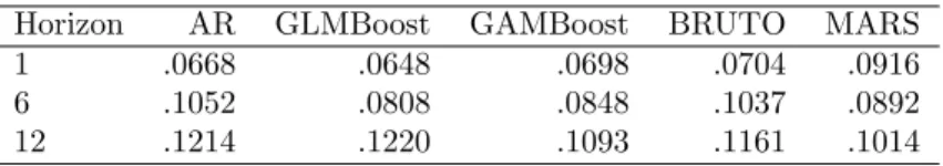
We apply GAMBoost, BRUTO, MARS and boosting with linear componentwise learner (referred to as GLMBoost, (2.10)) on the German industrial production. The univariate autoregressive model (AR) offers one of the simplest and most commonly used techniques for forecasting. It is easily applicable and therefore is often used as a benchmark model. The underlying assumption is that
Horizon AR GLMBoost GAMBoost BRUTO MARS
1 .0668 .0648 .0698 .0704 .0916
6 .1052 .0808 .0848 .1037 .0892
12 .1214 .1220 .1093 .1161 .1014
Table 4: Average squared forecast errors, multiplied by 103, of IP for 1, 6 and 12-periods ahead
forecasts of the monthly industrial production growth rates in Germany. The results are based on 20 forecasts.
4.2 Forecasting I 4 ECONOMIC FORECASTING WITH BOOSTING MSE x 1000 0.0 0.1 0.2 0.3 0.4 AR BR UTO GAMBoost GLMBoost MARS ● ● ● ● ● ● ● ● ● ● Horizon = 1 AR BR UTO GAMBoost GLMBoost MARS ● ● ● ● ● Horizon = 6 AR BR UTO GAMBoost GLMBoost MARS ● ● ● ● ● ● ● ● Horizon = 12
Figure 4: Boxplots of the average squared forecast errors (multiplied by 103) for 1, 6 and 12-periods
ahead forecasts of the univariate IP, based on 20 forecasts.
every alternative method should be at least as good as the autoregressive model in order to justify an increase in the model’s complexity.
The promising technique by Huang and Yang (2004) is omitted because Section 4.3 extends the available data set with exogenous variables, the so calledleading indicators, and determines how the additional information affects the performance of the models. The inclusion of exogenous variables and their lags rapidly increases the number of covariates, forming a classical high-dimensional modelling problem. In this context, the method of Huang and Yang (2004) is no longer applicable. For IP we have a total length of 176 observations. The initial information set is defined from the beginning 1992:01 until 2003:12, thus consisting of 144 observations. The maximal number of lags is limited to 12. At the first stage twelve forecasts are calculated, i.e., prognoses for 2004:1-2004:12. At the consecutive stage, the information set is enlarged with one observation and the corresponding horizon is re-estimated. We continue in this fashion until 2005:8 where the information set reaches its maximum. Thus, we compute twenty stages in total.
Table 4 gives a summary of the average squared forecast errors for IP, delivered by the differ-ent methods. Appardiffer-ently, in short term forecasting, the standard autoregressive model is quite a hard one to overcome. This simple, yet powerful, model is superior to BRUTO, MARS and GAMBoost for short-term forecasting. On the other hand, GLMBoost seems to be precise in short term forecasting. With increasing forecasting horizon, all alternative models provide better
fore-AR GLMBoost GAMBoost BRUTO MARS
Selected lags 1,2 1,2,3,6,7,8,11 1,2,3,5,6,7,9,10,11,12 1 1 Table 5: Selected variables when information set reached its maximum.
4.3 Forecasting II 4 ECONOMIC FORECASTING WITH BOOSTING
Indicator Provider Label
Ifo Business Climate Ifo Institute ifo
ZEW Economic Sentiment ZEW Institute zew
OECD Composite leading indicator for Germany OECD oecd
Early Bird Indicator Commerzbank com
FAZ Indicator FAZ Institute faz
Interest Rate: overnight IMF rovnght
Interest Rate: spread IMF rspread
Employment Growth Bundesbank emp
Factor Bundesbank factor
Table 6: Leading Indicators.
casts for the monthly German industrial production growth rates, compared to AR. Both boosting methods prove to be efficient in forecasting, especially the linear boosting in short and middle-term forecasting, where it offers the smallest prediction error in average. For the longest horizon GLM-Boost remains at least as good as AR, but performs relatively poorly in comparison to GAMGLM-Boost, BRUTO and MARS. Figure 4 depicts the differences between the models of the prediction squared errors.
In addition, Table 5 is considered to give an impression of the selected lags, chosen by the models. Selected lags may differ at the different stages, therefore we review the outcome at the stage where the information set reached its maximum (2005:08), being in this way the most representative. Both boosting techniques estimated quite large models, which is consistent with the results of the simulation study.
Based on the averaged errors in Table 4 and the given boxplots in Figure 4, it is rather challenging to announce a winning modelling strategy. It seems that the models assimilate the information, based solely on IP, efficiently. Therefore, in order to improve the models prediction quality we supply them with additional information in the following section.
4.3 Forecasting Industrial Production with Exogenous Variables
Forecasting of industrial production is based on the assumption that different leading indicators should relate significantly with the response, and therefore positively influence its prediction. There are many leading indicators, however, that “claim” such an appealing property. Usually, one indica-tor is taken and its forecasting potential is judged by a bivariate auindica-toregressive model, e.g., Dreger and Schumacher (2005) compared four indicators. The additional dimension does not necessarily improve the forecasting quality. On the contrary, in case of an “inappropriate” extra variable, it deteriorates the forecasting.
We collect the nine most commonly used indicators and investigate how they affect the forecast-ing. The aim is to investigate if it is still possible to obtain good forecasts, despite the presence of probably redundant variables. Table 6 contains a list of the nine frequently used leading indicators on forecasting German IP (see Appendix A for a detailed description of the indicators).
Since vector autoregressive analysis has evolved as a standard instrument in econometrics for analysing multivariate times series, we will consider nine bivariate models, each consisting of the IP and one leading indicator from Table 6 in its restricted (VARr) and unrestricted (VAR) form.
4.3 Forecasting II 4 ECONOMIC FORECASTING WITH BOOSTING
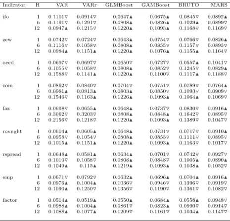
Indicator H VAR VARr GLMBoost GAMBoost BRUTO MARS
ifo 1 0.1101O 0.0914O 0.0647N 0.0675N 0.0845O 0.0892N 6 0.1191O 0.1291O 0.0808N 0.0826N 0.1029N 0.0899O 12 0.0947N 0.1215O 0.1220N 0.1093N 0.1168O 0.1169O zew 1 0.0742O 0.0724O 0.0643N 0.0754O 0.0766O 0.0826N 6 0.1116O 0.1058O 0.0808N 0.0855O 0.1157O 0.0893O 12 0.0984N 0.1151N 0.1220N 0.1076N 0.1155N 0.1164O oecd 1 0.0697O 0.0697O 0.0650O 0.0727O 0.0557N 0.1041O 6 0.1055O 0.1058O 0.0808N 0.0852O 0.1245O 0.0829N 12 0.1588O 0.1141N 0.1220N 0.1100O 0.1117N 0.1188O com 1 0.0862O 0.0840O 0.0704O 0.0751O 0.0789O 0.0764N 6 0.0981N 0.0813N 0.0803N 0.0850O 0.1093O 0.0909O 12 0.1546O 0.1163N 0.1226N 0.1093N 0.1064N 0.1069O faz 1 0.0698O 0.0655N 0.0648N 0.0737O 0.0830O 0.0916N 6 0.3062O 0.3203O 0.0808N 0.0848N 0.1642O 0.0895O 12 0.2156O 0.1218O 0.1220N 0.1093N 0.1389O 0.1047O rovnght 1 0.0604N 0.0605N 0.0648N 0.0731O 0.0717O 0.0910N 6 0.0958O 0.1054O 0.0808N 0.0853O 0.1111O 0.0895O 12 0.1015N 0.1151N 0.1220N 0.1093N 0.1163O 0.1017O rspread 1 0.0648N 0.0581N 0.0634N 0.0701O 0.0742O 0.0927O 6 0.1010O 0.1058O 0.0808N 0.0848O 0.1005N 0.0890N 12 0.1049N 0.115N 0.1219N 0.1093N 0.1038N 0.1052O emp 1 0.0671O 0.0792O 0.0632N 0.0696N 0.0704N 0.0916N 6 0.0976N 0.1004N 0.1036O 0.0946O 0.1396O 0.0919O 12 0.1090N 0.1250O 0.1356O 0.1190O 0.1361O 0.1082O factor 1 0.0514N 0.0519N 0.0550N 0.0684N 0.0558N 0.0948O 6 0.0988N 0.1004N 0.0861O 0.0823N 0.0990O 0.0914O 12 0.1088N 0.1077N 0.1209O 0.1161O 0.1034N 0.1147O
Table 7: Average squared forecast errors of the monthly industrial production growth rates in Germany, with one leading indicator as an exogenous variable. The results are based on 20 forecasts, multiplied by 103. The symbolNindicates forecast improve with respect to Table 4 andOindicates
decreased forecasting quality.
The restrictions are obtained via standard statisticalt-tests.
The inclusion of one exogenous variable means that we fit a model with 24 covariates, i.e., twelve for the IP and twelve for the exogenous variable. The forecasting outcome is documented in Table 7. Every triplet shows the average performance of the corresponding models, respectively for 1, 6 and 12-periods ahead forecasts. In addition, it is indicated whether the forecast quality increased or decreased with respect to the univariate forecasts in Table 5. Change of the forecasting quality for both VAR and VARr is compared to AR.
Figure 5 depicts the results from Table 7 together with the AR model in a more compact form in order to put an emphasize on the comparison. In the following a summary of the empirical results is given:
(a) The out-of-sample forecasting results from Table 7 suggest that both boosting techniques remain robust to the impact of the exogenous variables.
4.3 Forecasting II 4 ECONOMIC FORECASTING WITH BOOSTING to long-term forecasting (ifo, zew, oecd, faz and rovnght) GLMBoost did not consider the exogenous variable at all. This explains why these forecasts are identical to the univariate case in Table 4. Transferred to the indicators, this interpretation suggests that they have only a short term effect on IP. In one-period ahead forecasting the exogenous variable exerted negative impact on GLMBoost in two cases only (zew, com) and outperformed AR in all cases except for com. In general, substantial changes of GLMBoost, compared to the univariate forecasting, were not found. That implies that linear boosting considered IP with its own lags to a larger extent than the remaining covariates. As a result, it showed a very strong overall performance and outperformed most of the models for one and six-periods ahead forecasting. (b) The addition of exogenous variables changed the prediction power of GAMBoost, BRUTO and MARS with varying success. Most notably GAMBoost and MARS show good and stable performance for six and twelve-periods ahead forecasting. This is best seen by the illustration in Figure 5. BRUTO improved its short term forecasting performance with almost every variable (except for faz), but in general remained worse than AR. For longer horizons it showed a rather erratic behaviour.
(c) There are four leading indicators, which proved to have good forecasting quality in terms of bivariate linear autoregression. These are zew, faz, rspread and factor, which increased the forecasting precision of IP, compared to AR. Moreover, the restricted bivariate autoregressive model with factor and faz provided the best short-term forecasts, but was easily outperformed for longer horizons. It is evident also that the restricted model is superior to the unrestricted one in most of the cases.
(d) From a computational point of view, MARS and GLMBoost were the fastest procedures. Closely followed by BRUTO, VAR and VARr, they all perform comparably fast. Boosting with P-Spline weak learners was more computationally demanding.
In Table 8 lags are collected that were selected by boosting, BRUTO and MARS. The bivariate autoregressive models selected in most cases lag length of one (the results are not shown) which explains to some extent their relatively bad performance for longer forecasting horizons. It should be clearly stated that the selected lags by each method in Table 8 have resulted from a single, one-period ahead model with maximal information set. Therefore, they do not reflect the whole forecasting process and thus are not strictly related to the results, presented in Table 7. The intention is to gain a rather general impression of the selecting process.
It is reassuring to find support that GLMBoost considered IP with its own lags more heavily than the exogenous variables. In accordance with intuition this seems to be the most plausible forecasting strategy, since we forecast IP. In accordance to the forecasting results this was definitely the most successful one. Boosting with P-Spline weak learners seems to be very consistent in the selection of endogenous lags - the same subset of IP lags is almost always present. At the same time, it estimates the largest models. BRUTO is the single modelling strategy, which repeatedly considered more exogenous than endogenous lags. This partially explains its erratic forecasting behaviour, each time conducted by the new indicator.
In conclusion, for the monthly growth rates of the industrial production in Germany, we found evidence that boosting can be very competitive to the standard techniques. Particularly, least squares boosting predicts better than linear autoregressive models. The increased flexibility of the nonparametric models does not seem to pay-off in short term foreacasting, but manages to improve
5 CONCLUDING REMARKS MSE x 1000 0.06 0.08 0.10 0.12 0.14 0.16
com empfactor faz ifooecd rovnghtrspread zew ● ● ● ● ● ● ● ● ● Horizon = 1
com empfactor faz ifooecd rovnghtrspread zew ● ● ● ● ● ● ● ● ● Horizon = 6
com empfactor faz ifooecd rovnghtrspread zew 0.06 0.08 0.10 0.12 0.14 0.16 ● ● ● ● ● ● ● ● ● Horizon = 12 ● BRUTO GAMBoost GLMBoost MARS VAR VARr 0.06 0.08 0.10 0.12 0.14 0.16
com empfactor faz ifooecd rovnghtrspread
zew
Horizon = 1
com empfactor faz ifooecd rovnghtrspread
zew
Horizon = 6
com empfactor faz ifooecd rovnghtrspread zew 0.06 0.08 0.10 0.12 0.14 0.16 Horizon = 12 ● BRUTO GAMBoost GLMBoost MARS VAR VARr
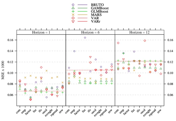
Figure 5: Average squared forecast errors of the monthly industrial production growth rates in Germany, with one leading indicator as an exogenous variable. Dashed red-line shows the value of the univariate autoregressive model. The results are based on 20 forecasts, multiplied by 103.
the prediction quality when the information content of the data decreases, i.e., low signal-to-noise ratio, which is observed in long-period ahead forecasting.
5 Concluding Remarks
In this paper several parametric and nonparametric modelling techniques for autoregressive time series are compared, with particular focus on boosting methods. By letting the covariates be lagged values of a time series, we have applied various strategies to identify relevant lags, estimates and forecasts. In Section 3 we proposed componentwise boosting of additive autoregressive model with P-Spline weak learners. Alternative modelling strategies were also applied on several nonlinear autoregressive time series. It is evidenced that boosting of high-order autoregressive time series can be very competitive in terms of dynamics estimation. Unlike regression analysis, however, the serial dependence in time series data might mislead the fitting procedure to produce erroneous
5 CONCLUDING REMARKS
Variable GLMBoost GAMBoost BRUTO MARS
IP 1,2,3,6,7,8 1,2,3,5,6,7,9,11,12 1,2 1 ifo 1 1,7,11 1,2,3,4,5,8,11,12 -IP 1,2,6,7,8 1,2,3,5,6,7,9,11,12 1,2 1 zew 1 1 1,2,3,5,6 1 IP 1,2,6,11,12 1,2,3,5,6,7,9,11,12 1,2 1 oecd 1 1,2,12 1,3,4,5,6,7,8,9,10 -IP 1,2,6,7,8,11,12 1,2,3,5,6,7,9,10,12 1,2 1 com 1,2,3 1,7,10 3,4,6,8 1 IP 1,2,3,6,7,8,11 1,2,3,6,7,9,10,11,12 1 1 faz - 7 1,2,3,4,5,6,7,8,9,10,11,12 -IP 1,2,3,6,7,8,11 1,2,3,6,7,9,10,11,12 1 1 rovnght - 7,10 2,3,4,5,6,7,8,9,10,11,12 -IP 1,2,3,6,7,8,11,12 1,2,3,6,7,9,10,11,12 1 1,3 rspread 1 1,4 1,2,3,4,7,10,11,12 1,4,7 IP 1,2,3,6,7,8,11,12 1,2,3,6,7,9,10,11,12 1 1 emp 1,4,6,9,12 1,8,9,11,12 - -IP 1,2,6,7,8,12 1,3,6,7,9,10,12 1,2,3,7 1,2 factor 3,4,11 1,2,3,5,7,8,11,12 3,7 1,7
Table 8: Selected lags of IP and of the exogenenous variable when the information set reached its maximum (horizonh= 1).
transformations. Care must be taken in using boosting algorithms in time series with strong serial correlation of the data. Further study on the use of boosting in time series context is needed to justify the general use of this procedure.
Another boosting strategy with parametric weak learners (GLMBoost) was included in order to perform a forecasting comparison, based on real world data in Section 4. The forecasting comparison was conducted over the monthly growth rates of the German industrial production (IP). Both boosting strategies managed to outperform the benchmark in macroeconomic forecasting, namely the linear autoregressive model. Moreover, it became clear that GLMBoost was the most successful strategy in terms of short and middle-term forecasting.
Additionally, the model was extended with different exogenous variables (leading indicators). We had nine indicators available and we included each of them separately, in addition to the target variable – the industrial production. Our intention was to investigate whether these variables do
5 CONCLUDING REMARKS indeed improve the forecasting quality of the industrial production and how boosting handles these high-dimensional models. Thus, having formed nine high-dimensional models, we forecasted again the monthly growth rates of IP. Linear bivariate autoregressive models were also considered as standard tools for forecasting. Our approach using componentwise linear and additive models in a function gradient descent algorithm improves upon likelihood based boosting applied to nonlinear autoregressive times series models (Shafik and Tutz, 2009) in two respects. First, more flexible regression functions can be estimated using our approach (linear effects, decompositions of linear and smooth effects or interaction effects (Kneib et al., 2009)). Second, further research established alternative characteristics of the response to be regressed on lags or exogenous variables, most importantly quantile regression approaches implemented via componentwise functional gradient descent (Fenske et al., 2009).
The variables’ impact on the forecasting quality had debatable success, since in many of the cases their inclusion worsened the forecasting performance, compared to the univariate case. GLMBoost, on the other hand, was almost immune to redundant variables by performing at least as good as in the univariate case. In one-period ahead forecasting, GAMBoost was affected by the additional variables rather strongly, which was counterproductive for its overall performance, when compared to the univariate case. The increased flexibility of GAMBoost was useful, however, in middle and long term forecasting, where the information content of the data is very low, i.e. it has low signal-to-noise ratio.
Another crucial topic for further development addresses the multivariate generalization of boost-ing. The first steps toward high dimensionality in the response were made by Lutz et al. (2007), who provided theoretical grounds and empirical evidence for its usability. Applying this approach would open new perspective for forecasting with boosting, based on iterative forecasts of multivariate models.
Computational Details
All data analyses presented in this paper have been carried out using the Rsystem for statistical computation (Team, 2009), version 2.9.2. There are several implementations of boosting techniques, available as add-on packages forR. Packagemboost(Hothorn et al., 2009) provides an implemen-tation for fitting generalized linear models, as well as additive gradient based boosting.
Our simulations were carried out withmboost. As weak learner we use P-Splines, provided by the functionbbs()and subsequently fitted by thegamboost() function.
We use 20 knots (knots = 20), we setM= 500 (mstop = 500) as an upper bound for boosting and set the degrees of freedom to 3.5, i.e. degree = 3.5. The optimal number of steps is evaluated via the corrected AIC criterion provided by theAIC() function. For all other options we use the default values.
Further on, we consider the method proposed by Huang and Yang (2004), which uses spline fitting with BIC. Their novel approach was manually implemented since it is currently not available as an extension package forRor in any other statistical software.
The implementation was carried out by the packagemgcv(Wood, 2006, 2009) with unpenalized cubic splines. The maximum number of candidate variables was equalled to the maximal number of lags.
An implementation of BRUTO can be found in packagemda(Hastie, Tibshirani, Leisch, Hornik and Ripley., 2009). The corresponding functionbruto() has a tuning parametercostwhich spec-ifies the cost per degree-of-freedom change. It was empirically investigated by Huang and Yang
5 CONCLUDING REMARKS (2004) that a value of log(n) provides much better results than the default value of two, wheren
indicates the sample size. Therefore, in our applicationcostwas set to log(n) too.
An implementation of MARS is available in package mda and the corresponding function is
mars(). It has a tuning parameter which charges a cost per basis function, denoted by penalty. This tuning parameter was also set to log(n).
The estimation of AR is carried out via thear()function in packagestatswith AIC criterion. The packagevars(Pfaff, 2008) offers “standard” tools in the context of purely vector autoregressive models. We use a modified version of its functionVARin order to consider direct forecasting. The corresponding information criterion is AIC.
A THE CHOICE OF LEADING INDICATORS
APPENDIX
A The Choice of Leading Indicators
In Section 4 nine leading indicators were chosen. These are summarized as follows.
The Ifo Business Climate Index is based on about 7,000 monthly survey responses of firms in manufacturing, construction, wholesaling and retailing. The firms are asked to give their assess-ments of the current business situation and their expectations for the next six months. The balance value of the current business situation is the difference of the percentages of the ”good” and respec-tively ”poor” responses, the balance value of the expectations is the difference of the percentages of the ”more favourable” and ”more unfavourable” responses. The business climate is a transformed mean of the balances of the business situation and the expectations. For further information see Goldrian (2007).
The ZEW Indicator of Economic Sentiment is published monthly. Up to 350 financial experts take part in the survey. The indicator reflects the difference between the share of analysts that are optimistic and the share of analysts that are pessimistic with regard to the expected economic development in Germany within six months (see H¨ufner and Schr¨oder, 2002).
The FAZ indicator (Frankfurter Allgemeine Zeitung) pools survey data and macroeconomic time series. It consists of the Ifo index (0.13), new orders in manufacturing industries (0.56), the real effective exchange rate of the Euro (0.06), the interest rate spread (0.08), the stock market index DAX (0.01), the number of job vacancies (0.05) and lagged industrial production (0.11). The Ifo index, orders in manufacturing and the number of job vacancies enter the indicator equation in levels, while the other variables are measured in first differences.
The Early Bird indicator, compiled by Commerzbank, also pools different time series and stresses the importance of international business cycles for the German economy. Its components are the real effective exchange rate of the Euro (0.35), the short-term real interest rate (0.4), defined as the difference between the short-term nominal rate and core inflation, and the purchasing manager index of U.S. manufactures (0.25).
The OECD composite leading indicator is delivered by using a modified version of the Phase-Average Trend method (PAT) developed by the US National Bureau of Economic Research (NBER). The indicator is compiled by combining de-trended component series in either their seasonally adjusted or raw form. The component series are selected based on various criteria such as economic significance, cyclical behaviour, data quality, timeliness and availability. For Germany the following time series are compiled: Orders inflow or demand: tendency (manufacturing) (% balance), Ifo Business climate indicator (manufacturing) (% balance), Spread of interest rates (% annual rate), Total new orders (manufacturing), Finished goods stocks: level (manufacturing) (% balance) and Export order books: level (manufacturing) (% balance).
Financial indicators, such as overnight interbank interest rate an interest spread, are used as possible predictors as well. Stock and Watson (2003) have conducted a thorough case study for different OECD countries by forecasting Gross Domestic Product (GDP), Inflation and Industrial production. The information on the growth of the employment in Germany has been taken from their paper.
Finally, a factor indicator obtained from a large data set from Germany, is included. The data set contains the German quarterly GDP and 111 monthly indicators from 1992 to 2006.2
REFERENCES REFERENCES
References
Benner, J. and Meier, C. (2004). Prognoseg¨ute alternativer Fr¨uhindikatoren f¨ur die Konjunktur in Deutschland,Jahrb¨ucher f¨ur National¨okonomie und Statistik224(6): 637–652.
B¨uhlmann, P. (2006). Boosting for high-dimensional linear models, The Annals of Statistics
34(2): 559–583.
B¨uhlmann, P. and Hothorn, T. (2007). Boosting algorithms: Regularization, prediction and model fitting,Statistical Science22(4): 477–505.
B¨uhlmann, P. and Yu, B. (2003). Boosting with thel2loss: Regression and classification, Journal
of the American Statistical Association98(462): 324–339.
Chen, R. and Tsay, R. (1993). Nonlinear additive ARX models,Journal of the American Statistical Association88(423): 955–967.
Chevillon, G. and Hendry, D. (2005). Non-parametric direct multi-step estimation for forecasting economic processes,International Journal of Forecasting21(2): 201–218.
Claveria, O., Pons, E. and Ramos, R. (2007). Business and consumer expectations and macroeco-nomic forecasts,International Journal of Forecasting23(1): 47–69.
Clements, M., Franses, P. and Swanson, N. (2004). Forecasting economic and financial time-series with non-linear models,International Journal of Forecasting20(2): 169–183.
Dreger, C. and Schumacher, C. (2005). Out-of-sample performance of leading indicators for the German business cycle. Single vs combined forecasts, Journal of Business Cycle Measurement and Analysis 2(1): 71–88.
Eilers, P. and Marx, B. (1996). Flexible smoothing with B-splines and penalties,Statistical Science
11(2): 89–102.
Elliot, G. and Timmermann, A. (2008). Economic forecasting, Journal of Economic Literature
66(1): 3–56.
Fenske, N., Kneib, T. and Hothorn, T. (2009). Identifying risk factors for severe childhood mal-nutrition by boosting additive quantile regression., Technical Report 52, Institut f¨ur Statistik, Ludwig-Maximilians-Universit¨at M¨unchen.
URL:http://epub.ub.uni-muenchen.de/10510/
Freund, Y. and Schapire, R. (1996). Experiments with a new boosting algorithm,Proceedings of the Thirteenth International Conference on Machine Learning, Morgan Kaufmann Publishers Inc., San Francisco, CA, pp. 148–156.
Friedman, J. (1991). Multivariate adaptive regression splines,The Annals of Statistics19(1): 1–67. Friedman, J. (2001). Greedy function approximation: A gradient boosting machine,The Annals of
Statistics29(5): 1189–1232.
REFERENCES REFERENCES Hastie, T. and Tibshirani, R. (1990). Generalized Additive Models, Chapman & Hall/CRC. Hastie, T., Tibshirani, R. and Friedman, J. (2001). The Elements of Statistical Learning: Data
Mining, Inference, and Prediction, Springer.
Hastie, T., Tibshirani, R. and Friedman, J. (2009). The Elements of Statistical Learning: Data Mining, Inference, and Prediction, 2nd edn, Springer.
Hastie, T., Tibshirani, R., Leisch, F., Hornik, K. and Ripley., B. D. (2009). mda: Mixture and Flexible Discriminant Analysis. R package version 0.3-4.
Hothorn, T., B¨uhlmann, P., Kneib, T. and Schmid, M. (2009). mboost: Model-Based Boosting, R package, version 1.0-7.
URL:http://CRAN.R-project.org/package=mboost
Huang, J. and Yang, L. (2004). Identification of non-linear additive autoregressive models,Journal of the Royal Statistical Society Series B(Statistical Methodology) 66(2): 463–477.
H¨ufner, F. and Schr¨oder, M. (2002). Prognosegehalt von ifo-Gesch¨aftserwartungen und ZEW-Konjunkturerwartungen: Ein ¨okonometrischer Vergleich, Jahrb¨ucher f¨ur National¨okonomie und Statistik222(3): 316–336.
Hurvich, C. M., Simonoff, J. S. and Tsai, C.-L. (1998). Smoothing parameter selection in nonpara-metric regression using an improved Akaike information criterion,Journal of the Royal Statistis-tical Society, Series B 60: 271–293.
Hyndman, R. and Koehler, A. (2006). Another look at measures of forecast accuracy,International Journal of Forecasting22(4): 679–688.
Kneib, T., Hothorn, T. and Tutz, G. (2009). Variable selection and model choice in geoadditive regression models, Biometrics65: 626–634.
Lewis, P. and Stevens, J. (1991). Nonlinear modeling of time series using multivariate adaptive regression splines (MARS).,Journal of the American Statistical Association86(416): 864–877. L¨utkepohl, H. (1991). Introduction to Multiple Time Series Analysis, Springer, Berlin.
L¨utkepohl, H. (2006). New Introduction to Multiple Time Series Analysis, Springer.
Lutz, R., Kalisch, M. and B¨uhlmann, P. (2007). Robustifiedl2boosting,Technical report, Seminar
fur Statistik ETH Zurich.
Marcellino, M. and Schumacher, C. (2007). Factor nowcasting of German GDP with ragged-edge data. A model comparison using MIDAS projections, Technical report, Bundesbank Discussion Paper, Series 1, 34/2007.
Marcellino, M., Stock, J. and Watson, M. (2006). A comparison of direct and iterated multistep AR methods for forecasting macroeconomic time series,Journal of Econometrics135(1-2): 499–526. Meinshausen, N. and B¨uhlmann, P. (2010). Stability selection, Journal of the Royal Statistical
REFERENCES REFERENCES Pfaff, B. (2008). VAR, SVAR and SVEC models: Implementation within R package vars,Journal
of Statistical Software 27(4).
URL:http://www.jstatsoft.org/v27/i04/
Robinzonov, N. and Wohlrabe, K. (2010). Freedom of choice in macroeconomic forecasting,CESifo Economic Studies 56(1).
Schmid, M. and Hothorn, T. (2008). Boosting additive models using component-wise P-splines, Computational Statistics & Data Analysis53(2): 298–311.
Shafik, N. and Tutz, G. (2009). Boosting nonlinear additive autoregressive time series, Computa-tional Statistics & Data Analysis 53(7): 2453–2464.
Stock, J. and Watson, M. (2003). Forecasting output and inflation: The role of asset prices,Journal of Economic Literature41(3): 788–829.
Team, R. D. C. (2009). R: A Language and Environment for Statistical Computing, R Foundation for Statistical Computing, Vienna, Austria. ISBN 3-900051-07-0.
URL:http://www.R-project.org
Ter¨asvirta, T., van Dijk, D. and Medeiros, M. (2005). Linear models, smooth transition autore-gressions, and neural networks for forecasting macroeconomic time series: A reexamination, International Journal of Forecasting21(4): 755–774.
Tschernig, R. and Yang, L. (2000). Nonparametric lag selection for time series, Journal of Time Series Analysis 21(4): 457–487.
Wood, S. (2006). Generalized Additive Models: An Introduction with R, Chapman & Hall/CRC. Wood, S. (2009). mgcv: GAMs with GCV smoothness estimation and GAMMs by REML/PQL, R