Lawrence Berkeley National Laboratory
Recent Work
Title
Definitions, methods, and applications in interpretable machine learning.
Permalink
https://escholarship.org/uc/item/13x9q01k
Journal
Proceedings of the National Academy of Sciences of the United States of America,
116(44)
ISSN
0027-8424
Authors
Murdoch, W James
Singh, Chandan
Kumbier, Karl
et al.
Publication Date
2019-10-16
DOI
10.1073/pnas.1900654116
Peer reviewed
STATISTICS
Definitions, methods, and applications in interpretable
machine learning
W. James Murdocha,1, Chandan Singhb,1, Karl Kumbiera,2, Reza Abbasi-Aslb,c,d,2, and Bin Yua,b,3
aStatistics Department, University of California, Berkeley, CA 94720;bElectrical Engineering and Computer Science Department, University of California,
Berkeley, CA 94720;cDepartment of Neurology, University of California, San Francisco, CA 94158; anddAllen Institute for Brain Science, Seattle, WA 98109
Contributed by Bin Yu, July 1, 2019 (sent for review January 16, 2019; reviewed by Rich Caruana and Giles Hooker)
Machine-learning models have demonstrated great success in learning complex patterns that enable them to make predic-tions about unobserved data. In addition to using models for prediction, the ability to interpret what a model has learned is receiving an increasing amount of attention. However, this increased focus has led to considerable confusion about the notion of interpretability. In particular, it is unclear how the wide array of proposed interpretation methods are related and what common concepts can be used to evaluate them. We aim to address these concerns by defining interpretability in the context of machine learning and introducing the predictive, descriptive, relevant (PDR) framework for discussing interpretations. The PDR framework provides 3 overarching desiderata for evaluation: predictive accuracy, descriptive accuracy, and relevancy, with rel-evancy judged relative to a human audience. Moreover, to help manage the deluge of interpretation methods, we introduce a categorization of existing techniques into model-based and post hoc categories, with subgroups including sparsity, modularity, and simulatability. To demonstrate how practitioners can use the PDR framework to evaluate and understand interpretations, we provide numerous real-world examples. These examples high-light the often underappreciated role played by human audiences in discussions of interpretability. Finally, based on our frame-work, we discuss limitations of existing methods and directions for future work. We hope that this work will provide a com-mon vocabulary that will make it easier for both practitioners and researchers to discuss and choose from the full range of interpretation methods.
interpretability|machine learning|explainability|relevancy
M
achine learning (ML) has recently received considerable attention for its ability to accurately predict a wide variety of complex phenomena. However, there is a growing realization that, in addition to predictions, ML models are capable of pro-ducing knowledge about domain relationships contained in data, often referred to as interpretations. These interpretations have found uses in their own right, e.g., medicine (1), policymaking (2), and science (3, 4), as well as in auditing the predictions them-selves in response to issues such as regulatory pressure (5) and fairness (6). In these domains, interpretations have been shown to help with evaluating a learned model, providing information to repair a model (if needed), and building trust with domain experts (7).In the absence of a well-formed definition of interpretability, a broad range of methods with a correspondingly broad range of outputs (e.g., visualizations, natural language, mathematical equations) have been labeled as interpretation. This has led to considerable confusion about the notion of interpretability. In particular, it is unclear what it means to interpret something, what common threads exist among disparate methods, and how to select an interpretation method for a particular problem/ audience.
In this paper, we attempt to address these concerns. To do so, we first define interpretability in the context of machine learning and place it within a generic data science life cycle. This allows us to distinguish between 2 main classes of interpretation methods:
model based∗ and post hoc. We then introduce the predictive, descriptive, relevant (PDR) framework, consisting of 3 desider-ata for evaluating and constructing interpretations: predictive accuracy, descriptive accuracy, and relevancy, where relevancy is judged by a human audience. Using these terms, we categorize a broad range of existing methods, all grounded in real-world examples.† In doing so, we provide a common vocabulary for researchers and practitioners to use in evaluating and selecting interpretation methods. We then show how our work enables a clearer discussion of open problems for future research.
1. Defining Interpretable Machine Learning
On its own, interpretability is a broad, poorly defined concept. Taken to its full generality, to interpret data means to extract information (of some form) from them. The set of methods falling under this umbrella spans everything from designing an initial experiment to visualizing final results. In this overly gen-eral form, interpretability is not substantially different from the established concepts of data science and applied statistics.
Instead of general interpretability, we focus on the use of interpretations to produce insight from ML models as part of the larger data–science life cycle. We define interpretable machine learning as the extraction of relevant knowledge from
Significance
The recent surge in interpretability research has led to con-fusion on numerous fronts. In particular, it is unclear what it means to be interpretable and how to select, evaluate, or even discuss methods for producing interpretations of machine-learning models. We aim to clarify these concerns by defining interpretable machine learning and constructing a unifying framework for existing methods which highlights the underappreciated role played by human audiences. Within this framework, methods are organized into 2 classes: model based and post hoc. To provide guidance in selecting and evaluating interpretation methods, we introduce 3 desiderata: predictive accuracy, descriptive accuracy, and relevancy. Using our framework, we review existing work, grounded in real-world studies which exemplify our desiderata, and suggest directions for future work.
Author contributions: W.J.M., C.S., K.K., R.A.-A., and B.Y. designed research; W.J.M., C.S.,
K.K., and R.A.-A., performed research; and W.J.M. and C.S. wrote the paper.y
Reviewers: R.C., Microsoft Research; and G.H., Cornell University.y
The authors declare no competing interest.y
Published under thePNAS license.y
1W.J.M. and C.S. contributed equally to this work.y
2K.K. and R.A.-A. contributed equally to this work.y
3To whom correspondence may be addressed. Email: [email protected].y
This article contains supporting information online atwww.pnas.org/lookup/suppl/doi:10.
1073/pnas.1900654116/-/DCSupplemental.y
First published October 16, 2019.
*For clarity, throughout this paper we use the term “model” to refer to both
machine-learning models and algorithms.
†Examples were selected through a nonexhaustive search of related work.
a machine-learning model concerning relationships either con-tained in data or learned by the model. Here, we view knowledge as being relevant if it provides insight for a particular audience into a chosen problem. These insights are often used to guide communication, actions, and discovery. They can be produced in formats such as visualizations, natural language, or mathe-matical equations, depending on the context and audience. For instance, a doctor who must diagnose a single patient will want qualitatively different information than an engineer determining whether an image classifier is discriminating by race. What we define as interpretable ML is sometimes referred to as explain-able ML, intelligible ML, or transparent ML. We include these headings under our definition.
2. Background
Interpretability is a quickly growing field in machine learning, and there have been multiple works examining various aspects of interpretations (sometimes under the heading, explainable AI). One line of work focuses on providing an overview of dif-ferent interpretation methods with a strong emphasis on post hoc interpretations of deep learning models (8, 9), sometimes pointing out similarities between various methods (10, 11). Other work has focused on the narrower problem of evaluating inter-pretations (12, 13) and what properties they should satisfy (14). These previous works touch on different subsets of interpretabil-ity, but do not address interpretable machine learning as a whole, and give limited guidance on how interpretability can actually be used in data–science life cycles. We aim to do so by provid-ing a framework and vocabulary to fully capture interpretable machine learning, its benefits, and its applications to concrete data problems.
Interpretability also plays a role in other research areas. For example, interpretability is a major topic when considering bias and fairness in ML models (15–17). In psychology, the general notions of interpretability and explanations have been studied at a more abstract level (18, 19), providing relevant conceptual per-spectives. Additionally, we comment on 2 related areas that are distinct but closely related to interpretability: causal inference and stability.
Causal Inference. Causal inference (20) is a subject from statis-tics which is related, but distinct, from interpretable machine learning. According to a prevalent view, causal inference meth-ods focus solely on extracting causal relationships from data, i.e., statements that altering one variable will cause a change in another. In contrast, interpretable ML, and most other sta-tistical techniques, is used to describe general relationships. Whether or not these relationships are causal cannot be verified through interpretable ML techniques, as they are not designed to distinguish between causal and noncausal effects.
In some instances, researchers use both interpretable machine learning and causal inference in a single analysis (21). One form of this is where the noncausal relationships extracted by inter-pretable ML are used to suggest potential causal relationships. These relationships can then be further analyzed using causal inference methods and fully validated through experimental studies.
Stability. Stability, as a generalization of robustness in statistics, is a concept that applies throughout the entire data–science life cycle, including interpretable ML. The stability principle requires that each step in the life cycle is stable with respect to appropri-ate perturbations, such as small changes in the model or data. Recently, stability has been shown to be important in applied statistical problems, for example when trying to make conclu-sions about a scientific problem (22) and in more general settings (23). Stability can be helpful in evaluating interpretation meth-ods and is a prerequisite for trustworthy interpretations. That
is, one should not interpret parts of a model which are not sta-ble to appropriate perturbations to the model and data. This is demonstrated through examples in the text (21, 24, 25).
3. Interpretation in the Data–Science Life Cycle
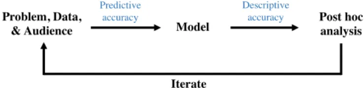
Before discussing interpretation methods, we first place the process of interpretable ML within the broader data–science life cycle. Fig. 1 presents a deliberately general description of this process, intended to capture most data-science problems. What is generally referred to as interpretation largely occurs in the modeling and post hoc analysis stages, with the prob-lem, data, and audience providing the context required to choose appropriate methods.
Problem, Data, and Audience. At the beginning of the cycle, a data–science practitioner defines a domain problem that the practitioner wishes to understand using data. This problem can take many forms. In a scientific setting, the practitioner may be interested in relationships contained in the data, such as how brain cells in a particular area of the visual system relate to visual stimuli (26). In industrial settings, the problem often concerns the predictive performance or other qualities of a model, such as how to assign credit scores with high accuracy (27) or do so fairly with respect to gender and race (17). The nature of the prob-lem plays a role in interpretability, as the relevant context and audience are essential in determining what methods to use.
After choosing a domain problem, the practitioner collects data to study it. Aspects of the data-collection process can affect the interpretation pipeline. Notably, biases in the data (i.e., mismatches between the collected data and the population of interest) will manifest themselves in the model, restricting one’s ability to generalize interpretations generated from the data to the population of interest.
Model.Based on the chosen problem and collected data, the practitioner then constructs a predictive model. At this stage, the practitioner processes, cleans, and visualizes data; extracts features; selects a model (or several models); and fits it. Inter-pretability considerations often come into play in this step related to the choice between simpler, easier to interpret mod-els and more complex, black-box modmod-els, which may fit the data better. The model’s ability to fit the data is measured through predictive accuracy.
Post Hoc Analysis. Having fitted a model (or models), the practi-tioner then analyzes it for answers to the original question. The process of analyzing the model often involves using interpretabil-ity methods to extract various (stable) forms of information from the model. The extracted information can then be analyzed and displayed using standard data analysis methods, such as scat-ter plots and histograms. The ability of the inscat-terpretations to properly describe what the model has learned is denoted by descriptive accuracy.
Iterate. If sufficient answers are uncovered after the post hoc analysis stage, the practitioner finishes. Otherwise, the
Fig. 1. Overview of different stages (black text) in a data–science life cycle where interpretability is important. Main stages are discussed inSection 3
STATISTICS practitioner updates something in the chain (problem, data,
and/or model) and the iterate (28). Note that the practitioner can terminate the loop at any stage, depending on the context of the problem.
Interpretation Methods within the PDR Framework. In the frame-work described above, our definition of interpretable ML focuses on methods in either the modeling or post hoc analysis stages. We call interpretability in the modeling stage model-based inter-pretability (Section 5). This part of interinter-pretability is focused upon the construction of models that readily provide insight into the relationships they have learned. To provide this insight, model-based interpretability techniques must generally use sim-pler models, which can result in lower predictive accuracy. Con-sequently, model-based interpretability is best used when the underlying relationship is sufficiently simple that model-based techniques can achieve reasonable predictive accuracy or when predictive accuracy is not a concern.
We call interpretability in the post hoc analysis stage post hoc interpretability (Section 6). In contrast to model-based inter-pretability, which alters the model to allow for interpretation, post hoc interpretation methods take a trained model as input and extract information about what relationships the model has learned. They are most helpful when the data are especially com-plex, and practitioners need to train a black-box model to achieve reasonable predictive accuracy.
After discussing desiderata for interpretation methods, we investigate these 2 forms of interpretations in detail and discuss associated methods.
4. The PDR Desiderata for Interpretations
In general, it is unclear how to select and evaluate interpreta-tion methods for a particular problem and audience. To help guide this process, we introduce the PDR framework, consisting of 3 desiderata that should be used to select interpretation meth-ods for a particular problem: predictive accuracy, descriptive accuracy, and relevancy.
A. Accuracy. The information produced by an interpretation method should be faithful to the underlying process the practi-tioner is trying to understand. In the context of ML, there are 2 areas where errors can arise: when approximating the underlying data relationships with a model (predictive accuracy) and when approximating what the model has learned using an interpreta-tion method (descriptive accuracy). For an interpretainterpreta-tion to be trustworthy, one should try to maximize both of the accuracies. In cases where either accuracy is not very high, the resulting inter-pretations may still be useful. However, it is especially important to check their trustworthiness through external validation, such as running an additional experiment.
A.1. Predictive accuracy. The first source of error occurs during the model stage, when an ML model is constructed. If the model learns a poor approximation of the underlying relationships in the data, any information extracted from the model is unlikely to be accurate. Evaluating the quality of a model’s fit has been well studied in standard supervised ML frameworks, through mea-sures such as test-set accuracy. In the context of interpretation, we describe this error as predictive accuracy.
Note that in problems involving interpretability, one must appropriately measure predictive accuracy. In particular, the data used to check for predictive accuracy must resemble the population of interest. For instance, evaluating on patients from one hospital may not generalize to others. Moreover, problems often require a notion of predictive accuracy that goes beyond just average accuracy. The distribution of predictions matters. For instance, it could be problematic if the prediction error is much higher for a particular class. Finally, the predictive accu-racy should be stable with respect to reasonable data and model
perturbations. One should not trust interpretations from a model which changes dramatically when trained on a slightly smaller subset of the data.
A.2. Descriptive accuracy. The second source of error occurs dur-ing the post hoc analysis stage, when interpretation methods are used to analyze a fitted model. Oftentimes, interpretations pro-vide an imperfect representation of the relationships learned by a model. This is especially challenging for complex black-box mod-els such as neural networks, which store nonlinear relationships between variables in nonobvious forms.
Definition: We define descriptive accuracy, in the context of interpretation, as the degree to which an interpretation method objectively captures the relationships learned by machine-learning models.
A.3. A common conflict: predictive vs. descriptive accuracy. In selecting what model to use, practitioners are sometimes faced with a trade-off between predictive and descriptive accuracy. On the one hand, the simplicity of model-based interpreta-tion methods yields consistently high descriptive accuracy, but can sometimes result in lower predictive accuracy on complex datasets. On the other hand, in complex settings such as image analysis, complicated models can provide high predictive accu-racy, but are harder to analyze, resulting in a lower descriptive accuracy.
B. Relevancy. When selecting an interpretation method, it is not enough for the method to have high accuracy—the extracted information must also be relevant. For example, in the context of genomics, a patient, doctor, biologist, and statistician may each want different (yet consistent) interpretations from the same model. The context provided by the problem and data stages in Fig. 1 guides what kinds of relationships a practitioner is inter-ested in learning about and by extension the methods that should be used.
Definition: We define an interpretation to be relevant if it provides insight for a particular audience into a chosen domain problem.
Relevancy often plays a key role in determining the trade-off between predictive and descriptive accuracy. Depending on the context of the problem at hand, a practitioner may choose to focus on one over the other. For instance, when interpretability is used to audit a model’s predictions, such as to enforce fair-ness, descriptive accuracy can be more important. In contrast, interpretability can also be used solely as a tool to increase the predictive accuracy of a model, for instance, through improved feature engineering.
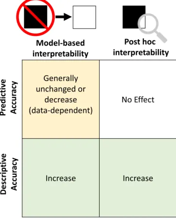
Having outlined the main desiderata for interpretation meth-ods, we now discuss how they link to interpretation in the modeling and post hoc analysis stages in the data–science life cycle. Fig. 2 draws parallels between our desiderata for interpre-tation techniques introduced inSection 4and our categorization of methods inSections 5and6. In particular, both post hoc and model-based methods aim to increase descriptive accuracy, but only the model-based method affects the predictive accuracy. Not shown is relevancy, which determines what type of output is helpful for a particular problem and audience.
5. Model-Based Interpretability
We now discuss how interpretability considerations come into play in the modeling stage of the data–science life cycle (Fig. 1). At this stage, the practitioner constructs an ML model from the collected data. We define model-based interpretability as the construction of models that readily provide insight into the relationships they have learned. Different model-based inter-pretability methods provide different ways of increasing descrip-tive accuracy by constructing models which are easier to under-stand, sometimes resulting in lower predictive accuracy. The main challenge of model-based interpretability is to come up
Fig. 2. Impact of interpretability methods on descriptive and predictive accuracies. Model-based interpretability (Section 5) involves using a sim-pler model to fit the data which can negatively affect predictive accuracy, but yields higher descriptive accuracy. Post hoc interpretability (Section 6) involves using methods to extract information from a trained model (with no effect on predictive accuracy). These correspond to the model and post hoc stages in Fig. 1.
with models that are simple enough to be easily understood by the audience, while maintaining high predictive accuracy.
In selecting a model to solve a domain problem, the practi-tioner must consider the entirety of the PDR framework. The first desideratum to consider is predictive accuracy. If the con-structed model does not accurately represent the underlying problem, any subsequent analysis will be suspect (29, 30). Sec-ond, the main purpose of model-based interpretation methods is to increase descriptive accuracy. Finally, the relevancy of a model’s output must be considered and is determined by the con-text of the problem, data, and audience. We now discuss some common types of model-based interpretability methods.
A. Sparsity. When the practitioner believes that the underlying relationship in question is based upon a sparse set of signals, the practitioner can impose sparsity on the model by limiting the number of nonzero parameters. In this section, we focus on lin-ear models, but sparsity can be helpful more generally. When the number of nonzero parameters is sufficiently small, a practitioner can interpret the variables corresponding to those parameters as being meaningfully related to the outcome in question and can also interpret the magnitude and direction of the parameters. However, before one can interpret a sparse parameter set, one should check for stability of the parameters. For example, if the signs/magnitudes of parameters or the predictions change due to small perturbations in the dataset, the coefficients should not be interpreted (31).
When the practitioner is able to correctly incorporate sparsity into the model, it can improve all 3 interpretation desiderata. By
reducing the number of parameters to analyze, sparse models can be easier to understand, yielding higher descriptive accu-racy. Moreover, incorporating prior information in the form of sparsity into a sparse problem can help a model achieve higher predictive accuracy and yield more relevant insights. Note that incorporating sparsity can often be quite difficult, as it requires understanding the data-specific structure of the sparsity and how it can be modeled.
Methods for obtaining sparsity often utilize a penalty on a loss function, such as LASSO (32) and sparse coding (33), or on model selection criteria such as AIC or BIC (34, 35). Many search-based methods have been developed to find sparse solutions. These methods search through the space of nonzero coefficients using classical subset-selection methods [e.g., orthog-onal matching pursuit (36)]. Model sparsity is often useful for high-dimensional problems, where the goal is to identify key fea-tures for further analysis. For instance, sparsity penalties have been incorporated into random forests to identify a sparse subset of important features (37).
In the following example from genomics, sparsity is used to increase the relevancy of an interpretation by reducing the number of potential interactions to a manageable level.
Example (Ex): Identifying interactions among regulatory fac-tors or biomolecules is an important question in genomics. Typical genomic datasets include thousands or even millions of features, many of which are active in specific cellular or developmental contexts. The massive scale of such datasets makes interpretation a considerable challenge. Sparsity penalties are frequently used to make the data manageable for statisti-cians and their collaborating biologists to discuss and identify promising candidates for further experiments.
For instance, one recent study (24) uses a biclustering approach based on sparse canonical correlation analysis (SCCA) to identify interactions among genomic expression features in Drosophila melanogaster (fruit flies) and Caenorhabditis ele-gans(roundworms). Sparsity penalties enable key interactions among features to be summarized in heatmaps which contain few enough variables for a human to analyze. The authors of this study also perform stability analysis, finding their model to be robust to different initializations and perturbations to hyperparameters.
B. Simulatability.A model is said to be simulatable if a human (for whom the interpretation is intended) is able to internally simulate and reason about its entire decision-making process (i.e., how a trained model produces an output for an arbitrary input). This is a very strong constraint to place on a model and can generally be done only when the number of features is low and the underlying relationship is simple. Decision trees (38) are often cited as a simulatable model, due to their hierarchical decision-making process. Another example is lists of rules (39, 40), which can easily be simulated. However, it is important to note that these models cease to be simulatable when they become large. In particular, as the complexity of the model increases (number of nodes in a decision tree or the number of rules in a list), it becomes increasingly difficult for a human to internally simulate.
Due to their simplicity, simulatable models have very high descriptive accuracy. When they can also provide reasonable predictive accuracy, they can be very effective. In the following example, a simulatable model is able to produce high predictive accuracy, while maintaining the high levels of descriptive accu-racy and relevancy normally attained by small-scale rules-based models.
Ex: In medical practice, when a patient has been diagnosed with atrial fibrillation, caregivers often want to predict the risk that the particular patient will have a stroke in the next year. Given the potential ramifications of medical decisions, it
STATISTICS is important that these predictions are not only accurate, but
interpretable to both the caregivers and patients.
To make the prediction, ref. 40 uses data from 12,586 patients detailing their age, gender, history of drugs and conditions, and whether they had a stroke within 1 y of diagnosis. To construct a model that has high predictive and descriptive accuracy, ref. 40 introduces a method for learning lists of if–then rules that are predictive of 1-y stroke risk. The resulting classifier, displayed in SI Appendix, Fig. S1, requires only 7 if–then statements to achieve competitive accuracy and is easy for even nontechnical practitioners to quickly understand.
Although this model is able to achieve high predictive and descriptive accuracy, it is important to note that the lack of stability in these types of models can limit their uses. If the practitioner’s intent is to simply understand a model that is ulti-mately used for predictions, these types of models can be very effective. However, if the practitioner wants to produce knowl-edge about the underlying dataset, the fact that the learned rules can change significantly when the model is retrained limits their generalizability.
C. Modularity. We define an ML model to be modular if a meaningful portion(s) of its prediction-making process can be interpreted independently. A wide array of models satisfies mod-ularity to different degrees. Generalized additive models (41) force the relationship between variables in the model to be addi-tive. In deep learning, specific methods such as attention (42) and modular network architectures (43) provide limited insight into a network’s inner workings. Probabilistic models can enforce modularity by specifying a conditional independence structure which makes it easier to reason about different parts of a model independently (44).
The following example uses modularity to produce relevant interpretations for use in diagnosing biases in training data.
Ex: When prioritizing patient care for patients with pneumo-nia in a hospital, one possible method is to predict the likelihood of death within 60 d and focus on the patients with a higher mor-tality risk. Given the potential life and death consequences, being able to explain the reasons for hospitalizing a patient or not is very important.
A recent study (7) uses a dataset of 14,199 patients with pneu-monia, with 46 features including demographics (e.g., age and gender), simple physical measurements (e.g., heart rate, blood pressure), and laboratory tests (e.g., white blood cell count, blood urea nitrogen). To predict mortality risk, the researchers use a generalized additive model with pairwise interactions, dis-played below. The univariate and pairwise terms (fj(xj) and
fij(xi,xj)) can be individually interpreted in the form of curves
and heatmaps, respectively:
g(E[y]) =β0+ X j fj(xj) + X i6=j fij(xi,xj). [1]
By inspecting the individual modules, the researchers found a number of counterintuitive properties of their model. For instance, the fitted model learned that having asthma is asso-ciated with a lower risk of dying from pneumonia. In reality, the opposite is true—patients with asthma are known to have a higher risk of death from pneumonia. Because of this, in the collected data all patients with asthma received aggressive care, which was fortunately effective at reducing their risk of mortality relative to the general population.
In this instance, if the model were used without having been interpreted, pneumonia patients with asthma would have been deprioritized for hospitalization. Consequently, the use of ML would increase their likelihood of dying. Fortunately, the use of an interpretable model enabled the researchers to identify and
correct errors like this one, better ensuring that the model could be trusted in the real world.
D. Domain-Based Feature Engineering.While the type of model is important in producing a useful interpretation, so are the features that are used as inputs to the model. Having more informative features makes the relationship that needs to be learned by the model simpler, allowing one to use other model-based interpretability methods. Moreover, when the features have more meaning to a particular audience, they become easier to interpret.
In many individual domains, expert knowledge can be useful in constructing feature sets that are useful for building predic-tive models. The particular algorithms used to extract features are generally domain specific, relying both on the practitioner’s existing domain expertise and on insights drawn from the data through exploratory data analysis. For example, in natural lan-guage processing, documents are embedded into vectors using tf-idf (45). Moreover, using ratios, such as the body mass index (BMI), instead of raw features can greatly simplify the relation-ship a model learns, resulting in improved interpretations. In the example below, domain knowledge about cloud coverage is exploited to design 3 simple features that increase predictive accuracy while maintaining the high descriptive accuracy of a simple predictive model.
Ex: When modeling global climate patterns, an important quantity is the amount and location of arctic cloud coverage. Due to the complex, layered nature of climate models, it is beneficial to have simple, easily auditable, cloud coverage models for use by downstream climate scientists.
In ref. 46, the authors use an unlabeled dataset of arc-tic satellite imagery to build a model predicting whether each pixel in an image contains clouds or not. Given the qualita-tive similarity between ice and clouds, this is a challenging prediction problem. By conducting exploratory data analysis and using domain knowledge through interactions with climate scientists, the authors identify 3 simple features that are suf-ficient to cluster whether or not images contain clouds. Using these 3 features as input to quadratic discriminant analysis, they achieve both high predictive accuracy and transparency when compared with expert labels (which were not used in developing the model).
E. Model-Based Feature Engineering. There are a variety of auto-matic approaches for constructing interpretable features. Two examples are unsupervised learning and dimensionality reduc-tion. Unsupervised methods, such as clustering, matrix factor-ization, and dictionary learning, aim to process unlabeled data and output a description of their structure. These structures often shed insight into relationships contained within the data and can be useful in building predictive models. Dimensional-ity reduction focuses on finding a representation of the data which is lower dimensional than the original data. Methods such as principal components analysis (47), independent components analysis (48), and canonical correlation analysis (49) can often identify a few interpretable dimensions, which can then be used as input to a model or to provide insights in their own right. Using fewer inputs can not only improve descriptive accuracy, but also increase predictive accuracy by reducing the number of parameters to fit. In the following example, unsupervised learn-ing is used to represent images in a low-dimensional, genetically meaningful, space.
Ex: Heterogeneity is an important consideration in genomic problems and associated data. In many cases, regulatory fac-tors or biomolecules can play a specific role in one context, such as a particular cell type or developmental stage, and have a very different role in other contexts. Thus, it is impor-tant to understand the “local” behavior of regulatory factors
or biomolecules. A recent study (50) uses unsupervised learn-ing to learn spatial patterns of gene expression in Drosophila (fruit fly) embryos. In particular, it uses stability-driven non-negative matrix factorization to decompose images of complex spatial gene expression patterns into a library of 21 “principal patterns,” which can be viewed as preorgan regions. This decom-position, which is interpretable to biologists, allows the study of gene–gene interactions in preorgan regions of the developing embryo.
6. Post Hoc Interpretability
We now discuss how interpretability considerations come into play in the post hoc analysis stage of the data–science life cycle. At this stage, the practitioner analyzes a trained model to pro-vide insights into the learned relationships. This is particularly challenging when the model’s parameters do not clearly show what relationships the model has learned. To aid in this process, a variety of post hoc interpretability methods have been devel-oped to provide insight into what a trained model has learned, without changing the underlying model. These methods are par-ticularly important for settings where the collected data are high dimensional and complex, such as with image data. In these settings, interpretation methods must deal with the challenge that individual features are not semantically meaningful, mak-ing the problem more challengmak-ing than on datasets with more meaningful features. Once the information has been extracted from the fitted model, it can be analyzed using standard, exploratory data analysis techniques, such as scatter plots and histograms.
When conducting post hoc analysis, the model has already been trained, so its predictive accuracy is fixed. Thus, under the PDR framework, a researcher must consider only descrip-tive accuracy and relevancy (reladescrip-tive to a particular audi-ence). Improving on each of these criteria are areas of active research.
Most widely useful post hoc interpretation methods fall into 2 main categories: prediction-level and dataset-level interpreta-tions, which are sometimes referred to as local and global inter-pretations, respectively. Prediction-level interpretation methods focus on explaining individual predictions made by models, such as what features and/or interactions led to the particular prediction. Dataset-level approaches focus on the global rela-tionships the model has learned, such as what visual patterns are associated with a predicted response. These 2 categories have much in common (in fact, dataset-level approaches often yield information at the prediction level), but we discuss them sepa-rately, as methods at different levels are meaningfully different. Prediction-level insights can provide fine-grained information about individual predictions, but often fail to yield dataset-level insights when it is not feasible to examine a sufficient amount of prediction-level interpretations.
A. Dataset-Level Interpretation.When practitioners are interested in more general relationships learned by a model, e.g., relation-ships that are relevant for a particular class of responses, they use dataset-level interpretations. For instance, this form of inter-pretation can be useful when it is not feasible for a practitioner to look at a large number of local predictions. In addition to the areas below, we note that there are other emerging techniques, such as model distillation (51, 52).
A.1. Interaction and feature importances. Feature importance
scores, at the dataset level, try to capture how much individ-ual features contribute, across a dataset, to a prediction. These scores can provide insights into what features the model has identified as important for which outcomes and their relative importance. Methods have been developed to score individual features in many models including neural networks (53), random forests, (54, 55), and generic classifiers (56).
In addition to feature importances, methods exist to extract important interactions between features. Interactions are impor-tant as ML models are often highly nonlinear and learn complex interactions between features. Methods exist to extract interac-tions from many ML models, including random forests (21, 57, 58) and neural networks (59, 60). In the below example, the descriptive accuracy of random forests is increased by extracting Boolean interactions (a problem-relevant form of interpretation) from a trained model.
Ex: High-order interactions among regulatory factors or genes play an important role in defining cell type-specific behav-ior in biological systems. Thus, extracting such interactions from genomic data is an important problem in biology.
A previous line of work considers the problem of searching for biological interactions associated with important biological pro-cesses (21, 57). To identify candidate biological interactions, the authors train a series of iteratively reweighted random forests (RFs) and search for stable combinations of features that fre-quently co-occur along the predictive RF decision paths. This approach takes a step beyond evaluating the importance of indi-vidual features in an RF, providing a more complete description of how features influence predicted responses. By interpreting the interactions used in RFs, the researchers identified gene– gene interactions with 80% accuracy in theDrosophilaembryo and identify candidate targets for higher-order interactions.
A.2. Statistical feature importances. In some instances, in addi-tion to the raw value, we can compute statistical measures of confidence as feature importance scores, a standard technique taught in introductory statistics classes. By making assumptions about the underlying data-generating process, models like lin-ear and logistic regression can compute confidence intervals and hypothesis tests for the values, and linear combinations, of their coefficients. These statistics can be helpful in determining the degree to which the observed coefficients are statistically sig-nificant. It is important to note that the assumptions of the underlying probabilistic model must be fully verified before using this form of interpretation. Below we present a cautionary exam-ple where different assumptions lead to opposing conclusions being drawn from the same dataset.
Ex: Here, we consider the lawsuit Students for Fair Admis-sions, Inc. v. Harvardregarding the use of race in undergraduate admissions to Harvard University. Initial reports by Harvard’s Office of Institutional Research used logistic regression to model the probability of admission using different features of an appli-cant’s profile, including race (61). This analysis found that the coefficient associated with being Asian (and not low income) was−0.418 with a significant P value (<0.001). This negative coefficient suggested that being Asian had a significant negative association with admission probability.
Subsequent analysis from both sides in the lawsuit attempted to analyze the modeling and assumptions to decide on the sig-nificance of race in the model’s decision. The plaintiff’s expert report (62) suggested that race was being unfairly used by build-ing on the original report from Harvard’s Office of Institutional Research. It also incorporates analysis on more subjective factors such as “personal ratings” which seem to hurt Asian students’ admission. In contrast, the expert report supporting Harvard University (63) finds that by accounting for certain other vari-ables, the effect of race on Asian students’ acceptance is no longer significant. Significances derived from statistical tests in regression or logistic regression models at best establish associa-tion, but not causation. Hence the analyses from both sides are flawed. This example demonstrates the practical and mislead-ing consequences of statistical feature importances when used inappropriately.
A.3. Visualizations.When dealing with high-dimensional
data-sets, it can be challenging to quickly understand the complex relationships that a model has learned, making the presentation
STATISTICS of the results particularly important. To help deal with this,
researchers have developed a number of different visualizations which help to understand what a model has learned. For lin-ear models with regularization, plots of regression coefficient paths show how varying a regularization parameter affects the fitted coefficients. When visualizing convolutional neural net-works trained on image data, work has been done on visualizing filters (64, 65), maximally activating responses of individual neu-rons or classes (66), understanding intraclass variation (67), and grouping different neurons (68). For long short-term memory networks (LSTMs), researchers have focused on analyzing the state vector, identifying individual dimensions that correspond to meaningful features (e.g., position in line, within quotes) (69), and building tools to track the model’s decision process over the course of a sequence (70).
In the following example, relevant interpretations are pro-duced by using maximal activation images for identifying patterns that drive the response of brain cells.
Ex: A recent study visualizes learned information from deep neural networks to understand individual brain cells (25). In this study, macaque monkeys were shown images while the responses of brain cells in their visual system (area V4) were recorded. Neural networks were trained to predict the responses of brain cells to the images. These neural networks produce accurate fits, but provide little insight into what patterns in the images increase the brain cells’ response without further analysis. To remedy this, the authors introduce DeepTune, a method which provides a visualization, accessible to neuroscientists and others, of the patterns which activate a brain cell. The main intuition behind the method is to optimize the input of a network to max-imize the response of a neural network model (which represents a brain cell).
The authors go on to analyze the major problem of instabil-ity. When post hoc visualizations attempt to answer scientific questions, the visualizations must be stable to reasonable per-turbations; if there are changes in the visualization due to the choice of a model, it is likely not meaningful. The authors address this explicitly by fitting 18 different models to the data and using a stable optimization over all of the models to produce a final consensus DeepTune visualization.
A.4. Analyzing trends and outliers in predictions. When inter-preting the performance of an ML model, it can be helpful to look not just at the average accuracy, but also at the distribution of predictions and errors. For example, residual plots can identify heterogeneity in predictions and suggest particular data points to analyze, such as outliers in the predictions, or examples which had the largest prediction errors. Moreover, these plots can be used to analyze trends across the predictions. For instance, in the example below, influence functions are able to efficiently identify mislabeled data points.
B. Prediction-Level Interpretation. Prediction-level approaches are useful when a practitioner is interested in understanding how individual predictions are made by a model. Note that predic-tion-level approaches can sometimes be aggregated to yield dataset-level insights.
B.1. Feature importance scores. The most popular approach to
prediction-level interpretation has involved assigning impor-tance scores to individual features. Intuitively, a variable with a large positive (negative) score made a highly positive (negative) contribution to a particular prediction. In the deep learning lit-erature, a number of different approaches have been proposed to address this problem (71–78), with some methods for other models as well (79). These are often displayed in the form of a heatmap highlighting important features. Note that feature importance scores at the prediction level can offer much more information than feature importance scores at the dataset level. This is a result of heterogeneity in a nonlinear model: The
impor-tance of a feature can vary for different examples as a result of interactions with other features.
While this area has seen progress in recent years, concerns have been raised about the descriptive accuracy of these meth-ods. In particular, ref. 80 shows that many popular methods produce similar interpretations for a trained model versus a ran-domly initialized one and are qualitatively very similar to an edge detector. Moreover, it has been shown that some feature impor-tance scores for CNNs are doing (partial) image recovery which is unrelated to the network decisions (81).
Ex: When using ML models to predict sensitive outcomes, such as whether a person should receive a loan or a criminal sentence, it is important to verify that the algorithm is not dis-criminating against people based on protected attributes, such as race or gender. This problem is often described as ensuring ML models are “fair.” In ref. 17, the authors introduce a vari-able importance measure designed to isolate the contributions of individual variables, such as gender, among a set of correlated variables.
Based on these variable importance scores, the authors con-struct transparency reports, such as the one displayed in SI
Appendix, Fig. S2, which displays the importance of features
used to predict that “Mr. Z” is likely to be arrested in the future (an outcome which is often used in predictive polic-ing), with each bar corresponding to a feature provided to the classifier, and the y axis displaying the importance score for that feature. In this instance, the race feature is the largest value, indicating that the classifier is indeed discriminating based on race. Thus, in this instance, prediction-level feature impor-tance scores can identify that a model is unfairly discriminating based on race.
B.2. Alternatives to feature importances. While feature
impor-tance scores can provide useful insights, they also have a number of limitations (80, 82). For instance, they are unable to capture when algorithms learn interactions between variables. There is currently an evolving body of work centered around uncovering and addressing these limitations. These methods focus on explic-itly capturing and displaying the interactions learned by a neural network (83, 84), alternative forms of interpretations such as tex-tual explanations (85), influential data points (86), and analyzing nearest neighbors (87, 88).
7. Future Work
Having introduced the PDR framework for defining and dis-cussing interpretable machine learning, we now leverage it to frame what we feel are the field’s most important challenges moving forward. Below, we present open problems tied to each of this paper’s 3 main sections: interpretation desiderata (Sec-tion 4), model-based interpretability (Sec(Sec-tion 5), and post hoc interpretability (Section 6).
A. Measuring Interpretation Desiderata. Currently, there is no clear consensus in the community around how to evaluate inter-pretation methods, although some recent works have begun to address it (12–14). As a result, the standard of evaluation varies considerably across different works, making it challenging both for researchers in the field to measure progress and for prospec-tive users to select suitable methods. Within the PDR frame-work, to constitute an improvement, an interpretation method must improve at least one desideratum (predictive accuracy, descriptive accuracy, or relevancy) without unduly harming the others. While improvements in predictive accuracy are easy to measure, measuring improvements in descriptive accuracy and relevancy remains a challenge.
A.1. Measuring descriptive accuracy. One way to measure an
improvement to an interpretation method is to demonstrate that its output better captures what the ML model has learned, i.e., its descriptive accuracy. However, unlike predictive accuracy,
descriptive accuracy is generally very challenging to measure or quantify (82). As a fallback, researchers often show individual, cherry-picked, interpretations which seem “reasonable.” These kinds of evaluations are limited and unfalsifiable. In particular, these results are limited to the few examples shown and not generally applicable to the entire dataset.
While the community has not settled on a standard evalua-tion protocol, there are some promising direcevalua-tions. In particular, the use of simulation studies presents a partial solution. In this setting, a researcher defines a simple generative process, gener-ates a large amount of data from that process, and trains the ML model on those data. Assuming a proper simulation setup, a suf-ficiently powerful model to recover the generative process, and sufficiently large training data, the trained model should achieve near-perfect generalization accuracy. To compute an evaluation metric, the researcher can then check whether the interpre-tations recover aspects of the original generative process. For example, refs. 59 and 89 train neural networks on a suite of gen-erative models with certain built-in interactions and test whether their method successfully recovers them. Here, due to the ML model’s near-perfect generalization accuracy, we know that the model is likely to have recovered some aspects of the generative process, thus providing a ground truth against which to evalu-ate interpretations. In a relevalu-ated approach, when an underlying scientific problem has been previously studied, prior experimen-tal findings can serve as a partial ground truth to retrospectively validate interpretations (21).
A.2. Demonstrating relevancy to real-world problems. Another
angle for developing improved interpretation methods is to improve the relevancy of interpretations for some audience or problem. This is normally done by introducing a novel form of output, such as feature heatmaps (71), rationales (90), or feature hierarchies (84), or identifying important elements in the train-ing set (86). A common pitfall in the current literature is to focus on the novel output, ignoring what real-world problems it can actually solve. Given the abundance of possible interpretations, it is particularly easy for researchers to propose novel methods which do not actually solve any real-world problems.
There have been 2 dominant approaches for demonstrating improved relevancy. The first, and strongest, is to directly use the introduced method in solving a domain problem. For instance, in one example discussed above (21), the authors evaluated a new interpretation method (iterative random forests) by demon-strating that it could be used to identify meaningful biological Boolean interactions for use in experiments. In instances like this, where the interpretations are used directly to solve a domain problem, their relevancy is indisputable. A second, less direct, approach is the use of human studies, often through services like Amazon’s Mechanical Turk. Here, humans are asked to perform certain tasks, such as evaluating how much they trust a model’s predictions (84). While challenging to properly con-struct and perform, these studies are vital to demonstrate that new interpretation methods are, in fact, relevant to any poten-tial practitioners. However, one shortcoming of this approach is that it is only possible to use a general audience of AMT crowd-sourced workers, rather than a more relevant, domain-specific audience.
B. Model Based. Now that we have discussed the general problem of evaluating interpretations, we highlight important challenges for the 2 main subfields of interpretable machine learning: based and post hoc interpretability. Whenever model-based interpretability can achieve reasonable predictive accuracy and relevancy, by virtue of its high descriptive accuracy it is preferable to fitting a more complex model and relying upon post hoc interpretability. Thus, the main focus for model-based inter-pretability is increasing its range of possible use cases by increas-ing its predictive accuracy through more accurate models and
transparent feature engineering. It is worth noting that some-times a combination of model-based and post hoc interpretations is ideal.
B.1. Building accurate and interpretable models. In many
in-stances, model-based interpretability methods fail to achieve a reasonable predictive accuracy. In these cases, practitioners are forced to abandon model-based interpretations in search of more accurate models. Thus, an effective way of increasing the potential uses for model-based interpretability is to devise new modeling methods which produce higher predictive accuracy while maintaining their high descriptive accuracy and relevance. Promising examples of this work include the previously dis-cussed examples on estimating pneumonia risk from patient data (7) and Bayesian models for generating rule lists to estimate a patient’s risk of stroke (40). Detailed directions for this work are suggested in ref. 91.
B.2. Tools for feature engineering.When we have more
infor-mative and meaningful features, we can use simpler modeling methods to achieve a comparable predictive accuracy. Thus, methods that can produce more useful features broaden the potential uses of model-based interpretations. The first main cat-egory of work lies in improved tools for exploratory data analysis. By better enabling researchers to interact with and understand their data, these tools (combined with domain knowledge) pro-vide increased opportunities for them to identify helpful fea-tures. Examples include interactive environments (92–94), tools for visualization (95–97), and data exploration tools (98, 99). The second category falls under unsupervised learning, which is often used as a tool for automatically finding relevant struc-ture in data. Improvements in unsupervised techniques such as clustering and matrix factorization could lead to more useful features.
C. Post Hoc. In contrast to model-based interpretability, much of post hoc interpretability is relatively new, with many foun-dational concepts still unclear. In particular, we feel that 2 of the most important questions to be answered are what an inter-pretation of an ML model should look like and how post hoc interpretations can be used to increase a model’s predictive accuracy. It has also been emphasized that in high-stakes deci-sions practitioners should be very careful when applying post hoc methods with unknown descriptive accuracy (91).
C.1. What an interpretation of a black box should look like. Given a black-box predictor and real-world problem, it is generally unclear what format, or combination of formats, is best to fully capture a model’s behavior. Researchers have proposed a variety of interpretation forms, including feature heatmaps (71), feature hierarchies (84), and identifying important elements in the train-ing set (86). However, in all instances there is a gap between the simple information provided by these interpretations and what the model has actually learned. Moreover, it is unclear whether any of the current interpretation forms can fully cap-ture a model’s behavior or whether a new format altogether is needed. How to close that gap, while producing outputs relevant to a particular audience/problem, is an open problem.
C.2. Using interpretations to improve predictive accuracy. In
some instances, post hoc interpretations uncover that a model has learned relationships a practitioner knows to be incorrect. For instance, prior interpretation work has shown that a binary husky vs. wolf classifier simply learns to identify whether there is snow in the image, ignoring the animals themselves (77). A natural question to ask is whether it is possible for the practi-tioner to correct these relationships learned by the model and consequently increase its predictive accuracy. Given the chal-lenges surrounding simply generating post hoc interpretations, research on their uses has been limited (100, 101), particularly in modern deep learning models. However, as the field of post hoc interpretations continues to mature, this could be an exciting
STATISTICS avenue for researchers to increase the predictive accuracy of
their models by exploiting prior knowledge, independently of any other benefits of interpretations.
ACKNOWLEDGMENTS. This research was supported in part by Grants Army Research Office W911NF1710005, Office of Naval Research
N00014-16-1-2664, National Science Foundation (NSF) DMS-1613002, and NSF IIS 1741340; an Natural Sciences and Engineering Research Council of Canada Postgraduate Scholarships-Doctoral program fellowship; and an Adobe research award. We thank the Center for Science of Information, a US NSF Science and Technology Center, under Grant CCF-0939370. R.A.-A. thanks the Allen Institute founder, Paul G. Allen, for his vision, encouragement, and support.
1. G. Litjenset al., A survey on deep learning in medical image analysis.Med. Image
Anal.42, 60–88 (2017).
2. T. Brennan, W. L. Oliver, The emergence of machine learning techniques in
criminology.Criminol. Public Policy12, 551–562 (2013).
3. C. Angermueller, T. P ¨arnamaa, L. Parts, O. Stegle, Deep learning for computational
biology.Mol. Syst. Biol.12, 878 (2016).
4. M. A. T. Vuet al., A shared vision for machine learning in neuroscience.J. Neurosci.
38, 1601–1607 (2018).
5. B. Goodman, S. Flaxman, European Union regulations on algorithmic decision-making and a “right to explanation”. arXiv:1606.08813 (31 August 2016).
6. C. Dwork, M. Hardt, T. Pitassi, O. Reingold, R. Zemel, “Fairness through awareness” inProceedings of the 3rd Innovations in Theoretical Computer Science Conference, S. Goldwasser, Ed. (ACM, New York, NY, 2012), pp. 214–226.
7. R. Caruanaet al., “Intelligible models for healthcare: Predicting pneumonia risk and
hospital 30-day readmission” inProceedings of the 21th ACM SIGKDD International
Conference on Knowledge Discovery and Data Mining, L. Cao, C. Zhang, Eds. (ACM, New York, NY, 2015), pp. 1721–1730.
8. S. Chakrabortyet al., “Interpretability of deep learning models: A survey of results”
inInterpretability of Deep Learning Models: A Survey of Results, D. El Baz, J. Gao, R. Grymes, Eds. (IEEE, San Francisco, CA, 2017).
9. R. Guidotti, A. Monreale, F. Turini, D. Pedreschi, F. Giannotti, A survey of methods for explaining black box models. arXiv:1802.01933 (21 June 2018).
10. S. M. Lundberg, S. I. Lee, “A unified approach to interpreting model predictions” inAdvances in Neural Information Processing Systems, T. Sejnowski, Ed. (Neural Information Processing Systems, 2017), pp. 4768–4777.
11. M. Ancona, E. Ceolini, C. Oztireli, M. Gross, “Towards better understanding of
gradient-based attribution methods for deep neural networks” in6th International
Conference on Learning Representations, A. Rush, Ed.(ICLR,2018)(2018). 12. F. Doshi-Velez, B. Kim, A roadmap for a rigorous science of interpretability.
arXiv:1702.08608 (2 March 2017).
13. L. H. Gilpinet al., Explaining explanations: An approach to evaluating interpretability
of machine learning. arXiv:1806.00069 (3 February 2019).
14. Z. C. Lipton, The mythos of model interpretability. arXiv:1606.03490 (6 March 2017). 15. M. Hardt, E. Price, N. Srebro, “Equality of opportunity in supervised learning” in
Advances in Neural Information Processing Systems, D. Lee, M. Sugiyama, Eds. (Neural Information Processing Systems, 2016), pp. 3315–3323.
16. D. Boyd, K. Crawford, Critical questions for big data: Provocations for a
cul-tural, technological, and scholarly phenomenon.Inf. Commun. Soc.15, 662–679
(2012).
17. A. Datta, S. Sen, Y. Zick, “Algorithmic transparency via quantitative input influence:
Theory and experiments with learning systems” in2016 IEEE Symposium on Security
and Privacy (SP), M. Locasto, Ed. (IEEE, San Jose, CA, 2016), pp. 598–617.
18. F. C. Keil, Explanation and understanding.Annu. Rev. Psychol.57, 227–254 (2006).
19. T. Lombrozo, The structure and function of explanations.Trends Cogn. Sci.10, 464–
470 (2006).
20. G. W. Imbens, D. B. Rubin, Causal Inference in Statistics, Social, and Biomedical
Sciences(Cambridge University Press, 2015).
21. S. Basu, K. Kumbier, J. B. Brown, B. Yu, Iterative random forests to discover
predic-tive and stable high-order interactions.Proc. Natl. Acad. Sci. U.S.A.115, 1943–1948
(2018).
22. B. Yu, Stability.Bernoulli19, 1484–1500 (2013).
23. F. R. Hampel, E. M. Ronchetti, P. J. Rousseeuw, W. A. Stahel,Robust Statistics: The
Approach Based on Influence Functions(John Wiley & Sons, 2011), vol. 196. 24. H. Pimentel, Z. Hu, H. Huang, Biclustering by sparse canonical correlation analysis.
Quant. Biol.6, 56–67 (2018).
25. R. Abbasi-Asl et al., The DeepTune framework for modeling and characterizing
neurons in visual cortex area V4. bioRxiv p. 465534 (9 November 2018).
26. A. W. Roeet al., Toward a unified theory of visual area v4.Neuron74, 12–29 (2012).
27. C. L. Huang, M. C. Chen, C. J. Wang, Credit scoring with a data mining approach based
on support vector machines.Expert Syst. Appl.33, 847–856 (2007).
28. G. E. Box, Science and statistics.J. Am. Stat. Assoc.71, 791–799 (1976).
29. L. Breiman, Statistical modeling: The two cultures (with comments and a rejoinder by
the author).Stat. Sci.16, 199–231 (2001).
30. D. A. Freedman, Statistical models and shoe leather.Sociol. Methodol.21, 291–313
(1991).
31. C. Lim, B. Yu, Estimation stability with cross-validation (ESCV).J. Comput. Graph. Stat.
25, 464–492 (2016).
32. R. Tibshirani, Regression shrinkage and selection via the lasso.J. R. Stat. Soc. Ser. B
58, 267–288 (1996).
33. B. A. Olshausen, D. J. Field, Sparse coding with an overcomplete basis set: A strategy
employed by v1?Vis. Res.37, 3311–3325 (1997).
34. H. Akaike, “Factor analysis and AIC” inSelected Papers of Hirotugu Akaike(Springer,
1987), pp. 371–386.
35. K. P. Burnham, D. R. Anderson, Multimodel inference: Understanding AIC and BIC in
model selection.Sociol. Methods Res.33, 261–304 (2004).
36. Y. C. Pati, R. Rezaiifar, P. S. Krishnaprasad, “Orthogonal matching pursuit: Recursive
function approximation with applications to wavelet decomposition” inProceedings
of the 27th Asilomar Conference on Signals, Systems & Computers, F. Harris, Ed. (IEEE, Pacific Grove, CA, 1993), pp. 40–44.
37. D. Amaratunga, J. Cabrera, Y. S. Lee, Enriched random forests.Bioinformatics24,
2010–2014 (2008).
38. L. Breiman, J. Friedman, R. Olshen, C. J. Stone,Classification and Regression Trees
(Chapman and Hall, 1984).
39. J. H. Friedman, B. E. Popescu, Predictive learning via rule ensembles.Ann. Appl. Stat.
2, 916–954 (2008).
40. B. Letham, C. Rudin, T. H. McCormick, D. Madigan, Interpretable classifiers using rules
and Bayesian analysis: Building a better stroke prediction model.Ann. Appl. Stat.9,
1350–1371 (2015).
41. T. Hastie, R. Tibshirani, Generalized additive models.Stat. Sci.1, 297–318 (1986).
42. J. Kim, J. F. Canny, “Interpretable learning for self-driving cars by visualizing causal
attention” inICCV, K. Ikeuchi, G. Medioni, M. Pelillo, Eds. (IEEE, 2017), pp. 2961–2969.
43. J. Andreas, M. Rohrbach, T. Darrell, D. Klein, “Neural module networks” in
Proceed-ings of the IEEE Conference on Computer Vision and Pattern Recognition, R. Bajcsy, F. Li, T. Tuytelaars, Eds. (IEEE, 2016), pp. 39–48.
44. D. Koller, N. Friedman, F. Bach, Probabilistic Graphical Models: Principles and
Techniques(MIT Press, 2009).
45. J. Ramos, “Using tf-idf to determine word relevance in document queries” in
Proceed-ings of the First Instructional Conference on Machine Learning, T. Fawcett, N. Mishra, Eds. (ICML, 2003), vol. 242, pp. 133–142.
46. T. Shi, B. Yu, E. E. Clothiaux, A. J. Braverman, Daytime arctic cloud detection based
on multi-angle satellite data with case studies.J. Am. Stat. Assoc.103, 584–593
(2008).
47. I. Jolliffe,Principal Component Analysis(Springer, 1986).
48. A. J. Bell, T. J. Sejnowski, An information-maximization approach to blind separation
and blind deconvolution.Neural Comput.7, 1129–1159 (1995).
49. H. Hotelling, Relations between two sets of variates.Biometrika28, 321–377 (1936).
50. S. Wuet al., Stability-driven nonnegative matrix factorization to interpret spatial
gene expression and build local gene networks.Proc. Natl. Acad. Sci. U.S.A.113,
4290–4295 (2016).
51. M. Craven, J. W. Shavlik, “Extracting tree-structured representations of trained
net-works” inAdvances in Neural Information Processing Systems, T. Petsche, Ed. (Neural
Information Processing Systems, 1996), pp. 24–30.
52. N. Frosst, G. Hinton, Distilling a neural network into a soft decision tree. arXiv:1711.09784 (27 November 2017).
53. J. D. Olden, M. K. Joy, R. G. Death, An accurate comparison of methods for
quan-tifying variable importance in artificial neural networks using simulated data.Ecol.
Model.178, 389–397 (2004).
54. L. Breiman, Random forests.Mach. Learn.45, 5–32 (2001).
55. C. Strobl, A. L. Boulesteix, T. Kneib, T. Augustin, A. Zeileis, Conditional variable
importance for random forests.BMC Bioinf.9, 307 (2008).
56. A. Altmann, L. Tolos¸i, O. Sander, T. Lengauer, Permutation importance: A corrected
feature importance measure.Bioinformatics26, 1340–1347 (2010).
57. K. Kumbier, S. Basu, J. B. Brown, S. Celniker, B. Yu, Refining interaction search through signed iterative random forests. arXiv:1810.07287 (16 October 2018). 58. S. Devlin, C. Singh, W. J. Murdoch, B. Yu, Disentangled attribution curves for
interpreting random forests and boosted trees. arXiv:1905.07631 (18 May 2019). 59. M. Tsang, D. Cheng, Y. Liu, Detecting statistical interactions from neural network
weights. arXiv:1705.04977 (27 February 2018).
60. R. Abbasi-Asl, B. Yu, Structural compression of convolutional neural networks based on greedy filter pruning. arXiv:1705.07356 (21 July 2017).
61. Office of Institutional Research HU, Exhibit 157: Demographics of Harvard college applicants. http://samv91khoyt2i553a2t1s05i-wpengine.netdna-ssl.com/wp-content/ uploads/2018/06/Doc-421-157-May-30-2013-Report.pdf (2018), pp. 8–9.
62. P. S. Arcidiacono, Exhibit a: Expert report of Peter S. Arcidiacono. http:// samv91khoyt2i553a2t1s05i-wpengine.netdna-ssl.com/wp-content/uploads/2018/06/Doc-415-1-Arcidiacono-Expert-Report.pdf (2018).
63. D. Card, Exhibit 33: Report of David Card. https://projects.iq.harvard.edu/files/diverse-education/files/legal - card report revised filing.pdf (2018).
64. M. D. Zeiler, R. Fergus, “Visualizing and understanding convolutional networks” in
European Conference on Computer Vision, D. Fleet, T. Padjla, B. Schiele, T. Tuytelaars, Eds. (Springer, Zurich, Switzerland, 2014), pp. 818–833.
65. C. Olah, A. Mordvintsev, L. Schubert, Feature visualization.Distill2, e7 (2017).
66. A. Mordvintsev, C. Olah, M. Tyka, Deepdream-a code example for visualizing neural
networks.Google Res.2, 5 (2015).
67. D. Wei, B. Zhou, A. Torrabla, W. Freeman, Understanding intra-class knowledge inside CNN. arXiv:1507.02379 (21 July 2015).
68. Q. Zhang, R. Cao, F. Shi, Y. N. Wu, S. C. Zhu, Interpreting CNN knowledge via an explanatory graph. arXiv:1708.01785 (2017).
69. A. Karpathy, J. Johnson, L. Fei-Fei, Visualizing and understanding recurrent networks. arXiv:1506.02078 (17 November 2015).