Knowledge Graphs and Knowledge Graph Embeddings

theRepository at St. Cloud State

theRepository at St. Cloud State

Information Technology Department of Computer Science and Information Technology 5-2020

Knowledge Graphs and Knowledge Graph Embeddings

Knowledge Graphs and Knowledge Graph Embeddings

cbfontana@stcloudstate.edu

Follow this and additional works at: https://repository.stcloudstate.edu/csit_etds

Recommended Citation Recommended Citation

Tschida, Catherine, "Knowledge Graphs and Knowledge Graph Embeddings" (2020). Culminating Projects in Computer Science and Information Technology. 32.

https://repository.stcloudstate.edu/csit_etds/32

This Starred Paper is brought to you for free and open access by the Department of Computer Science and Information Technology at theRepository at St. Cloud State. It has been accepted for inclusion in Culminating Projects in Computer Science and Information Technology by an authorized administrator of theRepository at St. Cloud State. For more information, please contact tdsteman@stcloudstate.edu.

Knowledge Graphs and Knowledge Graph Embeddings

by

Catherine Tschida

A Starred Paper

Submitted to the Graduate Faculty of St. Cloud State University

in Partial Fulfillment of the Requirements for the Degree

Master of Science in Computer Science

May, 2020

Starred Paper Committee: Andrew Anda, Chairperson

Richard Sundheim Bryant Julstrom

Abstract

Knowledge graphs provide machines with structured knowledge of the world. Structured, machine-readable knowledge is necessary for a wide variety of artificial intelligence tasks such as search, translation, and recommender systems. These knowledge graphs can be embedded into a dense matrix representation for easier usage and storage. We first discuss knowledge graph components and knowledge base population to provide the necessary background knowledge. We then discuss popular methods of embedding knowledge graphs in chronological order. Lastly, we cover how knowledge graph embeddings improve both knowledge base population and a variety of artificial intelligence tasks.

Table of Contents Page List of Tables ... 6 List of Figures ... 7 List of Equations ... 8 Chapter 1. Introduction ... 9

2. Knowledge Graph Components ... 13

2.1 Entity ... 13

2.2 RDF ... 15

2.3 Different Knowledge Graphs ... 17

2.4 Adding Additional Information to the RDF Structure ... 20

2.5 Section Summary ... 22

3. Knowledge Base Population ... 24

3.1 Supervised Learning ... 24

3.2 Syntactical Preprocessing Steps ... 25

3.3 Entity Disambiguation ... 26

3.4 Relation Extraction ... 27

3.5 Long Short-Term Memory (>STM) ... 28

3.6 Categorical Data and Keras ... 31

3.7 Preventing Overfit ... 31

3.8 Noise in Extracting Data from Unstructured Text ... 32

Chapter Page

4. Embedding Background Knowledge ... 34

4.1 Initial Input ... 34 4.2 Relationship Categories ... 35 4.3 Negative Sampling ... 36 4.4 Loss Functions ... 36 5. Embedding Types ... 39 5.1 RESCAL ... 40 5.2 Word2Vec Embeddings ... 41 5.3 TransE Embeddings ... 42 5.4 TransM Embeddings ... 44 5.5 HolE Embeddings ... 45 5.6 ComplEx Embeddings ... 46

5.7 Spectrally Trained HolE ... 48

6. The Use of Embeddings ... 50

6.1 Abbreviation Disambiguation ... 50

6.2 Relation Extraction ... 50

6.3 Link Prediction / Reasoning ... 51

6.4 Classifying Entities as Instances of a Class ... 51

6.5 Language Translation ... 51

6.6 Recommender Systems ... 52

6.7 Question Answering ... 52

Chapter Page References ... 55

List of Tables

Table Page

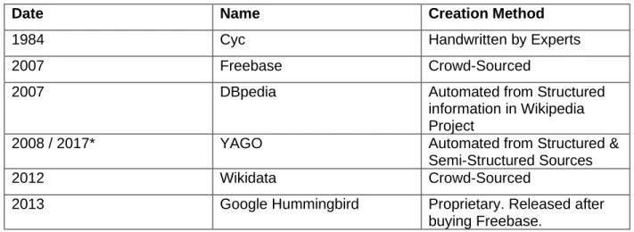
2.1 Date and creation method of knowledge graphs ... 17

2.2 A comparison of knowledge graph components ... 18

4.1 Embeddings and their loss functions ... 38

5.1 Knowledge graph embeddings ... 39

5.2 Mean hit at 10 for TransE and TransM on freebase15k ... 45

5.3 Comparison of TransE, RESCAL, and HolE ... 46

List of Figures

Figure Page

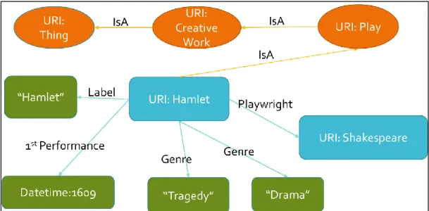
2.1 KG showing information on the entity URI: Hamlet ... 14

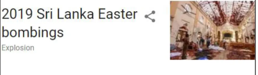
2.2 Google’s knowledge graph card ... 15

2.3 DBpedia entry for Michael Schumacher ... 20

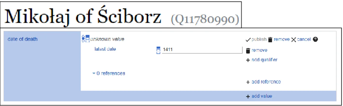
2.4 <Mikołaj of Ściborz, date of death, unknown value> ... 21

3.1 Information extraction flowchart ... 25

3.2a LSTM Forget gate ... 29

3.2b LSTM Input gate ... 29

3.2c LSTM Output gate ... 29

4.1 Embedding input ... 35

5.1 3CosAdd for a-a'+b≠b' ... 42

5.2 TransE embedding with translation vector r ... 43

List of Equations

Equation Page

4.1 Pointwise square error loss ... 38

4.2 Pairwise hinge loss ... 38

4.3 Pointwise hinge loss ... 38

4.4 Pointwise logistic loss ... 38

5.1 Scoring function of RASCAL ... 41

5.2 ComplEx scoring function ... 47

Chapter 1: Introduction

Knowledge graphs contain knowledge of the world in a format that is usable to

computers. A knowledge graph is a directed graph. The nodes of the graph represent named objects such as Abraham Lincoln, concepts such as Gravity, or literal values such as Datetime: March 29, 2019. The edges represent relationships between nodes such as PresidentOf. Knowledge graphs have a wide variety of uses in artificial intelligence fields such as search, question answering, opinion mining, and topic indexing.

Although the idea behind the knowledge graph was first proposed in the 1980s, it was the announcement of Google’s knowledge graph in 2012 that popularized the field [1, p. 1]. Google Hummingbird was released the following year with the motto of

searching for “things not strings”. The use of a knowledge graph is the reason a Google search for hotel gives comparable results to a search for lodging. Knowledge graphs may contain general information about the world or be restricted to a certain subject such as medicine.

Knowledge graphs can be transformed into a dense representation known as a

knowledge graph embedding. Knowledge graph embeddings encode the semantic

meaning of objects and relationships in a low-dimensional space. An object is

represented by a vector. The two vectors representing latte and cappuccino are similar as the objects are similar.

Knowledge graph embeddings make knowledge graphs more usable. Usually, knowledge graphs are stored by mapping the graph’s nodes and edges to an index [2, p. 1]. This method works well for storage but has problems with both inextensibility

and computational inefficiency [2, p. 1]. Multiple knowledge graphs can also be embedded in the same space. This facilitates embedding multimedia information.

Knowledge graphs cannot possibly be complete, that is contain information about every object/concept in the universe. Even a knowledge graph restricted to Shakespeare’s plays could never contain every commentary written or image created. Knowledge graphs were initially created by both crowdsourcing and extracting information from Wikipedia and other sources containing structured or semi-structured information. An example of a structured source is Wikipedia’s infobox, which acts as a table of directed edge, node pairs. A Wikipedia page itself is semi-structured as the title of the page is the name of the node it describes. Using sources such as Wikipedia results in

knowledge graphs that primarily contain frequently mentioned properties of frequently mentioned entities [3, p. 1]. Wikipedia growth has plateaued, so further knowledge needs to be extracted from other sources [3, p. 1].

The incompleteness of knowledge graphs means that they are used as a semantic backbone in combination with other resources [4, p. 36].Knowledge graph coverage can be increased using machine learning and unstructured text. The problem with this approach is that facts extracted from unstructured texts are often wrong [3, p. 1]. Using knowledge graph embeddings, the likelihood of newly extracted data can be calculated based on already-categorized knowledge [3, p. 1]. Only facts calculated to be more probably than some cutoff value will be added to the knowledge graph.

Knowledge graphs embeddings can also increase knowledge graph coverage with reasoning. The added efficiently of knowledge graph embeddings aids the discovery of patterns and rules. Calculating the similarity of two nodes by comparing

their nearest neighbors and directed edges is less efficient and less accurate than comparing their vector representation. The newly discovered patterns and rules are used to automatically fill in information missing from the knowledge graph.

The intended readers of this paper include those who have little or no exposure to knowledge graphs. There is basic, common knowledge to those in the field that is necessary to understand the various researched techniques. For this reason, we first describe the basic components of the knowledge graph. A typical structure is discussed along with different modifications sometimes made to that structure. Then we give a brief overview of how knowledge is extracted from text and then turned into structured data that can be added to the knowledge graph. By discussing the typical extraction process, later discussions of separate components will be placed in their proper context. The discussion of knowledge graph embeddings starts with background knowledge about embeddings. For example, most knowledge graph embeddings first simplify the knowledge graph to a three-dimensional matrix before performing any calculations. Next several types of embeddings are discussed in chronological order. It is not possible to discuss every embedding algorithm given the sheer number, so the more popular types were chosen [2] [5] [6]. The concluding section covers the advantages of using a

knowledge graph embedding instead of the original knowledge graph. Different steps of knowledge base population are improved using knowledge graph embedding.

Applications such as question answering also benefit. Knowledge graphs may store

more information than their embeddings, but knowledge graph embeddings are what make the information more easily usable.

Many of the papers we reference refer to a knowledge base instead of

knowledge graph. Knowledge graph completion and knowledge base completion refer to the same area of research. Conversely, knowledge base population is a

well-explored area of study, but knowledge graph population is not. The term knowledge graph will be used unless, as in knowledge base population, this usage would inaccurately label the field of study.

Chapter 2: Knowledge Graph Components

A knowledge graph contains knowledge about the world in a format that is usable to a computer. Knowledge is defined in terms of objects, concepts, literal values, and the relationships between them. The representation of these in graphical form is covered in this section.

2.1 Entity

A common definition of an entity is an object or concept that can be distinctly identified. Each entity is designated a unique URI or uniform resource identifier and can be assigned string labels. This identification distinguishes Paris Hilton, paris the city, and Paris the Trojan as distinct entities. It also allows for multiple labels such as Elvis, Elvis Presley, and King of Rock that all refer to the same entity. The URI gives entity-based models an advantage over models reliant on string matching such as those created by the popular software Word2Vec.

There are two main types of entities: concepts and named entities. Concepts are abstract ideas such as gravity, distance, or peace. Named entities are those entities that can be referred to using a proper name such as Hamlet, Shakespeare, or the United States. Named entities are real world objects such as a person, location, or event. Most research is focused on named entities. The constant addition of named entities is needed to prevent knowledge graph from become more and more outdated. Entities can also be referred to as instances of a class. Classes are a way of

fundamental interaction as well as an instance of class physical phenomenon [7]. Likewise, in

Figure 2.1, Hamlet is an instance of the class Play and Play is a subclass of

Creative Work. Classes are usually determined by a manually-created schema with more popular schemas allowing easier integration with other knowledge bases. Popular shared schemas are available online at http://www.Schema.org and

https://github.com/iesl/TypeNet.

A knowledge graph focuses on named entities, their properties, and their

relationships [4, p. 38]. In contrast, an ontology focuses on classes, their properties, and

their relationships. For example, an ontology may not contain named wine brands such as Sherry. It would instead define shared properties of the class Wine such as

MadeFromGrapes and IsA Fruit. Knowledge graphs contain some ontological data as seen in the example of <Hamlet, IsA, play>.

There is another type of entity called an event. An event models an occurrence that happened at a specific moment in time.

Figure 2.2 shows that the Google knowledge graph classified the 2019 Sri Lanka Easter bombings as an entity. Google displays entity information as a box on the right-hand side of the search result page in what is known as a knowledge graph card. Events are often extracted from news stations or social media sources such as Twitter. News summation relies on events. Currently even state-of-the-art event extraction is limited to recognizing and categorizing using domain-specific methods [8, p. 1]. Research is also focused on linking events together. Modeling events is a popular enough area of research to have its own standalone component in the 2017 Text Analysis Conference [9, p. 1].

2.2 RDF

A Resource Description Framework (RDF) is commonly used in knowledge

graphs. Each RDF is a triple consisting of <subject, predicate, object> where the subject is an entity’s URI and the object is either a URI, or a literal. An example of a triplet from

Figure 2.1 is <URI: Hamlet, 1st _{Performance, Datetime: 1609>. In}

other words, RDF is two nodes connected by a labeled, directed edge. The RDF structure is effective in representing data but is hard to manipulate due to the symbolic nature of the triplets [10, p. 1].

The expressiveness of the RDF triplet is dependent on the vocabulary of predicates used in the knowledge graph [4, p. 39] Gardner and Krishnamurthy have difficulties with limited predicate vocabulary while using the knowledge graph Freebase to answer questions about Democratic front-runners. Question answering systems use the knowledge graph’s manually produced schema to map questions into queries. As

front-runner is not a participle contained in the schema, the parsers do not work in this scenario [11, p. 1].

RDF is only used for entities or instances. RDFS, or RDF schema, is used for classes. Classes can have properties, which is like predicates. RDFS is lightweight with a more limited vocabulary. OWL [12] and SKOS [13] are alternative, more extensive schemas that build on RDFS and allow for more structured logic for ontological modeling [4, p. 40].

The RDF triplet contains a source entity, a predicate, and an object entity or literal value. Many knowledge graphs expand this triplet to contain additional

information. Before explaining these additions, five common knowledge graphs are discussed to provide background knowledge.

2.3 Different Knowledge Graphs

Five of the most well-known, publicly available, unspecialized knowledge graphs are DBpedia, Freebase, OpenCyc, Wikidata, and YAGO. Some of the differences are due to the date and method of creation as shown in Table 2.1.

Table 2.1: Date and creation method of knowledge graphs.

Date Name Creation Method

1984 Cyc Handwritten by Experts

2007 Freebase Crowd-Sourced

2007 DBpedia Automated from Structured information in Wikipedia Project

2008 / 2017* YAGO Automated from Structured & Semi-Structured Sources

2012 Wikidata Crowd-Sourced

2013 Google Hummingbird Proprietary. Released after buying Freebase.

* First Stable Release

Färber, Ell, Menne, Rettinger, and Bartscherer have performed an in-depth comparison of DBpedia [14], Freebase [15] [16], OpenCyc [17], Wikidata [18], and YAGO [19]. Each knowledge graph was created with different rules in place regarding vocabulary. These rules result in significant differences between the knowledge graphs in the vocabulary of relations, predicates, and classes as seen in .

Table 2.2. In this table relations are used on the class level, while predicates are used on the instance level [20, p. 20].

Table 2.2: A comparison of knowledge graph components [20, p. 25].

DBpedia Freebase OpenCyc Wikidata YAGO

# of Triplets 411,885,960 3,124,791,156 2,412,520 748,530,833 1,001,461,792 # of Classes 736 53,092 116,822 302,280 569,751 # of Relations 58,776 70,902 18,028 1874 106 Unique Predicates 60,231 784,977 165 4839 88,736 # of Named-Entities 4,298,433 49,947,799 41,029 18,697,897 5,130,031 # of Instances 20,764,283 115,880,761 242,383 142,213,806 12,291,250 Avg. # of

Named-Entities per Class

5840.3 940.8 0.35 61.9 9 Unique Non-Literals in Object Position 83,284,634 189,466,866 423,432 101,745,685 17,438,196 Unique Literals in Object Position 161,398,382 1,782,723,759 1,081,818 308,144,682 682,313,508

OpenCyc is the open-source version of Cyc. Cyc was created in 1984 with the goal of encoding common sense knowledge such as people smile when they are happy. Because of this, OpenCyc contains mainly ontological data, not named entities. It is the only knowledge graph with a larger number of relations than number of predicates. It also has the lowest average named-entities per class at 0.35. OpenCyc is curated, or

created by experts. These experts manually encode the information and insert it in the knowledge graph. As this paper focuses on the machine learning side of knowledge graph research, OpenCyc will not be further discussed.

The insertion of relations and predicates is done slightly different on all four remaining knowledge graphs. Freebase was curated by community members with the ability to arbitrarily insert new relations. .

Table 2.2 shows that Freebase has the most relations and predicates, but many of those are not useful. A third of its relations are declared to be inverses of other relations using the markup owl:InverseOf [20, p. 21]. An example of an inverse relation is <Wine, MadeFrom, Grapes> and <Grapes, MadeInto, Wine>. Inverse predicates can also occur. An additional 70% of Freebase’s relations are not used at all. 95% of Freebase predicates are only used once. The inverse relations and predicates of Freebase can lead to misleading results when used to test relation and predicate prediction algorithms. If a relation is removed but its inverse is not, the missing relations can be found by inverting the triplets. Additionally, Freebase is becoming outdated. The knowledge graph was made read-only as of March 31, 2015.

Wikidata is also curated by a community but new predicates are only accepted by the committee if, among other criteria, it is predicted to be used over a hundred times. This limitation puts Wikidata at only 4839 unique predicates. The number of relations is also a low 1874. DBpedia, in contrast, has 58,776 relations created from Wikipedia using an Infobox:Extractor [20, p. 21].

YAGO is constructed by machine learning instead of crowd sourced. It has the fewest relations at 106. By using wildcard characters, it avoids the need for both

birthDate and dbobirthYear. Given YAGO’s ability to extend the triplet to store temporal and spatial information, it avoids dedicated relations such as

distanceToLondon or populationAsOf [20, p. 22]. Interestingly, YAGO has the second largest number of predicates at 88,736.

There is also a difference in the creation of classes. YAGO automatically creates classes from structured and semi-structured sources. As a result, YAGO has 569,751

classes with an average of 9 named-entities per class. DBpedia, which manually

creates classes, has only 736 [20, p. 23]. There are many non-structural differences that also affect knowledge graph choice. An example is the number of knowledge graph entities related to a specific subject such as music. How often the knowledge graph is updated is also a consideration. Further discussion of knowledge graph choice is outside the scope of this paper.

2.4 Adding Additional Information to the RDF Structure

Different knowledge graphs have different modification to the RDF triplet. The vocabulary of predicates typically does not allow for distinctions between past and current relationship. For example,

Figure 2.3 shows how in DBpedia Michael Schumacher is assigned to the category of entities Ferrari_Formula_One_ drivers. There is currently no way in DBpedia of specifying that Michael Schumacher was driving for Ferrari but is not anymore [4, p. 39]. DBpedia can store a limited amount of temporal information using classes like career station which is a subclass of TimePeriod. Still, DBpedia lacks the ability to store the validity period of a statement [20, p. 32].

Not all knowledge graphs share this difficultly with temporal information. Wikidata and YAGO both have the ability to store temporal information by describing the triplet with additional relations such as latest date [20, p. 32].

Figure 2.4 shows the qualifier <latest date, 1411> that acts as metadata for the typical RDF triplet <Q11780990, date of death, unknown value>. In this case, unknown value is a blank node. Freebase is also capable of storing temporal information using compound value types [20, p. 32].

Figure 2.4: <Mikołaj of Ściborz, date of death, unknown value> [21]. Blank nodes like the one in

Figure 2.4 are another way that RDF can store more complicated information. Blank nodes are present in Wikidata and OpenCyc, but not in Freebase, DBpedia, YAGO [20, p. 25]. A blank node indicates a value exists without identifying what it is. It distinguishes between information that is missing from the knowledge graph and

information that is not known. Each blank node must be unique and is assigned its own identifier.

Metadata relating to the triplet is also retained. YAGO allows temporal and spatial information about relations. Also, each triplet in YAGO has a confidence value,

or the calculated probability that the triplet is correct [22]. This confidence value is present because YAGO is generated using machine learning, as opposed to hand generation by crowdsourcing or experts. As additional information is extracted from text or other sources, the confidence value may be adjusted.

Another optional field is a reference. This can be seen in

Figure 2.4’s references field. Wikidata does not have a limit on the number of

references. For example, there are four sources cited for the triple <Brad Pitt, sex or gender, Male> [23]. Another type of reference is provenance, or a justifying sentence. This is not always possible depending on the method of knowledge graph completion. For example, given the triplets <Sarah, MotherOf, Claire> and

<Claire, MotherOf, Sam> the triplet <Sarah, GrandmotherOf, Sam> maybe be generated without textual evidence. Knowledge graph designers specify what information is stored in the knowledge graph.

2.5 Section Summary

To summarize, the descriptiveness of knowledge graphs is determined in part by the vocabulary used. This includes the vocabulary of relations, the vocabulary of

predicates, and the vocabulary of classes. No knowledge graph has restrictions on the number of entities. The size of each of these vocabularies depends on if the knowledge graph is crowdsourced, constructed using machine learning, crowdsourced with

the inverse relations of Freebase does not increase the knowledge that can be represented by the knowledge graph.

Traditionally, information is stored in the knowledge graph as a triplet. Some knowledge graphs such as YAGO extend the triplet to store additional information such as special and temporal data. The goal of knowledge base population is to increase the number of named entities and the number of relations between different entities without adding incorrect information.

Chapter 3: Knowledge Base Population

Knowledge base population consists of building or extending a preexisting knowledge base from text. Knowledge base population needs to be able to add both new entities and new relations. Knowledge graphs constructed by machine learning usually use structured or semi-structured data sources such as Wikipedia. As

Wikipedia’s growth has plateaued there is a need for an alternate method of knowledge graph completion [3, p. 1]. This section discussed extracting knowledge from

unstructured text.

3.1 Supervised Learning

Information extraction is commonly done using supervised learning. Supervised

learning involves neural networks trained on substantial amounts of hand-annotated

data. In many real-world scenarios such high-quality data is scarce [24, p. 2]. Paying experts to hand-annotate data is expensive and therefore not always an option. If enough data is available, it might not be statistically diverse. Additionally, tasks such as entity linking need to handle entities that do not occur in the training data. A neural network trained on medical documents might link an audio recording about Paul Bunyan to the entity bunion, a part of the foot. A common focus of research involves replacing supervised neural networks with semi-supervised, and unsupervised learning. Unsupervised refers to unlabeled training data and semi-supervised networks refers to partially labeled. Ideally, the results will be comparable to what is obtained by the supervised model. Still, even a less effective semi-supervised method will be useful in situations where not enough labeled data is available.

3.2 Syntactical Preprocessing Steps

The effectiveness of information extraction tasks is dependent on the pre-processing of the textual input [25, p. 1]. These steps deal with the syntax of the sentence.

Figure 3.1 shows a flowchart from going from unstructured text to new relations.

Figure 3.1: Information extraction flowchart [25, p. 2].

According to Singh, the first step involves breaking the text up into individual sentences [25, p. 2]. While this may speed up and simplify processing, it has the

disadvantage of preventing the extraction of inter-sentence relations. Then tokenization happens. Tokenizing breaks up words into individual parts that have semantic value. Some words like relight would be broken up into smaller sections re and light. The words are then tagged with the part of speech such as noun phrase.

Stemming or lemming occurs after the part of speech tagging. Stemming

attempts to find a base form of the word by chopping off parts such as running to run. Lemming uses a vocabulary and morphological rules. Negation processing also

happens. This would involve replacing phrases such as not less than with

greater than.

Lastly entity reorganization occurs. This refers to classifying all entities into predefined categories. For example, an entity could be categorized as a person, organization, location, or miscellaneous. This step is sometimes combined with entity disambiguation.

3.3 Entity Disambiguation

Entity disambiguation is the task of connecting any mention of an entity in text to

its corresponding entity. Entity disambiguation is also termed named entity linking and

named entity disambiguation. This task is the subject of much research. More recent

methods use knowledge graph embeddings.

There are several difficulties with entity disambiguation. Multiple entities might share the same label. For example, paris could refer to Paris Hilton; Paris, France; or Paris of Troy. Additionally, one entity may also have multiple labels such as Elvis Presley and King of Rock ‘n’ Roll. Entity disambiguation also needs to handle new entities that are not yet in the knowledge graph. In some cases, the supposedly new entity may be a new label for a preexisting entity. It is difficult for artificial intelligence to distinguish between an unseen entity or an unseen label. In some cases, a label is not used to describe an entity. The text may contain

phrases such as “the book previously mentioned”. Coreference resolution attempts to determine if multiple words in a text refer to the same entity. Coreference resolution is considered one of the most difficult tasks in language understanding [26, p. 1]. This is because understanding the sentence may require outside knowledge. Vincent Ng uses the example of “The Queen Mother asked Queen Elizabeth II to transform her

sister, princess Margaret, into a viable princess by summoning a renowned speech therapist, Nancy Logue, to treat her speech impediment” [26, p. 1]. The first her

requires knowing that Princess Margaret is Queen Elizabeth II’s sister. The second her

requires the commonsense knowledge. Nancy Logue would not be summoned to treat herself. This is a necessary preprocessing step before relation extraction.

3.4 Relation Extraction

In relation extraction or link prediction, links are predicted with a certain

probability. Links with a higher probability than some number p1 will be added to the graph. YAGO stores this probability as part of the relation. Newly extracted information may cause previously predicted relations to be adjusted. Relations less probable than

p2 may be removed from the graph or flagged for manual review.

The text does not need to explicitly mention a predicate for the relation to be extracted. For example, the text Samuel Smith went to school in New York

should provide a probably well above zero for <Samuel Smith, born-in, New York> [27, p. 257]. This probability may be increased by multiple occurrences in the text. Eventually the probability may exceed some threshold and the triplet be added to the knowledge graph without any direct textual evidence.

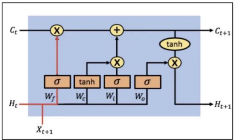
3.5 Long Short-Term Memory (LSTM)

LSTM and variations on LSTM are by far the most popular form of neural network used in information extraction. Traditional recurrent neural networks suffer from the vanishing or exploding gradient problem. The long-term components may either grow exponential fast compared to short-term components or change exponentially fast to norm 0 [28, p. 2]. What happens is dependent on the relative size of largest eigenvalue of the recurrent weight matrix [28, p. 2].

LSTM solves this problem. Long Short-Term Memory has three gates: the forget

gate, the input gate, and the output gate. These can be seen in

Figure 3.2a: LSTM Forget gate which highlights in turn the forget, input, and output gates. The C on the top represents the current cell state, H represents the neural network’s hidden layer, and x is the input for that specific layer. This input could be a word in a sentence like the word hot from Brandon felt hot. Other options involve inputting n characters at a time such as n fel or n words at a time such as

felt hot. This input may have also been preprocessed using techniques such as stemming or lemming.

Figure 3.2a: LSTM Forget gate.

Figure 3.2b: LSTM Input gate.

The forget in 3.2a takes in the hidden state from the previous cell and that timestep’s input. The two inputs are multiplied by a weight matrix, a bias is added, and then a sigmoid function is applied. This results in the previous cell state being multiplied by a vector with values between 0 and 1. Some numbers in the cell state will be

multiplied by 0 and completely forgot, some will be multiplied by 1 and completely remembered, and some will be partially remembered.

Similarly, the input gate in Figure 3.2b uses a sigmoid function as a filter. The tanh function creates a vector of all possible values that can be added given that timestep’s input and the previous hidden state. The sigmoid function multiplied the potentially added information by a vector with values in the range (0, 1).

The output gate in Figure 3.2c works almost identically to the input gate. The tanh function is applied to the cell state after it is updated by the input gate. The output gate controls how much of the cell state, previous hidden layer, and current input is outputted to the next hidden layer.

Bidirectional Long Short-Term Memory (BiLSTM) is one of the more popular

variations of LSTM. In this method two LSTMs are used. One is given the data from beginning to end and the other is given data from the end to beginning. The output of the LSTMs is combined after each step. In many cases BiLSTM learns faster than the LSTM approach. BiLSTM has eight sets of weight in comparison to the four sets of LSTM.

3.6 Categorical Data and Keras

Categorical data cannot be directly added to a neural network. A common method of dealing with categorical data is one-hot encoding. That is, for each category a dummy variable is created with the value of either zero or one. For categories with a large enough vocabulary such as words, the resulting matrix is too large to be practical. A popular alternative is to create an embedding layer with the API, Keras.

Keras is one of the most popular deep learning frameworks. As an API, Keras makes is simpler to use other machine-learning software libraries such as TensorFlow. Using Keras, adding an additional embedding layer just takes one line of code.

Activation functions, loss functions, and metrics are changed by replacing a single string.

Creating an embedding layer requires the number of input dimensions di, the

number of output dimensions do, and the sequence length. The sequence length is how

many words, for example, to encode at one time. The resulting layer can be thought of as a lookup table with a random initialization similar to random weights. Each possible input is represented by a vector of length do. If di = do, the resulting embedding will be

identical to the one-hot matrix. It is important to mark this layer as non-trainable so that the same words consistently are represented by the same vector. An embedding layer is a scalable method of dealing with categorial data.

3.7 Preventing Overfit

LSTM networks tend to overfit. One traditional way to decrease overfitting is to train multiple neural networks and average the different models’ predictions. This solution works poorly for many LSTMs given the time it takes to train large networks. In

2014 dropout was proposed as a solution to overfitting. During training, units and their connections will be randomly dropped. This was found to significantly reduce overfitting and the resulting neural network produced better results than other methods of

regularization such as the before mentioned averaging [29, p. 1]. Dropout is the most common method of preventing overfitting mentioned in the papers reviewed. It can be implemented in one line of code using Keras. The model is told what percent of nodes to drop. Despite the benefits of using dropout, a stop condition still needs to be used. The condition could be a limit on epochs or when the model fails to improve on the validation set.

3.8 Noise in Extracting Data from Unstructured Text

Extracting information from the web often produces noisy and unreliable relations [3, p. 1]. Google researchers designed the Knowledge Vault to judge the probability of new facts. It calculates the probability of the new fact based on the data extracted from the web. It also calculates the probability of the new fact based on the facts already present in Freebase. Fusing these two probabilities results in a more accurate

probability estimate [3, p. 2]. Low probability facts should be removed if already present in the knowledge graph and high probability facts can be added. Given the high

precision required by Google, removal and addition may only happen after manual review.

3.9 Judging Accuracy of Techniques

Knowledge base completion has the goal of adding missing true triplets while avoiding adding false triplets. Glass and Gliozzo [27] discuss three popular methods for evaluating knowledge base population. In held-out some tuples are removed from a

pre-existing knowledge base. These removed tuples must be predicted. Any predicted tuples not in the knowledge graph are considered incorrect. The system could, of

course, correctly predict a tuple not in the knowledge graph. There is also no guarantee that the removed tuples are in the corpus. However, if multiple systems are used to evaluate the corpus these absent tuples will not be found by any systems. If the system is judged by its relative effectiveness compared to a benchmark, tuples not in the

corpus will have no effect.

The second method discussed by Glass and Gliozzo involved exhaustively annotating all tuples in the corpus [27]. This involves a large amount of manual effort. It also does not work for evaluating triplets not directly present in the text. Earlier it was discussed how Samual Smith going to school in New York increased the probability that Samual Smith was born in New York. The third method involves pooling the tuples produced by multiple systems then manually determining if each tuple is correct [27, pp. 259–260]. The amount of manual effort per system depends on the number of systems pooled. All three of these methods are used to judge the performance of trained neural networks. The effectiveness of neural networks used with embedded knowledge graphs can likewise be evaluated.

Chapter 4: Embedding Background Knowledge

Knowledge graph embeddings are useful because the embedding encodes semantic information about the entities and relations. This is far more extensible and computationally efficient than traditional methods of storing entities and relations by index mapping [2, p. 1]. The previous knowledge graph is changed into a dense representation in a multi-dimensional space. Each embedding and relation is

represented by a vector. The optimal number of dimensions of the knowledge graph is determined by increasing the dimensions of the model until the model is no longer improving. The resultant embedding can be used to easily compute the similarities between entities or relations.

There are countless types of knowledge graph embeddings. Knowledge graphs may contain millions of nodes and billions of edges. Because of this, it is important that the embedding scoring function be at worst O(n) where n is linear in respect to the size

of the knowledge graph [6, p. 1]. The number of model parameters is also a factor when choosing an embedding method. Many types of embeddings are designed to better model some facet of the knowledge graph. The simpler TransE cannot model complex relations [2, p. 11]. TransG seeks to model relations that have multiple meanings when involving different entity pairs [2, p. 18]. Modeling additional features makes the model more accurate, but more complicated embeddings are more computationally expensive to use as well as create.

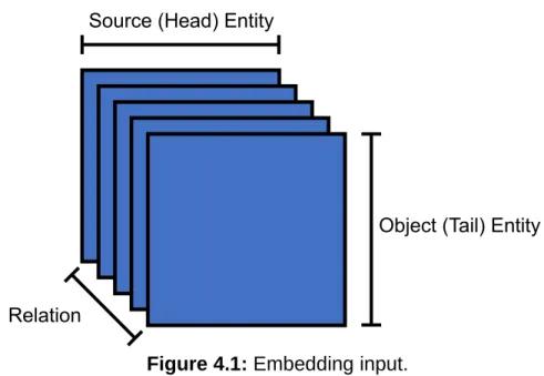
4.1 Initial Input

Before embedding a knowledge graph, the information contained in the

the neural network to process. A common input is a three-dimensional matrix as seen in Figure 4.1. Directed edges between two entities are added to the matrix. The arrow of the edge points from the source/head entity to the object/tail entity. The matrix contains values {0,1}. A one means that there is a relation between the source and object entity and a zero means that there is no relation. The object entity is where the directed edge points. If the matrix is taken as Eh x Et x R, then Eh(i) = Et(i). In other words, the same

position is assigned to the same entity in both dimensions. This improves the resultant embedding. A large amount of knowledge is lost by this transformation such as literal values and metadata about the RDF pair. Still, even with this loss of information

embedded knowledge graphs show superior performance on a variety of tasks. Specific examples will be shown later when discussing the use of embeddings.

Figure 4.1: Embedding input.

4.2 Relationship Categories

Relationships are generally divided into four categories: 1:1, 1:n, n:1, and n:n

where the first refers to the head entity and the second to the tail entity. An example of Source (Head) Entity

Object (Tail) Entity

1:n is <United States, HasPresident, x> where xcould refer to multiple entities. n:1 is the reverse <x, HeldOffice, president>. Only roughly 26% of triplets are 1:1 relations [30, p. 329]. For this reason, a knowledge graph embedding such as TransE that cannot accurately model complex relationships is less accurate.

4.3 Negative Sampling

Training a knowledge graph embedding requires negative examples. These are often created by randomly replacing either an entity or a relation with another randomly selected. Yankai, Han, Xie, Liu, and Sun discussed two issues with this method. If the nationality entity from the tuple <Steve Jobs, nationality, United States>

was replaced with a random entity to form the triplet <Steve Jobs, nationality, Bambi>, this would not fully train the model. If Steve Jobs was replaced with an entity of the same type, that is a person, this could also cause issues. <Bill Gates,

nationality, United States> may be generated as a negative training example when this fact is true. For a 1:n relationship like nationality : person the 1 side should be replaced to reduce the likelihood of a false negative [2, p. 29].

4.4 Loss Functions

Knowledge graphs are embedded using a neural network. The error of an individual relation is calculated using a scoring function specific to the embedding. The scoring functions are then combined using a loss function. There is a large amount of research in developing new scoring functions, but very little on loss functions [31, p. 2]. The scoring functions of HolE and ComplEx have been proven equivalent, but their

performance is still different [31, p. 2]. A likely explanation for this difference is the different loss functions of the two embedding types.

The following definitions are used in the loss functions. l(x) = 1 if x is true and -1

otherwise where x is the RDF triplet. Similarly, for pairwise functions, f(x)refers to a true triplet and f(x’) a false triplet. The margin parameter λ is a hyperparameter. Finally, [x]+

is defined as the max (x, 0).

A hyperparameter such as λ is not tuned by the neural network. Like the number of embedded dimensions, λ is tuned based on the performance of the resultant

embedding. This adds another level of optimization to those embedding models that use λ.

Four different loss functions are used by the discussed embeddings as defined in Equation 4.1, Equation 4.2, Equation 4.3, and Equation 4.4. RESCAL uses Pointwise Square Error Loss. The goal is to minimize the squared difference between the score and the expected output [31, pp. 2–3]. This equation benefits from not having the margin hyperparameter. TransE and TransM instead use the Pairwise Hinge Loss. The goal is to maximize the difference of the positive and negative examples by a good margin [31, p. 4]. HolE with the Pointwise Hinge Loss instead aims to minimize negative scores to - λ and maximize positive scores to + λ [31, p. 3]. Lastly, ComplEX uses

Pointwise Logistic Loss. This results in a smoother loss slope than the Pointwise Hinge Loss with the advantage of avoiding the λ hyperparameter.

Table 4.1: Embeddings and their loss functions [30, p. 331] [31, pp. 2–4].

Embedding Type Loss Function

RESCAL Pointwise Square Error Loss

TransE Pairwise Hinge Loss

TransM Pairwise Hinge Loss

HolE Pointwise Hinge Loss

ComplEx Pointwise Logistic Loss

Equation 4.1: Pointwise square error loss [31, p. 2].

L =

1

2

∑ (f(𝑥) − l(𝑥))

2 𝑥 ϵ 𝑋

Equation 4.2: Pairwise hinge loss [31, p. 4].

L = ∑

∑ [ λ + f(𝑥′) − f(x)]

𝑥′∈ 𝑋− 𝑥 ∈ 𝑋 +

Equation 4.3: Pointwise hinge loss [31, p. 3].

L = ∑ [ λ − l(𝑥) ∙ f(𝑥)]

𝑥 ∈ 𝑋

Equation 4.4: Pointwise logistic loss [31, p. 3].

L = ∑ log(1 + exp(−l(𝑥) ∙ f(𝑥)))

There are additional, undiscussed loss functions commonly used in knowledge graph embeddings. When designing a new type of embedding, the designers need to decide on a loss function as well as a scoring function for their model.

Chapter 5: Embedding Types

There are numerous types of embeddings. Knowledge graphs such as YAGO, DBpedia, and Freebase contain millions of nodes and billions of edges [6, p. 1]. For this reason, knowledge graph embedding techniques must be scalable. Time complexity, space complexity, and the accuracy of the representation are all crucial factors in choosing an embedding.

The five types of embeddings discussed are listed in Table 5.1. In this table, n is the number of entities, m is the number of relations, and d is dimensionality of the

embedding space. RESCAL was an important early embedding but is no longer used due to the prohibitive time complexity of O(d2_{). TransE is popular due to its simplicity}

and efficiency but is crippled by its inability to model complex relations. TransM is one of many TransE extensions that attempt to improve the embedding quality. HolE and ComplEx both embed the knowledge graph using complex numbers. An alternate way of training HolE was proposed in 2017 and reduced the time complexity to O(d).

Table 5.1: Knowledge graph embeddings [5, p. 2732].

Date Name Space Complexity Time Complexity

2011 RESCAL O(nd + md2_{) O(d}2₎

2013 TransE O(nd + md) O(d)

2014 TransM O(nd + md) O(d)

2015 HolE O(nd + md) O(d log d)

2016 ComplEx O(nd + md) O(d)

A common method of comparing knowledge graph embeddings is calculating the mean hit at ten. If the desired object entity one of the ten closest entities, then it counts as a hit. The relative accuracy of different knowledge graph embeddings is compared. Different researchers categorize knowledge graph embeddings differently. One way is to divide the embeddings into translational distance models and semantic matching models [5, p. 2725] [26, p. 2725]. TransE is a translational distance model as its scoring

function is distance-based [26, p. 2725]. The likelihood of a triplet being correct is calculated by translating the source entity vector by the relation vector. The closeness of the resulting vector to the object entity vector determines the probability.

RESCAL, HolE, and ComplEx are all semantic matching models. The scoring functions of semantic matching models are similarity-based [5, p. 2725]. These

functions compare the latent semantics of entities and relations. A latent feature is not directly observed in the data. For example, Alec Guinness received the Academy Award because he is a good actor. Being a good actor is a latent feature [6, p. 6]. This latent feature can be calculated from observed features such as how much money the actor’s movies made. The first latent feature model discussed is the oldest of the five,

RESCAL.

5.1 RESCAL

RESCAL defines each entity with a vector that represents the entity’s latent features. As it uses a tensor product, the time complexity is O(d2_{). The scoring function}

of RESCAL is shown in

Equation 5.1. Each relation is represented by a weight matrix W_k ∈ ℝd ×d _where 𝑤𝑎𝑏𝑘 describes how much latent features 𝑎 and 𝑏 interact in relation 𝑘. [6, p. 6] 𝑑 is the

number of dimensions of the embedding. Vectors 𝑒𝑖 and 𝑒𝑗 are two vectors that

represent the latent features of entity 𝑖 and entity 𝑗 respectively. The Loss Function is Pointwise Square Error Loss as calculated by Equation 4.1.

Equation 5.1: Scoring function of RASCAL

fijk= 𝑒𝑖𝑇∙ 𝑊k∙ 𝑒𝑗 = ∑ ∑ 𝑤𝑎𝑏𝑘∙ 𝑒𝑖𝑎 ∙ 𝑒𝑗𝑏 d

b=1 𝑑

a=1

RESCAL is vast an improvement over previous approaches to knowledge graph embeddings. It was the first embedding to have a unique latent representation for each entity [32, p. 3]. Previous entities had a subject representation and an object

representation. The improvement is due to modeling the initial input as a three

dimensional matrix as seen in section 5.1, Figure 4.1 [32, p. 2]. This was revolutionary at the time. RESCAL is no longer used due to a prohibitive time complexity of O(d2_).

The next entity embedding discussed, TransE, was also revolutionary because of its low time complexity of O(d).

5.2 Word2Vec Embeddings

The first translational distance model, TransE, was inspired by Word2Vec. Word2Vec is a popular probabilistic method for embedding strings based on the context. In the training text corpus, if the strings cooccur within a certain number of words, co-occurrence is true. This results in an n by n matrix where n is the size of the

vocabulary. The matrix is turned into a string embedding using a neural network. This technique can be expanded to work to encode n-characters at a time or to encode

This technique is popular both because of the free implementation available online and because of the slightly misleading claim that the word embeddings of king + women – man = queen.

Figure 5.1 shows the inaccuracy of the 3CosAdd technique when the three source vectors are not excluded from the possible answers. The offset of a-a' is small

enough that this equation results in the nearest neighbor of b [33, p. 137]. This

technique is the most accurate for words with near-identical embeddings such as single-plural and male-female.

Figure 5.1: 3CosAdd for a-a'+b≠b' [33, p. 137].

There is another major issue with Word2Vec due to the use of strings instead of entities. The location of words like bat is somewhere between the logical embedding of bat from baseball and bat the animal. The embedding is inaccurate for either usage. Embedding entities instead has numerous applications.

5.3 TransE Embeddings

TransE is one of the most well-known methods of entity embedding. TransE has a time complexity of O(d) which is a drastic improvement over RESCAL’s O(d2_{). Lin,}

Han, Xie, Liu, and Sun discuss TransE in detail. It defines the relation between the head

h and tail t entities using the vector r. This can be seen in Figure 5.2. Each distinct

predicate is represented by a relation r. The scoring function is the simple function

𝑓𝑟(ℎ, 𝑡) = ‖ℎ + 𝑟 − 𝑡‖. When compared to traditional, non-embedded, knowledge

graphs, TransE can model entity and predicate relatedness with fewer model

parameters and lower complexity. TransE shows a significant improvement especially for large scale and sparse knowledge graphs [2, p. 9] [34, p. 2792].

Figure 5.2: TransE embedding with translation vector r [2, p. 9].

TransE uses the pairwise hinge loss function defined by Equation 4.2. The goal of the margin loss function is, again, to maximize the differences of the positive and negative examples by a good margin. The margin is a hyperparameter so also needs to be optimized.

TransE cannot represent complex relationships.If PresidentOf is a distinct vector, George W. Bush ≈ Barack Obama. The embedded knowledge graph does not distinguish between the two embeddings as their location is the same. TransE does not even work for all 1:1 relations. Reciprocal relationships cause the same issue of undistinguishable entities.<Sarah, FriendsWith, Sam> + <Sam,

TransE is popular because of its simplicity and efficiency. It does not create the most accurate knowledge graph embedding. TransE embeds the entities on the n side

of a complex relationship extremely close together [30, p. 330]. This makes it difficult to discriminate between the n entities. For this reason, TransE is often expanded upon to

allow for more complex embeddings. Some examples are TransM, TransH, TransR, CTransR, TransD, TransSparse, TransA, and TransG [2, pp. 11–12].

5.4 TransM Embeddings

The goal of TransM was to improve the performance of TransE without adding significant complexity. Due to the TransE scoring function, entities on the n side of a

complex relationship are trained close together. This makes them harder to distinguish. TransM aims to spread these entities farther apart as seen in

Figure 5.3. In TransM, more complex relations are given a lower weight. The new scoring function is f_𝑟(ℎ, 𝑡) = 𝑤𝑟‖ℎ + 𝑟 − 𝑡‖ [30, p. 330]. TransM uses the same loss

function as TransE, the pairwise hinge loss function. TransM uses the L1-norm as it significantly increase precision compared to the L2-norm [30, p. 336].

Figure 5.3: Modeling 1:n relations in TransE vs. TransM [30, p. 332].

The relation weight, representing the complexity of a relation, is simple to calculate. For a given relation, the number of head entities per distinct tail entity for a given relation can be calculated by summing a Boolean vector in the initial data. The number of tail entities per head entity can be calculated similarly. Let H_𝑡,𝑟 be the average number of head entities per tail entity for a relation and T_ℎ,𝑟 be the average number of tails per head. Then the relation weight is 𝑤_𝑟= log(H_𝑡,𝑟+ T_ℎ,𝑟) −1 [30, p. 331]. As the relation weight is only calculated once, TransM keeps the efficiency of TransE. TransM also achieves its goal of superior performance as shown in Table 5.2.

Table 5.2: Mean hit at 10 for TransE and TransM on freebase15k [30, p. 334].

Task Predicting Subject Predicting Object

Mapping 1:1 1:n n:1 n:n 1:1 1:n n:1 n:n

TransE 59.7% 77.0% 14.7% 41.1% 58.5% 18.3% 80.2% 44.7%

TransM 76.8% 86.3% 23.1% 52.3% 76.3% 29.0% 85.9% 56.7% 5.5 HolE Embeddings

HolE was designed as a knowledge graph embedding that is more efficient than RESCAL and more accurate than TransE. Previously proposed TransE extensions such as TransH and TransR could accurately model complex relations but lost the simplicity and efficiently of TransE. TransR even has the time complexity of O(d2_{) [5, p. 2732].}

Unlike TransE and its extensions, HolE is a semantic matching model.

Instead of using the tensor product which has a time complexity of O(d2_{), HolE}

uses circular correlation with a time complexity of O(d log d). This is possible because

HolE is f_𝑟(ℎ, 𝑡) = 𝑟𝑇_{(ℎ ⋆ 𝑡)) where ⋆ stands for circular correlation. Circular correlation}

can be calculated using the fast Fourier transform ℱ. ℎ ⋆ 𝑡 = ℱ−1( ℱ(ℎ) ⨀ ℱ(𝑡)) where

ℱ(𝑎) stands for the complex conjugate of the fast Fourier transform and ⨀ stands for the elementwise multiplication of two matrices [35, p. 3]. HolE uses the Pointwise Hinge loss function shown in Equation 4.3.

HolE show superior performance to TransE and RESCAL on the WordNet18 and Freebase15k datasets as seen in Table 5.3. All embeddings perform much better on WordNet18 because WordNet18 has only 18 relations. HolE outperforms TransE and RESCAL for five of the six categories. It achieves close to the performance of TransE for the remaining category. HolE is a more accurate representation than TransE or RESCAL with a time complexity less than RESCAL.

Table 5.3: Comparison of TransE, RESCAL, and HolE [35, p. 6].

Data Set WordNet18 Freebase15k

Hits at 1 3 10 1 3 10

TransE 11.3% 88.8% 94.3% 29.7% 57.8% 74.9%

RESCAL 84.2% 90.4% 92.8% 23.5% 40.9% 58.7%

HolE 93.0% 94.5% 94.9% 40.2% 61.3% 73.9%

5.6 ComplEx Embeddings

Like HolE, ComplEx uses complex numbers for the embedding. The motivation behind using complex numbers is different. Embeddings created using dot products are scalable, but cannot handle irreflexive parameters without making the embedding overly complex [36, p. 2]. As dot products are symmetrical, they cannot differentiate between the head and tail of an RDF triplet. The dot product of complex numbers is not

symmetric and so can model irreflexive parameters while remaining scalable. ComplEx takes advantage of this to obtain a time complexity of O(d).

The dot product of a complex number is calculated by the equation 〈𝑢, 𝑣〉 = 𝑢̅𝑇 _⋅ 𝑣. The complex conjugate of 𝐮 is transposed and multiplied by 𝒗. However, the scoring function must return a real number so only the real portion of the dot product is kept. If

𝑐 = 𝑎 + 𝑏i than let Re(𝑐) represent the real portion of 𝑐, that is 𝑎. Let Im(𝑐) represent the imaginary portion of 𝑐, that is 𝑏. The scoring function shown in Equation 5.2 shows how the complex vector dot product can be transformed into the real vector dot product. The loss function of pointwise logistical loss shown in Equation 4.4 is used on the score. Pointwise logistical loss does not contain the margin hyperparameter, which makes ComplEx even simpler to calculate.

Equation 5.2: ComplEx scoring function [36, p. 4].

f _𝑟(ℎ, 𝑡) = Re(〈𝑤_𝑟, 𝑒_ℎ, 𝑒_𝑡〉) = Re (∑ 𝑤_𝑟𝑑 ∙ 𝑒_ℎ𝑑 ⋅ 𝑒̅_𝑡𝑑

𝐷

d=1

)

= 〈Re(𝑤𝑟), Re(𝑒ℎ), Re(𝑒𝑡)〉 + 〈Re(𝑤𝑟), Im(𝑒ℎ), Im(𝑒𝑡)〉 + 〈Im(𝑤𝑟), Re(𝑒ℎ), Im(𝑒𝑡)〉 − 〈Im(𝑤𝑟), Im(𝑒ℎ), Re(𝑒𝑡)〉

ComplEx performs better than HolE or TransE on Freebase15k. However, ComplEx performs almost identically to HolE on WordNet18. As WordNet18 only contains 18 types of relations, the WordNet18 results are less significant. Therefore, ComplEx is more efficient than HolE and produces a better representation than TransE or HolE.

Table 5.4: Comparison of TransE, HolE, and ComplEx [36, p. 7].

Data Set WordNet18 Freebase15k

Hits at 1 3 10 1 3 10

TransE 8.9% 82.3% 93.4% 23.1% 47.2% 64.1%

HolE 93.0% 94.5% 94.9% 40.2% 61.3% 73.9%

Complex 93.6% 94.5% 94.7% 59.9% 75.9% 84.0%

5.7 Spectrally Trained HolE

Hiayashi and Shimbo compared HolE and ComplEx. They proved that the Fourier transform of HolE embeddings is equivalent to a ComplEx embedding with conjugate symmetry. Conversely every ComplEx embedding has a corresponding HolE embedding that is equivalent. Equivalency means that when the two embeddings apply their respective scoring function the same value is produced. Additionally, Hiayashi and Shimbo showed how HolE’s scoring function could be calculated in O(d) time [32, p. 554].

The time limiting factor for HolE is the fast Fourier transform and inverse fast Fourier transform [37, p. 556]. The original scoring function of HolE is f𝑟(ℎ, 𝑡) = 𝑟𝑇∙ (ℎ ⋆ 𝑡). Spectrally trained HolE instead uses the scoring function of f_𝓇(𝒽, 𝓉) = ℱ(𝑟𝑇_∙ (ℎ ⋆ 𝑡)) to find the optimal 𝓇 = ℱ(𝑟), 𝒽 = ℱ(ℎ), and 𝓉 = ℱ(𝑡). In Equation 5.3, ⋆ stands for circular correlation, ℱ stands for the fast Fourier transform, ⨀ stands for the

elementwise multiplication of two matrices, and 𝑥 stands for the complex conjugate of 𝑥. After the training is done, the inverse Fourier transform can be applied to 𝓇, 𝒽, and 𝓉 to find r, h, and t. Using this method, HolE and ComplEx can both be calculated in O(d)

Equation 5.3: The spectrally trained HolE scoring function [37, pp. 555–556]. ℱ(𝑟𝑇∙ (ℎ ⋆ 𝑡)) = 1 d∙ ℱ(𝑟 𝑇_{) ∙ ℱ(ℎ ⋆ 𝑡)} = 1 d∙ ℱ(𝑟 𝑇_{) ∙ ℱ(ℎ ⋆ 𝑡)} =1 d∙ ℱ(𝑟 𝑇_{)(ℱ(ℎ)̅̅̅̅̅̅̅ ⊙ ℱ(𝑡))} = 1 d∙ 𝓇 T_{(𝒽̅ ⨀ 𝓉)}

If ComplEx and HolE are equivalent, why did ComplEx outperform HolE experimentally as seen in

Table 5.4? The two types of embeddings use different loss functions. HolE uses Pointwise Hinge Loss while ComplEx uses Pointwise Logistical Loss. It is also possible that when the experiment was completed a suboptimal margin hyperparameter was used with HolE’s Pointwise Hinge Loss. The experiment predicted the head or tail of a relation. This process is useful for auto-completion of knowledge graphs using

Chapter 6: The Use of Embeddings

Embeddings greatly simplify the use and completion of knowledge graphs. By condensing the information into a dense matrix, the information is easier to use and store. Using a knowledge graph embedding the probability of a relation can be easily calculated using the scoring function. Additionally, a comparison of different entity vectors gives the similarities of different entities. The similarity of relations can be found the same way. The labeled training data needed for tasks such as entity disambiguation can be reduced or eliminated because of these benefits. This section discusses the benefits of using a knowledge graph embedding instead of the knowledge graph itself.

6.1 Abbreviation Disambiguation

Abbreviation disambiguation was previously done by training a neural network on costly hand annotated data. However, this approach does not work for abbreviation not seen in the labeled dataset [38, p. 2]. Embeddings are more flexible. Ciocisi, Sommer, and Assent were able to disambiguate abbreviations using unsupervised learning. Both the embedding and its possible longform were embedded using the surrounding

context. The embedded vectors were compared, and the abbreviation connected to its most similar longform [38, p. 2].

6.2 Relation Extraction

Relation extraction used to be done by semi-supervised learning [39, p. 2246]. That is a neural network trained on both labeled and unlabeled data. It works by a labeled RDF triplet. It then assumes that if the same two entities mentioned in another part of the text, the relation between them is the same [39, p. 2246]. This causes the relation extraction process to be noisy. If Sally was born in Minnesota and Sally

was governor of Minnesota, the relation extractor would believe born and

governor to be equivalent relations.

The solution for improved relation extraction is the same as for abbreviation disambiguation. The sentence embedding is compared to the embedding of all possible relations between the two entities. The most likely is the predicted result [39, p. 2248].

6.3 Link Prediction / Reasoning

Link prediction or reasoning involves inferring that a triplet exists using the information already in the knowledge graph. This can be done easily with knowledge graph embeddings. The scoring function gives the probability that a link is correct [5, p. 2738]. Given a head entity and a relation, the probability of each tail entity can be calculated. This is also useful for evaluating the accuracy of an embedding [5, p. 2738]. Correct triplets should be more probably than incorrect triplets.

6.4 Classifying Entities as Instances of a Class

The relation IsA is part of the knowledge graph embedding. Classification can be treated as a form a link prediction. The head is the entity to be classified and the relation is IsA. The probability that the entity is an instance of different classes can be

calculated and the most likely class found [5, p. 2738].

6.5 Language Translation

Chen, Tian, Yang, and Zaniolo discuss using knowledge graph embeddings for translation. This involves creating separate embedded knowledge graphs for each language. The relations and entities of the different embeddings are aligned. This alignment is done using crowdsourcing in knowledge graphs such as Wikidata and DBPedia [40, p. 2]. The researchers used an extension of TransE and compared three

methods of alignment: distance-based axis calibration, translation vectors, and linear transformations. Linear transformation was the most accurate in their experiment [40, p. 6]. In contrast, a more recent study showed improved performance using an embedding method capable of capturing non-linear alignments [41, p. 147]. Language translation is still an ongoing field of study.

6.6 Recommender Systems

Sparse data is a known problem when working with recommender systems. The solution is to create a knowledge graph embedding containing the items. A book is embedded in a knowledge graph along with its summary and image. The structure, textual, and visual knowledge of the book can be combined to embed the book into a knowledge graph [5, p. 2740]. The user can be recommended books similar to what the user liked in the past. Multiple users also can be embedded into the knowledge graph based on their history. Similar users should like similar books.

6.7 Question Answering

In question answering a question is asked in natural language and answered using the information contained in a knowledge graph. Most questions can be answered by a machine if the question’s corresponding head entity and relation can be identified [42, p. 1]. A word embedding model is used to embed the question’s relation and the question’s entity [5, p. 2739]. These two embeddings are compared with the knowledge graph embedding to find the most likely match. This identifies the question’s

Chapter 7: Conclusion

Knowledge graphs are essential to artificial intelligence. In the words of Google, knowledge graphs aim to represent “things, not strings”. Knowledge graphs provide computers with knowledge of the world in a structured format. This information is necessary to a wide variety of fields in artificial intelligence. Some examples are search, question answering, opinion mining, recommender systems, and language translation. However, knowledge graphs are not well known to those not researching the field. For this reason, we first described knowledge graphs in detail.

We next described knowledge base population. Knowledge base population involves adding additional triplets to knowledge graphs. As the growth of Wikipedia has plateaued, it is more important that this information can be extracted from unstructured text. Traditionally, this has required enormous amounts of hand-annotated data.

Knowledge graph embeddings decrease or eliminate this requirement.

We showed how knowledge graph embeddings have increased in accuracy and decreased in time complexity over the years by discussing popular embeddings.

RESCAL was developed in 2011 with time complexity O(d2_{). In 2013, TransE was}

developed with time complexity O(d). TransE models complex relationships poorly, but

TransE extensions are still popular due to the simplicity and low time complexity of TransE. ComplEx and HolE are both more accurate than TransE with time complexity O(d).

We then discussed the advantages of using knowledge graph embeddings instead of the knowledge graph itself. Knowledge graph embeddings are a dense

matrix. This improves both usage and storage. We showed how the knowledge graph embedding’s scoring function can calculate the probability of a triplet. Another

advantage of embeddings is in calculating the similarities of different entities or different relations. It is easy to compare the similarity of two vectors. We discussed how

knowledge graph embeddings are useful in artificial intelligent fields such as language translation and recommender systems. Our paper shows the importance of knowledge graph embeddings to artificial intelligence research and practice.