THE UNIVERSITY
of
LIVERPOOL
Embedding Approaches for Relational Data
Thesis submitted in accordance with the requirements of the University of Liverpool
for the degree of Doctor of Philosophy
in
Electrical Engineering and Electronics
by
Yu Wu, B.Sc.(Eng.)
Embedding Approaches for Relational Data
by
Yu Wu
Copyright 2018
Acknowledgements
First and foremost, I would like to express my deepest gratitude to my supervisors Dr. Tingting Mu and Dr. Yannis Goulermas, for their patient, encouragement, and professional instructions throughout this research. I could never progress toward the ability to reach to this stage without their consistent and illuminating support.
I would also like to extend my appreciation to my annual progress committee members: Dr. Xu Zhu and Prof. Simon Maskell, for their invaluable advice during my research. And my thanks also go to the Department of Electrical Engineering and Electronics at the University of Liverpool, for providing the research facilities that made it possible for me to carry out this research.
I would like to thank my colleagues, Austin Brockmeier, Alexandros Kostopoulos, Andrew Jones, Yanbin Hao, Xingjian Gao and Jinmeng Wu. For their wonderful camaraderie I enjoyed and many helpful discussions that challenged me to think deeper and wider about my research.
I offer my regards and blessings to all my friends in Liverpool for the experiences and pleasures we have had together. Special thanks to Peng Yin, Darcy, Ling Wang, Hang Dong, Benhong Xiao, Puiyi Cheung, Chaojie Liu, Ruiqi Zhang, Zhouxiang Fei and Zhihao Tian for all their wonderful camaraderie and suggestions during my time at the University of Liverpool. I am especially grateful to the English Corner members, Jo, Anna, Simon and Mike, for their support and advice in improving English.
Last but not least, I would like to extend my deepest gratitude to my family, especially to my parents Wanyong Wu and Xiaohong Zeng. Their unconditional love, belief, and support always encourage me and give me strength.
Abstract
Embedding methods for searching latent representations of the data are very important tools for unsupervised and supervised machine learning as well as informa-tion visualisainforma-tion. Over the years, such methods have continually progressed towards the ability to capture and analyse the structure and latent characteristics of larger and more complex data. In this thesis, we examine the problem of developing efficient and reliable embedding methods for revealing, understanding, and exploiting the different aspects of the relational data. We split our work into three pieces, where each deals with a different relational data structure.
In the first part, we are handling with the weighted bipartite relational structure. Based on the relational measurements between two groups of heterogeneous objects, our goal is to generate low dimensional representations of these two different types of objects in a unified common space. We propose a novel method that models the embedding of each object type symmetrically to the other type, subject to flexible scale constraints and weighting parameters. The embedding generation relies on an efficient optimisation despatched using matrix decomposition. And we have also proposed a simple way of measuring the conformity between the original object relations and the ones re-estimated from the embeddings, in order to achieve model selection by identifying the optimal model parameters with a simple search procedure. We show that our proposed method achieves consistently better or on-par results on multiple synthetic datasets and real world ones from the text mining domain when compared with existing embedding generation approaches.
In the second part of this thesis, we focus on the multi-relational data, where objects are interlinked by various relation types. Embedding approaches are very popular in this field, they typically encode objects and relation types with hidden
representations and use the operations between them to compute the positive scalars corresponding to the linkages’ likelihood score. In this work, we aim at further improving the existing embedding techniques by taking into account the multiple facets of the different patterns and behaviours of each relation type. To the best of our knowledge, this is the first latent representation model which considers relational representations to be dependent on the objects they relate in this field. The multi-modality of the relation type over different objects is effectively formulated as a projection matrix over the space spanned by the object vectors. Two large benchmark knowledge bases are used to evaluate the performance with respect to the link prediction task. And a new test data partition scheme is proposed to offer a better understanding of the behaviour of a link prediction model.
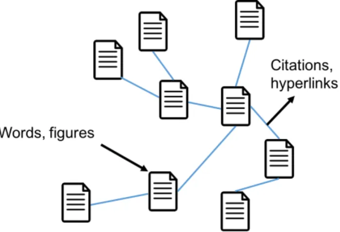
In the last part of this thesis, a much more complex relational structure is con-sidered. In particular, we aim at developing novel embedding methods for jointly modelling the linkage structure and objects’ attributes. Traditionally, link prediction task is carried out on either the linkage structure or the objects’ attributes, which does not aware of their semantic connections and is insufficient for handling the complex link prediction task. Thus, our goal in this work is to build a reliable model that can fuse both sources of information to improve the link prediction problem. The key idea of our approach is to encode both the linkage validities and the nodes neighbourhood information into embedding-based conditional probabilities. Another important aspect of our proposed algorithm is that we utilise a margin-based con-trastive training process for encoding the linkage structure, which relies on a more appropriate assumption and dramatically reduces the number of training links. In the experiments, our proposed method indeed improves the link prediction performance on three citation/hyperlink datasets, when compared with those methods relying on only the nodes’ attributes or the linkage structure, and it also achieves much better performances compared with the state-of-arts.
Declaration
The author hereby declares that this thesis is a record of work carried out in the Department of Electrical Engineering and Electronics at the University of Liverpool during the period from October 2013 to September 2017. The thesis is original in content except where otherwise indicated.
Contents
List of Figures x
List of Tables xiii
1 Introduction 1
1.1 Relational Data . . . 5
1.1.1 Representation . . . 5
1.1.2 Properties . . . 9
1.1.3 Relational Learning Tasks . . . 10
1.2 Motivation and Main Contributions . . . 12
1.3 Thesis Outline and Related Publications . . . 15
2 Generic Embedding Approaches 17 2.1 Principal Component Analysis . . . 18
2.1.1 Model Construction . . . 18
2.1.2 Multidimensional Extension . . . 19
2.1.3 Eigenvector Solution . . . 20
2.2 Laplacian Eigenmaps . . . 21
2.2.1 Model Construction . . . 21
2.2.2 Solving the Constrained Optimisation Problem . . . 22
2.3 Locality Linear Embedding . . . 24
2.3.1 Model Construction . . . 24
2.3.2 Computing the Weight Matrix . . . 25
2.3.3 Computing the Embedding Coordinates . . . 26
2.4 Stochastic Neighbour Embedding . . . 27
2.4.1 Model Construction . . . 27
2.4.2 Setting the Model Parameters . . . 28
2.5 Canonical Correlation Analysis . . . 29
2.5.1 Theoretical Foundations . . . 29
2.5.2 Multidimensional Extension . . . 31
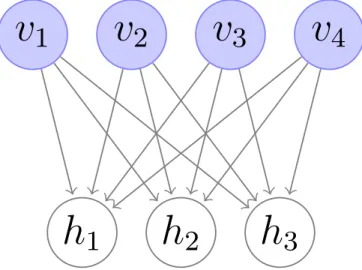
2.6 Restricted Boltzmann Machine . . . 33
2.6.1 Theoretical Foundations . . . 33
2.7 Conclusion . . . 36
3 Heterogeneous Object Co-embeddings from Relational Measurements 37 3.1 Introduction . . . 37
3.2 Related Methods . . . 39
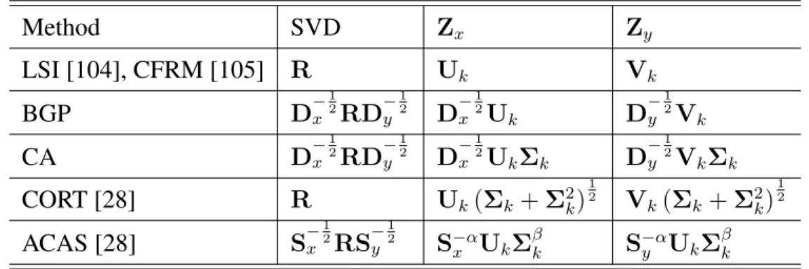
3.2.1 Co-occurrence Data Embedding . . . 40
3.2.2 Bipartite Graph Partitioning . . . 42
3.2.3 Correspondence Analysis . . . 46
3.2.4 Automatic Co-embedding with Adaptive Shaping . . . 48
3.3 The Proposed Framework . . . 50
3.3.1 Model Construction . . . 50
3.3.2 Co-Embedding Generation . . . 53
3.3.3 Multidimensional Extension . . . 56
3.3.4 Model Identification . . . 59
3.4 Experimental Analysis and Results . . . 60
3.4.1 Reconstruction of Synthetic 2D Data Points . . . 64
3.4.2 Learning Distributional Representations of Documents and Words . . . 66
3.4.3 Co-embedding Generation from Link Data . . . 72
3.4.4 Further Analysis of the Proposed Method . . . 76
3.5 Conclusion . . . 82
4 Knowledge Graph Embedding 85 4.1 Introduction . . . 85
4.2 A Brief Review . . . 88
4.3 Previous Methods . . . 89
4.3.1 Non-Translation Models . . . 90
4.3.2 Translation Methods . . . 92
4.4 The Proposed Method . . . 95
4.4.1 Model Construction . . . 95
4.4.2 Model Training . . . 97
4.4.3 Discussion . . . 98
4.4.4 Data Partition Scheme for Evaluation . . . 101
4.5 Experiments . . . 103
4.5.1 Datasets and Experimental Setup . . . 103
4.5.2 Performance Comparison . . . 105
4.6 Conclusion . . . 110
5 Link Prediction in Document Networks 112 5.1 Introduction . . . 112
5.2 Related Work . . . 115
5.2.1 Pairwise Link-LDA . . . 115
5.2.2 Relational Topic Model . . . 117
5.2.3 Communities from Edge Structure and Node Attributes . . . 118
5.2.4 Structure Preserving Metric Learning . . . 120
5.3 Proposed Formulation . . . 121
5.3.1 Encoding Link Validities as Stochastic Variables . . . 122
5.3.2 Modelling the Linkage Structure . . . 123
5.3.3 Modelling the Attributes Data . . . 124
5.3.4 Training Procedure . . . 126
5.4 Experimental Analysis and Results . . . 127
5.4.1 Mean Rank Evaluation . . . 127
5.4.2 Sensitivity Analysis of Model Parameters . . . 131
5.5 Conclusion . . . 133
6 Conclusion 135 6.1 Summary . . . 135
6.2 Future Work . . . 137
List of Figures
1.1 In a document network, each document contains its contents (such as figures, tables and text contents) as well as its linkages (or citations) to other documents. . . 9
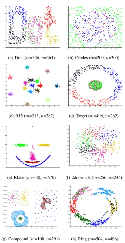
2.1 A graphical depiction of an RBM with4visible and3hidden units. 33 3.1 Original patterns of the synthetic 2D datasets. Different colours
correspond to different clusters and spatial structures. All points with the same colour are allocated either to groupX(marked by “◦”) or to groupY(marked by “+”). The cardinalitiesm=|X|andn =|Y|
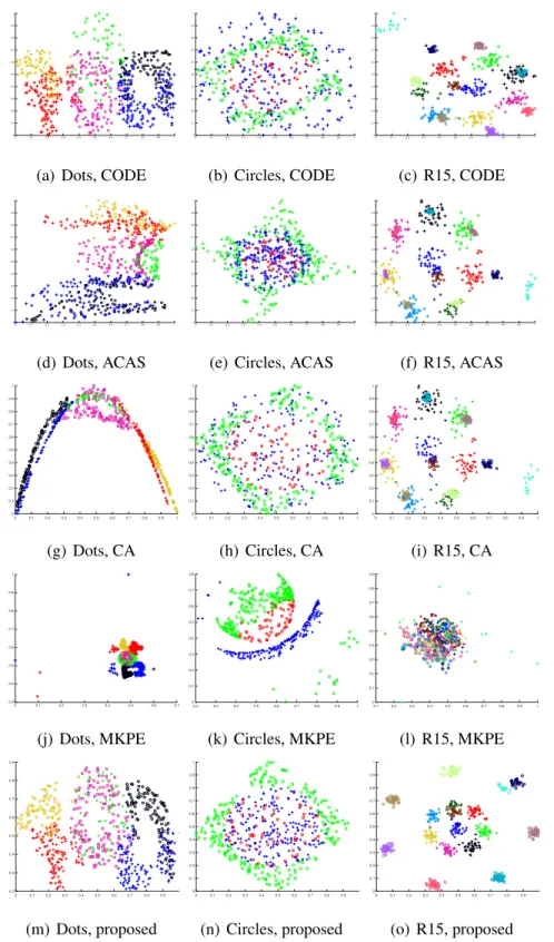
of the groups are shown for each dataset. . . 63 3.2 Co-embeddings generated by different algorithms, for the synthetic
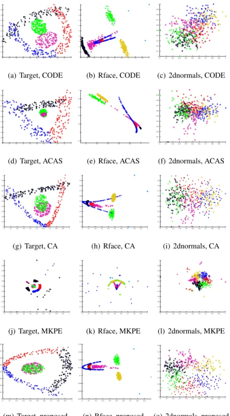
datasets of Dots, Circles and R15 displayed in Figure 3.1. Co-embedding axes are scaled within[0,1]. . . 65 3.3 Co-embeddings generated by different algorithms, for the synthetic
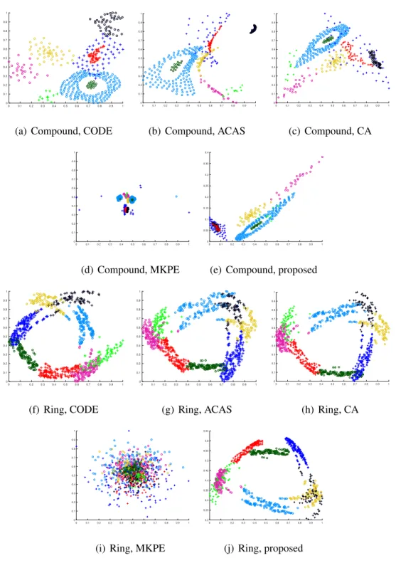
datasets of Target, Rface and 2dnormals displayed in Figure 3.1. Axes are scaled within[0,1]. . . 67 3.4 Co-embeddings generated by different algorithms, for the synthetic
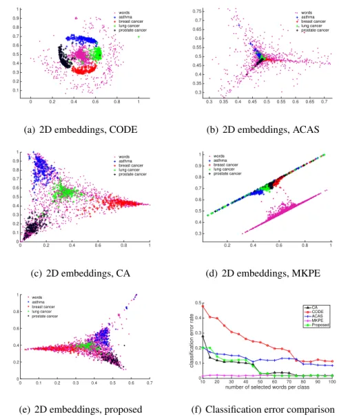
datasets compound and ring displayed in Figure 3.1. Co-embedding axes are scaled within[0,1]. . . 68 3.5 2D demonstration of co-embeddings generated for 800 clinical trials
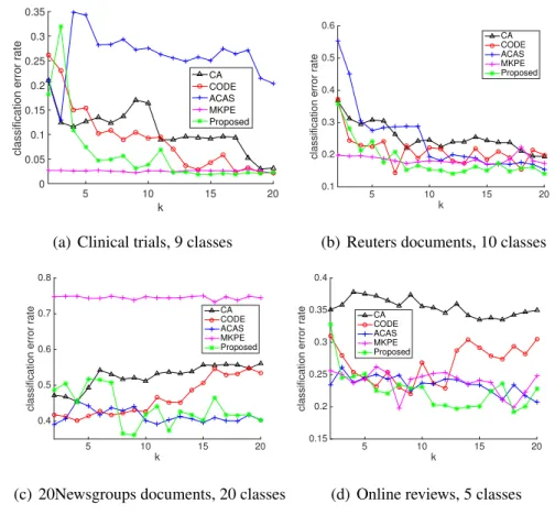
and 1,780 words belonging to four classes by different methods and their classification error comparison. Each document (marked by “+”) is a member of groupXand belongs to one of the four topics (plotted in different colour). Each member of groupY(marked by “•”) is a word object. . . 70 3.6 Comparison of the classification error rates of different algorithms,
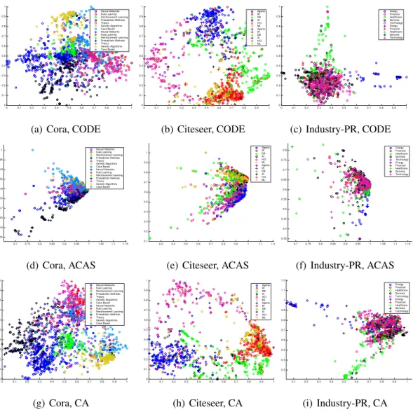
for varying the number k of the selected words that are closest to each class centre using different document collections. . . 71 3.7 2D co-embeddings generated by different algorithms, for the Cora
and Citeseer datasets. Row objects (marked by “+”) and column objects (marked by “◦”) are members of different classes plotted in different colours. . . 73
3.8 Quantitative comparison of different co-embedding algorithms in terms of the mean rank score and classification error rates using the three link datasets. . . 75 3.9 2D embeddings generated by the proposed algorithm with varying
settings of the neighbourhood control parameters kr and kcusing
the three synthetic datasets dots, compound and ring (in each corre-sponding column). . . 78 3.10 2D embeddings generated by the proposed algorithm with varying
settings of the neighbourhood control parameterskrandkcusing the:
(a-e) 4-class clinical trials, and (f-j) Citeseer dataset. . . 79 3.11 Performance comparison of the proposed algorithm under varying
settings of the neighbourhood control parameters kr and kc. (a)
Classification error rates using the whole clinical trial collection. (b,c) Classification error rate and mean rank values using the Citeseer data. The experimented settings ofkrandkcare shown in the legends.
The typical setting of kr = kc = 5 and similar local settings of
kr = kc = 10 and kr = kc = 15, as well as the worst setting of
kr =mandkc=nare also included. . . 80
3.12 Computational cost comparison of different methods for increasing number of data size (n, m) and embedding dimension (k). The incremental integer values on x-axis mark the different settings of data size. . . 82 4.1 Real world facts stored as a KG, of which the triplet form is
ex-pressed as (head_entity, link, tail_entity), i.e. (chris_noth, starred_in,
sex_and_the_city),sex_and_the_city, is_a, tv_show). . . 86
4.2 Illustration of the performance change of TransPES against each of its three algorithm parameters (k, λ2, γ) in terms of the raw and filtered
mean rank, also the filtered hits@10 measurements, evaluated using validation and test sets marked as “valid" and “test" respectively in each plot. . . 107
5.1 Graphical representation of the Pairwise Link-LDA model. This plate only shows the generation of one directional link yd,d0 from
documentdto documentd0. . . 116 5.2 Graphical representation of the RTM model. This plate only shows
the generation of one undirected linkyd,d0 between documentdand
5.3 Illustration of the performance with respect to different settings of the embedding dimensionality k, surrogate margin parameter γ∗ = γ ×(sample size)and the regularisation parameterλon the three used datasets. In each figure, two parameters are fixed as the ones in Section 5.4.1, the performances correspond to the different setting of the third parameter are displayed. . . 132
List of Tables
3.1 A summary of different co-embeddings methods, the second column shows the matrix on which SVD is performed, and the co-embedding computations are listed in the third and fourth columns. . . 49
4.1 Different embedding models with the associated energy function and parameters specified. Bothkanddare the dimensions of embedding space, we assumekto be the final reduction dimensionality (k < d in general). ׯ3 denotes then-mode vector-tensor product along the
3rd mode. . . 91 4.2 Examples of reverse triplets. . . 102 4.3 Statistics of datasets. . . 104 4.4 Performance comparison for WN18 and FB15k datasets. The best
performance is highlighted in bold, and second best underlined. . . . 106 4.5 Detailed evaluation on FB15k. Best performance is highlighted in
bold, and second best underlined. . . 109 4.6 Link prediction comparison between TransE and TransPES over the
reciprocal, reverse and other triplets in the test set of FB15k data. . . 109 5.1 Summary statistics for the three datasets after processing. . . 127 5.2 Mean ranks of different algorithms for predicting links based on
both the attribute representations and the existing linkages. The best performance is highlighted in bold, and second best underlined. . . . 130 5.3 Mean ranks of different algorithms for held out documents. The best
Abbreviations
SRL Statistical Relational Learning. 3, 4 MCMC Markov Chain Monte Carlo. 4
LLE Locality Linear Embedding. 12, 24, 27, 36 KG Knowledge Graph. 14, 16, 85–89, 101, 110, 136 LE Laplacian Eigenmaps. 17, 21, 22, 36, 50
SNE Stochastic Neighbour Embedding. 17, 27, 28, 36 PCA Principal Component Analysis. 18–20, 36 CCA Canonical Correlation Analysis. 29–32, 36, 38 RBM Restricted Boltzmann Machine. 33–36
CA Correspondence Analysis. 38, 46–48, 60, 64, 69, 76, 77, 82
CODE Co-occurrence Data Embedding. 38, 40–42, 60, 64, 69, 76, 77, 82
ACAS Automatic Co-embedding with Adaptive Shaping. 38, 48–50, 60, 64, 69, 76, 77, 82, 136
PSD Positive Semi-Definite. 41, 42, 120 BGP Bipartite Graph Partitioning. 42–45, 49
MKPE Multiple Kernel Preserving Embedding. 60, 64, 66, 69, 76, 77, 82 TransPES Translating on Pairwise Entity Space. 88, 105, 110
SE Structured Embedding. 89, 90
LFM Latent Factor Model. 89, 92 SME Semantic Matching Energy. 89, 92
LDA Latent Dirichlet Allocation. 115, 136, 138
MMSB Mixed Membership Stochastic Block. 115, 117 RTM Relational Topic Model. 117, 118, 129, 131
CESNA Communities from Edge Structure and Node Attributes. 118, 129, 131 SPML Structure Preserving Metric Learning. 120, 121, 129, 131
SPE Structure Preserving Embedding. 120, 121 SDP Semi-Definite Programming. 121
Chapter 1
Introduction
In many information domains, an object is usually characterised by a continuous or discrete feature vector of attributes, e.g., a scientific paper can be represented by its contextual words, references and key words; genes and gene products are often characterised at multiple levels including mRNA expression levels, protein abundance levels, cellular location and other factors; an image is characterised by its pixel intensity of colour channels or its associated text descriptions. With the attribute representations (or propositional representations [1]), traditional machine learning algorithms are concerned with learning a mapping from the input feature vectors to an output of interest, which may correspond to class labels, regression target values, clustering identifiers or intrinsic latent representations. Although many such attributes-oriented algorithms can generalise well (e.g., predict, learn the concepts) to new data from the problem domain, the rich information regarding the relationships between objects or attributes is ignored, which should be useful for uncovering, understanding, and exploiting the intrinsic properties of the data. For example, in natural language processing, the references for scientific papers are created with different types of motivations (e.g., relevant works, empirical findings, background reading), which are usually relevant to the central theme of the citing paper; in biology, the activation of a subset of genes or the protein domain interactions in a cellular compartment may correspond to a common functional process (e.g., cellular differentiation processes, protein synthesis processes, protein-protein interactions); in image processing and analysis, the visual contents in a scene are usually semantically
Introduction 2 interacted, and the salient interactions in the image are interpreted by its associated textual descriptions.
Indeed, learning to reason on the relationships is of vital importance in the physi-cal and natural world. In physics, any of the four fundamental forces – gravitational, electromagnetic, strong, and weak – are considered as the ways that individual parti-cles interact with each other [2]. It turns out that all physical aspects of the universe can be fully explained and linked together by these basic interactions. In a natural world, the organisms and their physical environment are linked together through processes of energy transfer and nutrient cycles. Understanding the vital connections between plants and animals and the world around them can provide us information about the benefits of ecosystems, manage our natural resources, and protect human health [3]. Moreover, the relational data can be very helpful for understanding and handling human generated big data, allowing one to infer and exploit latent properties, classes and structures about objects. Taking the email network as an example, which embodies the relations of sending and replying to messages, we are interested in exploiting the relational aspects of this data to uncover various latent properties (e.g., roles, communities and preferences) of the instances.1 It can be noted that people who frequently receive messages containing relational types of assistant requests like photocopying, hotel bookings and meeting room arrangements are identified to have the latent role "administrative assistant". As another example, real world knowl-edge can be stored in a relational database, e.g., Semantic Web, Linked-Cloud and knowledge bases, and an inference engine can reason about the existing knowledge in the data to deduce new facts or highlight inconsistencies. Recently, the content of relational data is growing rapidly with the development of various areas such as web mining, bioinformatics, social network analysis and marketing.
Developing effective and reliable methods to deal with such unreliable, complex, and large-scale relational structure has been considered as one of the greatest chal-lenges for today’s machine learning. The first difficulty is that most relations are inherently vague and ambiguous. For example, in a movie rating database, viewers rate a movie via a score, of which the quantity is not precise at all for measuring
Introduction 3 their "degree" of inclination, but rather intuitive. And even if different people like the same movie, the reasons behind their motivations are usually very different: i.e., Jo may like Top Gun because she loves 80s action movies, while Felix likes Top Gun because he likes movies with Kenny Loggins soundtracks. So the fact that both viewers watched and rated the movie highly does not necessarily mean they will value the same set of other movies with high probabilities. On the other hand, most relational data are incomplete, noisy and including false information, a problem that is being aggravated due to the increasing usage of automatic information extraction techniques. Thus, a relational learning model also needs to be considered for improv-ing the quality of a relational database, such as predictimprov-ing unknown relationships, correcting existing relations, and detecting duplicate objects.
A worth mentioning field addressing the learning and inference from the uncertain and complex relational data is calledStatistical Relational Learning (SRL), which relies on a variety of statistical models that target relational learning tasks. Early SRL focuses on relational graphical models [1], which can be divided into two categories: a)logic-based (i.e., rule-based) models andb) frame-based (i.e., object-oriented) models. The logic-based models build upon combining the traditional inductive
logic programming[4] methods for representing knowledge in the first-logic setting
and graphical models for supporting probabilistic reasoning, i.e., Bayesian logic programs [5], stochastic logic programs [6] and Markov logic networks [7]. Frame-based models extend the traditional graphical models, such as Bayesian networks and Markov networks, avoiding their underlying i.i.d. assumption by incorporating the relational database models. For example, probability relational models [8, 9] define a probability model based on a relational database. The directed acyclic probability entity relationship model [10] adapts Bayesian analysis to entity-relationship database representation [11]. The relational Markov network [12] and relational dependency networks [13] are the relational extensions to the Markov networks. In these relational graphical models, objects and attributes are encoded by random variables and the statistical dependencies between these variables are either built from prior knowledge or inferred from the data automatically. To enable effective training, a variety of approximate inference methods has been utilised, such as variational inference,
Introduction 4 loopy belief propagation and Markov Chain Monte Carlo (MCMC) methods [14–16]. However, these models still remain highly expensive to train since they require a large number of statistical dependencies to build the dependency structure to link together the objects. If the required dependency structure is unknown, it has to be inferred automatically from the data, which is often very complex and time-consuming [17–19]. Hence, it is impractical to apply these relational graphical models to large-scale relational learning problems.
For effectively handling the relational structure, recent developments in SRL have devoted to latent variable models [20–22]. Unlike the relational graphical model, the statistical dependencies in these models are not solely explained using variables that have been observed in the data. Latent variable models assume that there are hidden causes for the observable data and model the probability of a particular relationship via either random generation processes or simple operations on some latent variables, i.e., variables that are not directly observed but are rather inferred from other observed variables. Simultaneously, the dependency structure is defined through only a small number of latent variables (e.g., group memberships, latent roles ). As a result, such models do not suffer a loss of expressiveness and avoid the time-consuming structure learning that is necessary for the functioning of the previous models.
Embedding methods are latent variable models in which each entity is represented as a point in the latent space (e.g., Euclidean space), and a relation is modelled as the mathematical operation between these entity vectors. In multi-relational database [23, 24], they further assign each type of relationships to an operation that is characterised by vectors, matrices or tensors. These approaches seek a balance between the expressiveness and the complexity of their models and have been successfully applied to a range of relational learning problems, especially for the very large scale multi-relational data. Moreover, it has been shown that some latent vectors learned by these models coincidentally relate to the semantic relationships between entities. For an example, in text embedding [25], if you take the embedding vector of Paris, subtract the embedding vector of France, and add the embedding vector of Germany, the resulting embedding vector will be close to the embedding vector of Berlin.
1.1 Relational Data 5 In the following content of this chapter, we first provide a formal definition of relational data with its categorisations, properties and relevant relational learning tasks. Then we state our motivations and summarise the main contributions of this thesis. At last, we briefly describe how our thesis is organised.
1.1
Relational Data
1.1.1
Representation
All sorts of real world systems can be represented in a relational structured format in which the instances are linked (i.e., related) to each other. One could represent relational structure as networks (also referred to as graphs), whose nodes represent the objects and edges correspond to the connections between objects. Though the network model is insufficient for representing all relational structures (e.g., ternary relationships,n-ary relationships), it provides us a natural view of data by isolating entities and relationships. For example, the Internet is a big worldwide communica-tion network where the nodes are computers and the edges are physical (or wireless) connections between the computers. The World Wide Web is a network where the webpages are nodes and hyperlinks are edges. Other examples include social networks of acquaintances, publication networks linked by citations, transportation networks with the flow of vehicles and metabolic networks of metabolic pathways. To illustrate the subtle details, we follow the mathematical definition of relational data in this chapter, based on the entity-relationship model [11].
A relational data set contains a set of entities and relationships. An entity is a "thing" which can be distinguished from other "things". It can exist physically or logically, i.e., a specific object, event or concept is an example of an entity. We should distinguish between an entity and an entity set, where an entity set is a category that the entities belong to. In other words, an entity is an instance of a given entity set. LetEidenote theith entity set. In general, the entity sets are not mutually disjoint.
For instance, an entity in the entity set ”male-person” must also belong to the entity set ”person”. In this respect, entity set ”male-person” is a subset of the entity set ”person”.
1.1 Relational Data 6 Consider associations among entities. Ann-ary relationship setR, is a mathe-matical relation amongnentities, each taken from an entity set:
{(e1, e2, . . . , en)|e1 ∈E1∧. . .∧en∈En} (1.1.1)
and we refer to a singlen-tuple(e1, e2, . . . , en)as a relationship2between the entities
e1, e2, . . . , en. Note that a relation can exist between the same set of entities. For
example, a "marriage" is a relationship between two entities in the same entity set ”person”. And there may exist heterogeneous relations among the same set of entities.
For example, besides the "friendship" relation, there may also exist an "officemate" relation between employees.
For ann-ary relationR, its characteristic mapping function is defined accordingly, as
φR : E1×E2×. . .×En7→ {0,1} (1.1.2)
where×denote the Cartesian product of sets. Following this definitions, the boolean-valued characteristic functionφRgives true if and only if a particular relationship exists. In other cases, φR can map each relationship to a real number, indicating the strength of the associated linkage. There are also observations or measurements information about the relationship or entity, which are usually expressed by a feature vector of attributes. For example, a person can be described by different attributes, such as inch, colour and height. Optionally, the relevant category information of entities can also be provided as attributes in a relational data.
In this thesis, we are only interested in binary relations, which only occur between two entity sets. Therefore, the characteristic mapping values of any particular relation for all possible entity pairs can be represented by a matrix (we referred to it as a characteristic matrix). For example, the ”friendship” relation between employees can be represented by a matrix, where theijth entry indicates whether employeeiis a friend of employeejor not. We denote the characteristic matrix for thekth relation
RkasAk, in the context of a single relationR, we overload it by a simple matrixA.
In general, a relational data can be very complex, e.g., including multiple relation sets and entity sets, and each element of these sets may be described by different
2We distinguish "a relationship" and "a relation" in this thesis. A relationship refers to ann-ary
1.1 Relational Data 7 attribute sets. Simultaneously handling all sorts of different information in a relational data is a very challenge task since there may have multiple levels of uncertainty about the data, i.e., uncertainty about the number of attributes, attribute’s type, and the identity of an object as well as relationship membership, attribute and type. Moreover, collecting a complete description of every entity and relationship in the data is generally impractical. It is thus necessary and important to study only the partially available information within a relational database. Therefore, relational data is divided into simpler data formats, each of which is covered by different subfields of relational learning. We address some important categories of the relational data as following:
• Undirected graph: An undirected relation is symmetric in that its characteris-tic matrix satisfiesA(i, j) = A(j, i)for any entity pairiandj. For example, a "marriage" relation is an undirected relation as if personiis married to person j, personj is also married to personi. Similarity or dissimilarity information can be viewed as undirected relations, given objects characterised by such information, Multidimensional Scaling [26] and its variants attempt to model such information as distances among points in a geometric space.
• Directed graph: A direct relation is asymmetric and it typically has an asym-metric characteristic matrixAfor describing directional relationships in a data set. Examples include paper citation relations, hyperlink relations between webpages and sending/replying relations in an email network. The directed net-work data is usually served as the base information for more complex relational data, it is thus very important to uncover the interdependency information between observations in this simple network. For this type of data, a mixed-membership model [22] is able to capture the multiple roles that objects exhibit in interactions with others in a friendship network and a protein interaction data.
• Bipartite graph: The relational measurements in a bipartite network are between two groups of heterogeneous objects. It can be either undirected or directed — such as co-occurrence rates of articles and words in text data or item
1.1 Relational Data 8 ratings given by users in a recommendation system. Commonly co-occurrence data learning approaches are topic modelling [27] and joint embeddings [28]. Collaborative filtering [29, 30] is a field for processing the preference (rating) data that is collected from many users. In general, the propositional data can also be generalised to bipartite relations if we treat the attributes as another set of entities.
• Multi-relational data: Relational data typically consists of several types of relations among entities. Handling multi-relations is essential for identifying valid, novel, useful, and understandable patterns from large datasets. Recently, a large number of works regarding multi-relational data learning have been proposed (see [31] for a review), based on learning the semantic embeddings of the structured text.
• Document Network: By document network, we refer to the kind of relational data where the objects are described by a single type of relations associated with objects’ feature representations. Specifically, the attributes for represent-ing objects are fixed and defined in the same homogeneous set. As such, the feature vectors for all the objects have the same dimensionality. The fusion of these two sources of information has proven to enhance the models’ ability for classification [32] and link prediction along with improved latent represen-tations [33]. A small example of the document network data is provided in Figure. 1.1.
There are other types of relational data with more components and more complex dependency structure. For examples, [34, 35] included the relations’ associated text to better identify the group memberships in a network. In [36, 37], the object labels are utilised to derive a combined classification of the network data. Also, different dependency patterns have been explored such as collaborations in co-authorship networks, which are jointly modelled with the co-occurrence terms in a text body to refine the discovery of abstract "topics" [38].
1.1 Relational Data 9
Figure 1.1: In a document network, each document contains its contents (such as figures, tables and text contents) as well as its linkages (or citations) to other documents.
.
1.1.2
Properties
Unlike the propositional data representations, the objects in a relational structure are inter-linked to each other. Without prior knowledge, such very complex interde-pendence structures are very difficult to exploit. However, two primary patterns are shown to prevail and structure the ties of many network data, namely, homophily and stochastic equivalence, which should be useful for developing relational learning algorithms. We describe these two patterns and illustrate how they can be exploited by relational learning methods as below.
• Homophily: The principle of homophily indicates that the relationships be-tween similar objects are stronger than the relationships among dissimilar objects, which is also well-known as in the proverb "birds of a feather flock together". For example, people tend to make friends with regards to similar interests, ages, and analogous many other characteristics. It has been discov-ered in a large-scale of literature from the analysis of social networks [39]. Homophily provides the predictive patterns for relational data, such as pre-dicting the religion of a person from the religions of his or her friends in a social network. In designing relational learning algorithms, the homophily is
1.1 Relational Data 10 captured by either the similarity of observable/hidden object representations or the connectivity patterns of nodes in a network.
• Stochastic Equivalence: Sometimes, the individual object may exhibit its relationships to other objects that are characterised from thecategory
member-shipsthey belong to. All objects of the same group have similar relationships
to objects of other groups. This property is referred to as stochastic equivalence in network analysis, where objects’ relationships are explained via relation-ships between their associated group memberrelation-ships. Analysis of stochastic equivalence in relational data can be very helpful for predicting unknown relationships between entities for which the memberships of these entities are known. In relational learning models, this feature is either explicitly captured by assigning latent classes or roles to entities in relational data or implicitly conveyed through the clusters/locations of the entities’ latent representations.
1.1.3
Relational Learning Tasks
Various tasks can be brought for relational data learning, which are listed as follows:
• Constructing Latent Representation: Inferring the latent representations from the observed relational structure is a fundamentally important aspect in many disciplines, including economics, medicine, bioinformatics, natural language processing, management and social sciences. It serves to reduce the dimensionality of the data and can help us to understand the observed data by revealing its underlying concepts, i.e., sometimes latent variables correspond to aspects of physical reality which could in principle be measured or correspond to abstract concepts, like categories, functionalities and hidden states. In particular, embedding objects, relations, or both in a two or three dimensional geometric space allows us to gain a quick and intuitive summary of the data.
• Link Prediction: Link prediction concerns about learning the boolean-valued characteristic functionφRfor determining the existence of certain relations. It
1.1 Relational Data 11 require the relational learning algorithms to understand the observed data based on entity attributes, relationships, and other information so that they can be used to predict the likelihood of novel associations between entities. Moreover, it has been shown in [33] that their model can even predict the existence of the words given only the links to existing articles of an new one. Alternatively, the link prediction problem has been transformed into an entity ranking task by many relational learning methods [40, 41], which ranks the objects to a query object according to their relatedness. Link prediction is central to almost all types of relational data.
• Collective Classification/ Clustering: Classifying or labelling for objects is a very important step in many application domains. These tasks are typically carried out on each object independently in standard classification/clustering setting, without considering the underlying relations between objects. While relations undoubtedly provide valuable information for classification or clus-tering, i.e., homophily in race and ethnicity naturally creates strong clustering patterns in our social network. Thus, relational learning approaches have an advantage over traditional approaches since they can improve the classification accuracy or clustering quality by including the relevant relational structure information. Numerous approaches [12, 36, 42–44] have brought clustering and classification into a relational setting, and have been shown to improve the learning results significantly.
• Object Identification: object identification is the problem of assigning an object instance with a unique, unchanging identity. It is also known as record linkage [45], entity resolution [46], instance matching [47] and data deduplica-tion [48] in other naming convendeduplica-tions. Object identificadeduplica-tion clearly has many applications. For example, in the context of word sense disambiguation, there are eight senses of ”bass” in the large lexical database WordNet [49]. Given this word in a text, object identification is find the correct choice of meaning for it in that particular context. In the database domain, object identification is required when sharing data and resources within and across organisations, as it
1.2 Motivation and Main Contributions 12 may be the case due to their differences in record shape, storage location, or curator style or preference. It is undeniable that entities are distinguishable via their patterns of connections for the reason that identical entities are expected to exhibit the same pattern of relations. Thus, object identification is made collectively by integrating various information in the relational learning setting, which has been researched in various data domains [50–53].
1.2
Motivation and Main Contributions
Methods for the generation of embeddings or pattern representations of data objects in low-dimensional spaces have been widely studied in conventional machine learning. Given the objects characterised by the feature vectors of attributes, nu-merous dimensionality reduction approaches [54–57] can be employed to learn the low-dimensional representation of these objects. Over the years, variants of these classical methods have been developed towards the ability to capture and analyse the structure and latent characteristics of larger and more complex datasets. For example, the classical dimensionality reduction method Locality Linear Embedding (LLE) [58] has been extended by [59] to process multiclass data, versions of dis-criminant embedding generation [60, 61], and projection methods are developed for processing multimodal data [62].
Embedding approaches have also been used for analysing various types of re-lational data, such as Multidimensional Scaling [26] for preserving pairwise dis-tances of the original patterns in the low-dimensional space, joint embedding meth-ods [63, 64] for heterogeneous bipartite data and many tensor factorisation [65–67] or energy-based learning models [23, 24, 68, 69] for encoding the multi-relational data into embedded points. Indeed, learning the representations of objects and relations in a low dimensional space gives us an easy and flexible way for implementing various relational learning tasks. In link prediction, link validities can be converted into mathematical operations between these latent vector representations; classification or clustering is simply conducted on the embedded points based on their pairwise neighbourhood relationships; the likelihood that two entities are identical is derived
1.2 Motivation and Main Contributions 13 from whether they are close enough in the latent embedding space.
Hence, embedding approaches provide an alternative way to solve the relational learning tasks. One promising advantage for embedding methods compared with aforementioned statistical models (e.g., relational graphical models, probabilistic latent variable models) is that the optimisation of such methods can be delivered efficiently and explicitly through either matrix decomposition or gradient-based methods. In comparison, exact learning and inference are computationally intractable in those statistical probability models for big data that they have to utilise various approximate inference methods for achieving a reasonable computation time, which comes at a cost in terms of the model stability and accuracy. In practical, relational data may correspond to massive volumes of relations that it is prohibitive to apply those expensive inference models for processing them. Therefore, it is necessary to develop novel and efficient embedding algorithms for processing large-scale relational datasets.
In this thesis, we take the embedding approaches for handling three different relational data types — bipartite graph, multi-relational data and document network (see Section 1.1.1). Accordingly, three new models are developed for processing each data type and these models are briefly introduced as follows:
• Heterogeneous Object Co-Embeddings: In Chapter 3, we examine the prob-lem of generating co-embeddings or pattern representations from two different types of objects within a joint common space of controlled dimensionality, where the only available information is assumed to be a set of pairwise rela-tions or similarities between instances of the two groups (it is thus a weighted bipartite graph). We propose a new method that models the embedding of each object type symmetrically to the other type, subject to flexible scale constraints and weighting parameters. The embedding generation relies on an efficient optimisation despatched using matrix decomposition, that is also extended to support multidimensional co-embeddings. We also propose a scheme of heuris-tically reducing the parameters of the model, and a simple way of measuring the conformity between the original object relations and the ones re-estimated from the co-embeddings, in order to achieve model selection by identifying
1.2 Motivation and Main Contributions 14 the optimal model parameters with a simple search procedure.
• Knowledge Graph Embedding: In Chapter 4, we consider to model the Knowledge Graph (KG) [70], which is a particular type of multi-relational data. A KG stores information in a graph structured format, such as a directed graph whose nodes (entities) represent the objects and edges (links) correspond to the relation types between objects. It has become a very important resource to sup-port many AI related applications, i.e., word-sense disambiguation [71] [72], search engine [73] [74], question answering [75]. Given that most KGs are noisy and far from being complete, KG analysis and completion is required to establish the likely truth of new facts and correct unlikely ones based on the existing data within the KG. An effective way for tackling this is through translation techniques which encode entities and links with hidden represen-tations in embedding spaces. We aim at improving the existing translation techniques by taking into account the multiple facets of the different patterns and behaviours of each relation type. By considering relational representations to be dependent on the entities they relate, the multi-modality of the relation type over different entities is automatically and effectively formulated as a projection matrix over the space spanned by the entity vectors. A new test data partition scheme is also proposed to offer a better understanding of the behaviour of a link prediction model.
• Link Prediction in Document Network Data: In Chapter 5, we deal with the very imbalanced document network data. In the proposed approach, we encode both the linkage validities and the nodes neighbourhood information into embedding-based conditional probabilities. And the conformity between the document network and the embedding-based conditional probabilities are trained by combining two objective functions, one is a contrastive margin-based criterion for aligning the conditional probability distribution with the network structure, the other is a Kullback-Leibler divergence measuring the mismatch between the attribute representation distribution and the embedding data distribution. By combining the information of a linkage network and
1.3 Thesis Outline and Related Publications 15 nodes’ attributes, our proposed method not only improves the link prediction performance over methods using purely the nodes’ attribute data or the linkage network data, but also gives good predictive performance when only the nodes’ attribute data is provided.
1.3
Thesis Outline and Related Publications
We organise the thesis as follows:
CH A P T E R 2 deals with the preliminaries by introducing various generic embed-ding approaches for dimensionality reduction. The chosen methods studied in this chapter represent the basic concepts and methodologies in this area. And in fact, most existing works in relational data learning are largely based on recognising some of these ideas and create novel extensions to them.
CH A P T E R 3 presents a co-embeddings generation model for the analysis of arbi-trary relational information between heterogeneous objects (e.g., co-occurrence rates between documents and terms). This model is highly efficient due to simple matrix decomposition and a small set of parameters. The capabilities of the proposed model are demonstrated for use in various machine learning tasks, and are compared to existing algorithms with multiple synthetic and real-world datasets from the text mining domain.
CH A P T E R 4 introduces an embedding model specifically for multi-relational data analysis in the text domain. It is based on the hypothesis that the relationships of the same type in a multi-relational graph should possess distinct but related representations when associate with different node pairs. To reflect this hy-pothesis, we encode every relationship as a translation vector between entities, and relate every relationship vector to their associated relation label via simple projection operators in the modelling. Our model requires only a minimal parameterisation and provides a better model interpretability. Performance comparison with the state-of-art relational learning algorithms and in-depth
1.3 Thesis Outline and Related Publications 16 analysis of the algorithm It superiority is demonstrated in various performance comparisons and deep analysis on two large KGs.
CH A P T E R 5 studies the document network data. We propose an embedding-based method that encodes both the linkage network and the nodes’ attribute representations into conditional probabilities. This model utilises a pairwise margin-based criterion that better respect the linkage structure and is consis-tently shown to achieve the best link prediction performance among all the comparing methods.
CH A P T E R 6 concludes the whole thesis. We underline the contribution of this thesis, recapture the key ideas, and propose several potential directions for future research.
The publications produced from this research work are listed as follows:
• Wu, Y., Mu, T., Liatsis, P. and Goulermas, J.Y., 2017. Computation of het-erogeneous object co-embeddings from relational measurements. Pattern
Recognition, 65, pp.146-163.
• Wu, Y., Mu, T. and Goulermas, J.Y., 2017. Translating on pairwise entity space for knowledge graph embedding.Neurocomputing, 260, pp. 411-419.
Chapter 2
Generic Embedding Approaches
Embedding approaches give each datapoint a location in a lower dimensional space while preserving as much of the significant structure of the original high-dimensional data as possible. In this chapter, we explore the generic embedding models since they are building blocks for developing more complicated methods or to process more complex data structure. Almost all the relational learning algorithms are implicitly developed based on these generic embedding methods. For example, the methods present in Chapter 3 and Chapter 5 in this thesis are partly dependent on the ideas of the two generic embedding methods in this chapter, i.e., Laplacian Eigenmaps (LE) [56] and Stochastic Neighbour Embedding (SNE) [76]. Hence, it is of vital importance to investigate these generic methods in great detail.
Notations: From Section 2.1 to Section 2.4, we are given a set of datapoints (samples) {xi}ni=1 of dimension d, where xi = [xi1, . . . , xid]>, the goal of these
dimensionality reduction methods is to generate a set of embeddings{zi}ni=1 of
di-mensionk(kd), wherezi = [zi1, zi2, . . . , zik]>so that the embedding datapoints
in matrixZ = [zij]capture as much intrinsic structure of the original datapoint matrix
X = [xij]as possible. For those methods in Section 2.5 and Section 2.6, different
2.1 Principal Component Analysis 18
2.1
Principal Component Analysis
2.1.1
Model Construction
Principal Component Analysis (PCA) [77] is a linear method that seeks a pro-jection from high dimensional data onto a lower dimensional space, such that the variance of the projected data is maximised. To begin with, we shall consider the simpler case of projecting the high dimensional data onto a line first. Letwbe the unit vector in the direction of this line. Each data pointxiis projected onto this line
with the location given by the scalarw>xi. Note that the mean of the projected data
points is calculated by 1 n n X i=1 w>xi =w>x¯, (2.1.1)
where theddimensional vectorx¯ = n1 Pn
i=1xiis the sample set mean.
So the variance of the projected data is given by
1 n n X i=1 (w>xi−w>x¯)2 = 1 n n X i=1 w>(xi−x¯)(xi−x¯)>w =w> 1 n(X− 1 n1n×nX) > (X− 1 n1n×nX) w =w>Sw, (2.1.2)
whereSis the empirical sample covariance matrix defined by
S = 1 n(X− 1 n1n×nX) > (X− 1 n1n×nX). (2.1.3) Thus, the projected variance along the direction onw is given byw>Sw. To maximise it with regards to the projection vectorw, we are aware of the normalisation constraintw>w = 1. So the Lagrangian function for this constrained optimisation problem is defined as
L(w, λ1) = w>Sw+λ1(w>w−1) (2.1.4)
By setting the derivative with respect towequal to zero, we have
2.1 Principal Component Analysis 19 Thus, all the stationary points(λ1,w)for this optimisation problem are
eigen-value and eigenvector pairs of the covariance matrixS. The associated maximal quantity of the variance is
w>Sw=w>λ1w=λ1, (2.1.6)
so the variance will be maximised ifwequals to the eigenvector corresponding to the largest eigenvalueλ1, of the covariance matrixS. This eigenvector is known as
the first principal component.
2.1.2
Multidimensional Extension
In the above section, PCA only considers projecting data onto a one-dimensional space while preserves as much data variance as possible. Now, suppose the data sample is projected onto akdimensional subspace, and assume that the columns of
Wk= [w1, . . . ,wk]forms an orthogonal basis for this subspace. This indicates that
W>kWk =Ik, (2.1.7)
whereIkis the identity matrix of sizek.
Similar to the above section, PCA maximises a "projected variance" onto this space which is defined as the sum of variances in each axis. As seen from Eq. (2.1.2), it is given by
k
X
i=1
w>i Swi = Tr(Wk>SWk). (2.1.8)
Thus, thekdimensional linear space is found by solving the following optimisa-tion problem
argmax
W>kWk=Ik,
Wk∈Rn×k
Tr(W>kSWk) (2.1.9)
Notice that whenk =n, we haveTr(Wk>SWk) = Tr(SWkW>k) = Tr(S), it
indicates that the total variance of the data is invariant with respect to any other orthogonal basis.
2.1 Principal Component Analysis 20
2.1.3
Eigenvector Solution
The trace optimisation problem in Eq. (2.1.9) is a well-known result of linear algebra that will be exploited repeatedly in this thesis. An overview of a variety of such problems is discussed and solved in [78]. We give an effective proof to derive the eigenvalue solution for this problem in this section.
Firstly, the empirical variance matrixScan be decomposed as
S=UΛU>, (2.1.10)
whereΛ= Diag(λ1, . . . , λn)is a diagonal matrix whose entries are the eigenvalues
ofSandUis an orthogonal matrix containing the associated eigenvectors. Here, we assumeλqdecreases with increasing subscriptq.
LetP=U>Wk, it is easy to see that the columns ofPstill forms an orthogonal
basis for ak dimensional subspace. We can equivalently rewrite the optimisation problem Eq. (2.1.9) with respect toPas
argmax
P>P=Ik,
P∈Rn×k
Tr(P>ΛP). (2.1.11)
And for this trace quantity, we can further prove that
Tr(P>ΛP) = n X i=1 λi( k X j=1 p2ij) ≤λ1+. . .+λk. (2.1.12)
This inequality is an immediate consequence ofPn
i=1( Pk j=1p 2 ij) = Tr(P >P) = Tr(Ik) = k and Pk j=1p 2 ij =kP >e
ik22 ≤ keik22 = 1(ei is the standard basis vector
with1in theith position), where the quantity kP>eik22 has to be smaller than the
squared length ofei since it is the squared length of the projection ofei onto the
column space ofP. The equality sign holds if and only if the columns ofPand the set of standard basis vector{e1, . . . ,ek}span the same subspace. Hence,Wk =UP
is an orthonormal basis of the eigenspace associated with the firstkeigenvalues. In fact, PCA aligns each principal component with the eigenvectors. Let u1, u2, . . . ,ukbe the eigenvectors corresponding to the k largest eigenvaluesλ1, . . . , λk
2.2 Laplacian Eigenmaps 21 of S. The qth principal component is computed as the qth eigenvector uq.
Con-sequently, if we denote Uk = [u1, . . . ,uk], then the associated k dimensional
embedding is given by
Z =XUk. (2.1.13)
2.2
Laplacian Eigenmaps
2.2.1
Model Construction
LE [56] is a locality neighbourhood preserving method that constructs the lower dimensional representation based on the data neighbourhood structure. It first builds a weighted undirected graphG = (V, E)with edges connecting nearby points to each other. The weighted adjacency matrixW= [wij]of this graph should reflect
the neighbourhood relationships between data points, which is chosen either as the Heat kernel with parametert
wij = e− kxi−xjk2 4t ifkxi−xjk< ξ 0 otherwise , (2.2.1) or simply wij = ( 1 ifkxi−xjk< ξ 0 otherwise . (2.2.2)
To keep the neighbouring data points staying as close together as possible, LE chooses to minimise the following objective function
n X i=1 n X j=1 kzi−zjk22wij, (2.2.3)
under appropriate constraints. Intuitively, this objective function incurs a heavy penalty for mapping close data pointsi, jfar apart since closer points refers to larger weight value wij. Thus, minimising such an objective function tends to keep the
mapped points close when their high dimensional counterparts are close.
Let Dbe the degree matrix of the graphGwith its diagonal entries defined as the column (or row, sinceWis symmetric) sums ofW. And the Laplacian matrix
2.2 Laplacian Eigenmaps 22 isL=D−W, which is positive semi-definite. It turns out that Eq. (2.2.3) can be rewritten as n X i=1 n X j=1 kzi−zjk22wij = n X i=1 n X j=1 (zi−zj)>(zi−zj)wij = n X i zi>zi( n X j wij) + n X j zj>zj( n X i=1 wij)−2 n X i=1 n X j=1 zi>zjwij = 2Tr(Z>DZ)−2Tr(Z>WZ) = 2Tr(Z>LZ). (2.2.4)
We now minimised Eq. (2.2.4) with respect to the data embedding matrix Z. Clearly, this has to a constrained minimisation to remove the arbitrary scaling factor for the mapped points inZ. LE requiresZto beD-orthogonal
Z>DZ=I. (2.2.5)
Also, LE removes the arbitrary translation factor by centring the embedded points with weights inD
Z>D1= 0, (2.2.6)
where1isn-length the vector of ones.
Finally, the minimisation problem reduces to finding
argmin
Z>DZ=I,
Z>D1=0,Z∈
Rn×k
Tr(Z>LZ). (2.2.7)
This optimisation problem can be solved in a similar manner to that of Eq. (2.1.9).
2.2.2
Solving the Constrained Optimisation Problem
We define the normalised graph Laplacian matrix L˜ = D−12LD−1
2, it is easy
to show that this real symmetric matrix is positive semi-definite. We denote its eigendecomposition asL˜ =UΛU>withΛ= Diag(λ1, . . . , λn)the diagonal matrix
whose entries are the eigenvalues in ascending order andUis an orthogonal matrix containing the associated eigenvectors. Here, we assumeλqincreaseswith increasing
2.2 Laplacian Eigenmaps 23 subscriptq. At first, we show thatD121is an eigenvector with eigenvalue0since
˜ L(D121) = D− 1 2LD− 1 2(D 1 21) =D−12L1 =D−12(D−W)1 = 0. (2.2.8)
And it is the only eigenvector for eigenvalue 0 if we assume a connected graph G[56].
Therefore, If we substitute P=U>D12Zinto the Eq. (2.2.7), the condition of
Z>D1= 0is converted as
P>U>D121=P>e1 = 0, (2.2.9)
wheree1is a unit vector with1in the first position and we have made use of the fact
thatλ1 = 0and all eigenvectors are orthogonal to derive this. Thus, to satisfy the
conditionZ>D1= 0, we simply put the first row ofPto be all zeros. And Eq. (2.2.7) turns out to be
argmin P>P=I, P>e1=0,P∈Rn×k Tr(P>ΛP) (2.2.10) Again, we have Pn i=2( Pk j=1p 2 ij) = Tr(P >P) = Tr(I k) = k, Pkj=1p2ij =
kP>eik22 ≤ keik22 = 1,λ1 = 0, the traceTr(P>ΛP)can be rewritten as
Tr(P>ΛP) = n X i=2 λi( k X j=1 p2ij) ≥λ2+. . .+λk+1. (2.2.11)
The equality sign holds if and only if the columns of P and the set of standard basis vectors {e2, . . . ,ek+1}span the same subspace. Hence, D
1
2Z = UP is an
orthonormal basis of the eigenspace associated with the2nd to the(k+ 1)th smallest eigenvalues.
Finally, letUkbe the eigenvector matrix correspond to the2nd to the(k+ 1)th
smallest eigenvalues ofL˜, LE finds thekdimensional embedding as
Z =D−12U
2.3 Locality Linear Embedding 24
2.3
Locality Linear Embedding
2.3.1
Model Construction
LLE [79] also assumes the data are sampled from some smooth underlying manifold, it then constructs the nonlinear neighbourhood preserving mapping by approximately reconstructing the locally linear geometry of the manifold in the lower dimensional space. Providednpointsx1, . . . ,xnare well-sampled such that each
data point and its neighbours are lying on or close to a locally linear patch of the manifold. In the formulation of LLE, the geometry of these patches are characterised by minimising the following cost function
E(W) = n X i=1 kxi− n X j=1 wijxjk22, (2.3.1)
where the weight matrixW = [wij]is the linear coefficients that reconstruct each
data point from its neighbours. Two constraints are imposed onW: first, each data pointxi is reconstructed only from its neighbours,wij = 0 is enforced ifxj does
not belong to this set; second, the rows ofWmust sum to one:P
j=1wij = 1. The
second restriction ensures that the optimal weights Wto the cost functionE(W)
is invariant to rotations, rescalings, and translations of the data. Consequently, the weights in Wcan reflect the intrinsic geometric properties of the manifold rather than properties that depend on a particular frame of reference.
After obtaining the optimal W that characterises the local geometry in the original data space, LLE expects to use it to reconstruct the embedded points in a lower dimensional space. In the same way to the previous cost function, the following objective function is chosen to minimise
Φ(Z) = n X i=1 kzi− n X j=1 wijzjk22. (2.3.2)
While opposed to optimising weightswij in Eq. (2.3.1), here the weights wij are
2.3 Locality Linear Embedding 25
2.3.2
Computing the Weight Matrix
We first solve the constrained least squares problem for minimisingE(W). In fact, we can minimise each term in E(W)separately for calculating the optimal weight matrixWrow by row.
Therefore, we only need to consider a single patch with a data point x, its K nearest neighboursη1, . . . ,ηKand the reconstruction weightsw= [wj]that sum to
one. The cost for this patch is written as
ξ=kx− K X j=1 wjηjk22 =k K X j=1 wj(x−ηj)k22 = K X j=1 K X l=1 wjwl(x−ηj)>(x−ηl) =w>Cw, (2.3.3)
where we have introduced the local covariance matrixC= [cjl],
C= (x−η1)> .. . (x−η1)> h (x−η1), . . . ,(x−η1) i . (2.3.4)
From its construction, we see that this covariance matrix is symmetric and positive semidefinite.
To enforce the constraint1>w = 1(1is the vector with1in each position), the Lagrangian function is defined as
L(w, µ) = w>Cw−µ(1>w−1), (2.3.5)
whereµis the associated Lagrange multiplier. DifferentialL(w, µ)with respect toµ, we have
Cw= µ
2.3 Locality Linear Embedding 26 Thus,wcan be computed through
w= µ
2(C+αI)
−1
1, (2.3.7)
whereα >0is a regularisation term to avoid invertibility and singularity problems. The Lagrange multiplierµ= 2/1>(C+αI)−11is picked to properly normalise
w.
2.3.3
Computing the Embedding Coordinates
The embedding coordinates need to be found by minimisingΦ(Z)in Eq. (2.3.2), which reduces to finding
Φ(Z) = n X i=1 kzi− n X j=1 wijzjk22 = n X i=1 zi>zi − n X i=1 n X j=1 wijz>i zj + n X i=1 n X j=1 wijzj>zi+ n X i=1 ( n X j=1 wijzj)>( n X l=1 wilzl) = Tr Z>(I−W−W>+W>W)Z. (2.3.8) Define the n ×n matrixM = I−W−W> +W>W. Notice that the above calculation also shows thatMis positive semidefinite. And
Φ(Z) = Tr(Z>MZ). (2.3.9)
This looks very familiar since we have already dealt similar trace optimisation problem of this in Section 2.1 and Section 2.2. Proceeding as we did with LE, we add a constraint on the embedded points to remove an arbitrary scale factor
Z>Z=I, (2.3.10)
and removes the degree of arbitrary translation by requiring the datapoints to be centred on the origin
Z>1= 0, (2.3.11)
where1is defined similarly as a vector of all ones.
Using the same optimisation technique for solving the minimisation problem of Eq. (2.2.7), the embedded points are given by the eigenvector matrixUkcorrespond
2.4 Stochastic Neighbour Embedding 27 to the 2nd and (k + 1)th smallest eigenvalues of M. Formally, LLE finds the k dimensional embedding points as
Z=Uk. (2.3.12)
2.4
Stochastic Neighbour Embedding
2.4.1
Model Construction
SNE [76] is a stochastic dimensionality reduction technique that tries to place the objects in a low dimensional space so as to optimally preserve the potential neighbours of the objects. It starts by encoding the high dimensional data structure into conditional or joint probabilities. Specifically, the conditional probability,pj|i,
thatxi would pickxj as its neighbour, is defined as
pj|i =
exp (−kxi−xjk22/2σ2i)
P
l6=iexp (−kxi−xlk22/2σi2)
, pi|i = 0, (2.4.1)
where a reasonableσishould enforcepj|ito be relatively high for nearby datapoints
and low for widely separated datapoints. We will present the method for determining σi in the later section.
For the low dimensional mapping, it is possible to compute a similar conditional probability,qj|i, as qj|i = exp (−kzi−zjk22/2σ2) P l6=iexp (−kzi−zlk22/2σ2) . (2.4.2)
For simplicity, SNE does not employ different values ofσ for every datapoint in its low dimensional map and it is set to √1
2
1.
The aim of SNE is to find the low-dimensional embeddingsz1, . . . ,znto match
the corresponding distributionsqj|i andpj|i as well as possible. This is carried out
through minimising a sum of Kullback-Leibler divergence between the conditional distributionsPi ={pj|i}andQi ={qj|i}over all the datapoints:
C = n X i=1 KL(PikQi) = n X i=1 n X j=1 pj|ilog pj|i qj|i . (2.4.3)
2.4 Stochastic Neighbour Embedding 28 Notice that this cost function focuses on retaining the local structure of the data: it incurs a large cost for using distant mapped points to represent nearby datapoints (i.e., for using a smallqj|i to model a largepj|i); whereas the cost for using nearby
mapped points to represent distant datapoints is almost infinitesimal.
DifferentialCwith respect to the embedding pointzihas a surprisingly interesting
form ∂C ∂zi = 2X j (pj|i−qj|i+pi|j −qi|j)(zi−zj), (2.4.4)
where the mismatch (pj|i −qj|i+pi|j −qi|j)between the pairwise similarities of
the datapoints and mapped points can be interpreted as creating forces that repel or attractziandzj. Therefore, the minimisation problem of Eq. (2.4.3) can be solved
via gradient-based optimisation methods.
2.4.2
Setting the Model Parameters
The remaining problem is to select the parameterσi to derive a proper probability
distributionPi. Since any probability distributionPi needs to be informative to drive
the learning process, it is natural to employ entropy as a measure of the randomness of this information. Let the Shannon entropyH(Pi)to be measured in bits
H(Pi) = − n
X
j=1
pj|ilog2(pj|i). (2.4.5)
SNE searches for the value ofσithat makes the entropy of each distributionPiequals
tolog2(K), whereK is a hyperparameter set by hand.
Next,σi need to be unique for any presettingK >0. We prove this by noticing
that the entropy of the distributionPi increases monotonically with the parameter
σi. Consider a distributionP ={pj}controlled bytas a simplified version to that
distribution in Eq. (2.4.1) pj = exp(−aj/t) P kexp(−ak/t) , (2.4.6)
where the positive scalars{a1, a2, . . . an}are surrogate variables for the Euclidean
2.5 Canonical Correlation Analysis 29 Differential the Shannon entropyH(P)with respect tot, we have
∂H ∂t =− ∂hP j(pjlog2pj) i ∂t =−X j ∂(pjlog2pj) ∂pj ∂pj ∂t =−X j ∂pj ∂tlog2pj+ ln 2 ∂P jpj ∂t ( ∂P jpj t = ∂1 t = 0) =−t−2X j ajpj−( X k akpk)pj log2pj =−t−2X j ajpj−( X k akpk)pj
log2[exp(−aj/t)]−log2(
X k exp(−ak/t)) =−t−2X j ajpj−( X k akpk)pj log2[exp(−aj/t)] =t−3ln 2 X j a2jpj−( X j ajpj)2 =t−3ln 2 X j a2jpj X pj−( X j ajpj)2 ≥0. (Cauchy-Schwarz inequality)
Thus, since we have ∂Hσ(2P) ≥0, the entropyH(P)must increase monotonously with
σ.
2.5
Canonical Correlation Analysis
2.5.1
Theoretical Foundations
Canonical Correlation Analysis (CCA) [80] [81] extracts the lower dimensional representations from two sets of correlated multidimensional variables, e.g., two views of the same semantic object, such that the strong relationships between these two sets of multidimensional variables are revealed. In particular, it projects the two sets of variables onto a common semantic space, and maximises the correlations their transformed data co-ordinates.
Formally, the input to CCA is a set of high dimensional datapointsS ={(x1,y1),
. . . ,(xn,yn)}of two random variables{x,y}, where each pair of measurementsxi