This is a repository copy of
Joint interaction with context operation for collaborative
filtering
.
White Rose Research Online URL for this paper:
http://eprints.whiterose.ac.uk/140731/
Version: Accepted Version
Article:
Bai, P., Ge, Y., Liu, F. et al. (1 more author) (2019) Joint interaction with context operation
for collaborative filtering. Pattern Recognition, 88. pp. 729-738. ISSN 0031-3203
https://doi.org/10.1016/j.patcog.2018.12.003
Article available under the terms of the CC-BY-NC-ND licence
(https://creativecommons.org/licenses/by-nc-nd/4.0/).
[email protected] Reuse
This article is distributed under the terms of the Creative Commons Attribution-NonCommercial-NoDerivs (CC BY-NC-ND) licence. This licence only allows you to download this work and share it with others as long as you credit the authors, but you can’t change the article in any way or use it commercially. More
information and the full terms of the licence here: https://creativecommons.org/licenses/
Takedown
If you consider content in White Rose Research Online to be in breach of UK law, please notify us by
Joint Interaction with Context Operation for
Collaborative Filtering
Peizhen Bai, Yan Ge, Fangling Liu, Haiping Lu∗
Department of Computer Science, The University of Sheffield, 211 Portobello, Sheffield S1 4DP, United Kingdom
Abstract
In recommender systems, the classical matrix factorization model for collabo-rative filtering only considers joint interactions between users and items. In contrast, context-aware recommender systems (CARS) use contexts to improve recommendation performance. Some early CARS models treat user, item and context equally, unable to capture contextual impact accurately. More recent models perform context operations on users and items separately, leading to “double-counting” of contextual information. This paper proposes a new model, Joint Interaction with Context Operation (JICO), to integrate the joint inter-action model with the context operation model, via two layers. The joint in-teraction layer models inin-teractions between users and items via an inin-teraction tensor. The context operation layer captures contextual information via a con-textual operating tensor. We evaluate JICO on four datasets and conduct novel studies, including varying contextual influence and time split recommendation. JICO consistently outperforms competing methods, while providing many useful insights to assist further analysis.
Keywords: Recommender system, collaborative filtering, matrix factorization, context aware, joint interaction, tensor
∗Corresponding author. Address: The University of Sheffield, 211 Portobello, Sheffield, S1
4DP, United Kingdom. Tel: +44 (0) 114 222 1853. Email: [email protected]
Email addresses: [email protected](Peizhen Bai),[email protected](Yan Ge),[email protected](Fangling Liu),[email protected](Haiping Lu)
1. Introduction
Collaborative filtering (CF) is popular for recommender systems in many applications such as social networks, e-commerce, and music or movie websites [1, 2, 3, 4, 5, 6, 7]. Typically, CF recommends items to users by learning user/item similarities from existing ratings. A classical CF model is Matrix Factorization (MF) [8, 9, 10, 11], which is a latent factor model [12]. It de-composes the rating matrix into two factor matrices, representing latent factors for users and items respectively. The predicted rating rij of user i on item j
can be viewed as thejoint interaction between latent factors of useriand item
j. Another formulation of the recommender system is to view CF as a matrix completion problem [13, 14, 15, 16].
The MF model considers only twoentities (user and item) involved. In con-trast, context-aware recommender systems (CARS) aim to achieve better recom-mendation performance by taking usefulcontextinformation, such as time, loca-tion, user age, gender and occupaloca-tion, into account [17, 18, 19, 20, 21, 22, 23, 24]. For instance, time is an important factor in an e-commerce recommender sys-tem. Supposing a user bought a T-shirt in the summer, recommending a T-shirt in the winter would be inconsequential. The term “context” is broadly defined in this paper. We consider an attribute such as gender, occupation, and age as a particular context, following [25, 26, 27]. E.g. both occupation and age can change over time in real applications, such as from students to engineers, academia to industry, and getting older year by year.
Karatzoglou et al. [25] proposed a Multiverse model to generalize the MF model directly to incorporate contexts. It is based on the Higher-Order Sin-gular Value Decomposition (HOSVD) [28], a Tensor Factorization (TF) model called the Tucker Decomposition [29]. Multiverse generalizes the MF model to higher order by extending the 2-D user×item matrix with additional context dimensions into a higher-order data tensor [30], e.g., a user×item×time ten-sor. This provides good flexibility in incorporating contextual information, but its computational complexity increases exponentially with the number of
con-text variables. Instead of extending the rating matrix to a tensor, Rendle [31] developed a Factorization Machine (FM) model for context-aware recommen-dation. The FM model extends the latent factor model in MF by transforming the user-item-context rating data into real-valued feature vectors via one-hot encoding [32]. Then, it treats user-item, user-context, and item-context inter-actions as inner products of their latent factors, which can improve the rating computation to linear time. There are several more complex models developed based on FM, such as the Gaussian Process FM [33], random partition FM [27], ensemble-based FM [27] and hierarchical FM [34].
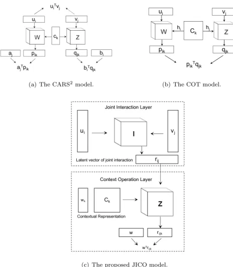
Entities (user and item) and contexts play different roles in recommender systems. However, all the CARS models above treat contexts as dimensions similar to user or item, making it difficult to interpret the relationships between entities and context, and also limiting their recommendation performance. This motivates the CARS2model [35] as depicted in Fig. 1(a). It defines the
contex-tual information in its own latent spaceck, and treats it differently from user and item latent spaces. Instead of a direct interaction between entities and con-texts, CARS2 transforms the original latent factors of users/items into a new
latent space (W/Z), which represents user/item under contexts by a 3-D con-textual operating tensor. This provides a clear interpretation of the relationship between entities and contexts.
One limitation of CARS2is that it uses one vectorc
kto represent the whole
context, which is inadequate for abundant contextual information. Liuet al. [36] proposed the Contextual Operating Tensor (COT) model to improve CARS2, as
illustrated in Fig. 1(b), motivated by the semantic compositionality and vector representationword2vec in Natural Language Processing (NLP) [37]. COT ex-tends the latent space of context representation from a vectorck to a matrixCk.
In addition, COT interprets the tensor used in CARS2as “contextual operating
tensor”, drawing analogy between the entity-context relationship with the noun-adjective relationship in NLP [38, 39, 40]. Entity is similar to a noun providing semantic information, while a context is similar to an adjective giving entities the semantic operation. Thus, COT models a context semantic operation on
Z W ck ui vj pik aj qjk bi uiTvj ajTpik biTqjk
(a) The CARS2model.
Z W Ck ui vj pik qjk hi hj pikTqjk
(b) The COT model.
ui vj JintI nt rac tnL ay r ij Z Ck wk Cexu lRep es ei Cnt tO ra t nL ay r rijk wT ijk e e f iie i
(c) The proposed JICO model.
Figure 1: Illustrations: (a) The CARS2
model, where the cubes denote 3-D contextual oper-ating tensors and the elongated rectangles denote latent factor vectors; (b) The COT model, where the squareCkis a matrix representing contextual information; (c) The proposed JICO
model with two layers, the joint interaction layer and context operation layer, which integrates the virtues of the joint interaction model in MF and the contextual operating tensor in COT.
the original latent vectors of users and items.
Although CARS2 and COT separate contexts from the latent space of
enti-ties to enhance interpretability and performance, the contexts operate on two entities, user and item separately via two contextual operating tensorsW and Z. Such separate interactions are then added (in CARS2) or multiplied (in
COT). Because the latent vectors of useruiand itemvj lie in a common latent
space, the addition and multiplication in CARS2and COT “double-count” the
impact of contextual informationck andCk. This motivates us to consider the impact of contexts on users and items jointly as in the MF models, rather than separately.
We propose a new context-aware model named as Joint Interaction with Con-text Operation (JICO) to integrate the virtues of the joint interaction model in MF and the contextual operating tensor in COT. We model the joint in-teraction between users and items as the semantic subject, i.e., the contextual information operates on the joint interaction between users and items, rather than separately. As shown in Fig. 1(c), JICO has two layers. In the first layer, an interaction operating tensorI captures the joint interaction between users {ui} and items {vj} as in MF, which is then projected to a latent space to define the joint interaction vector rij. The second layer performs the context semantic operation as in COT, where the contextual information is represented as a matrixCk.
The remainder of this paper is structured as follows. The next section intro-duces notations and related works briefly. In Section 3, we propose the JICO model and derive an algorithm based on stochastic gradient descent (SGD). In Section 4, we evaluate JICO on four popular datasets to demonstrate its superior recommendation performance over existing methods. We also study varying contextual influence, more realistic time split recommendation, result interpretation and analysis, as well as parameter sensitivity. Finally, Section 5 draws conclusions.
2. Preliminaries and Related Works 2.1. Notations
In this paper, we follow the notations in [28, 41, 42]. We denote vectors by lowercase boldface letters such asa, matrices by uppercase boldface letters such as A, and tensors by calligraphic letters such asA. AnTth-order tensorA ∈
RI1×···×IT is addressed byT indices {i
t}. Each it addresses the t-mode of A.
The mode-tproduct of a tensorA ∈RI1×I2×...×IT by a matrixU∈RJt×It is a
tensorB ∈RI1×...×It−1×Jt×It+1×...×IT, denoted as
B=A ×tU, (1)
where each entry ofBis defined as the sum of products of corresponding entries inAandU:
B(i1, ..., it−1, jt, it+1, ..., iT) =
X
it
A(i1, ..., iT)·U(jt, it). (2)
TheKronecker product (also called thetensor product) of two matricesA∈
Rr×sandB∈Rc×d results in a block matrix of sizerc×sd, which can also be
viewed as a fourth-order tensor of sizer×s×c×d:
A⊗B= a11B a12B . . . a1sB a21B a22B . . . a2sB .. . ... . .. ... ar1B ar2B . . . arsB . (3) 2.2. Matrix Factorization (MF)
In an MF model [8], the joint interaction between users and items is repre-sented with the inner product of their latent vectors. Letui,vj∈Rd represent
the latent vectors of useriand itemj. The estimated rating ˆyij is:
ˆ
yij =u⊤i vj. (4)
2.3. CARS2
CARS2 model [35] consists of three parts: the user-item, user-context and
item-context interactions. For the interaction between users and items, it follows the formula in MF, which isu⊤i vj.
For the user-context and item-context interactions, two 3rd-order tensors W ∈Rd×dp×dc andZ ∈Rd×dp×dc are given. In CARS2, the specific contextk
is denoted by a distinct vectorck∈Rdc. The impact of contextkon the useri
and itemj is formulated as:
pik=W ×1ui×3ck, (5)
qjk=Z ×1vj×3ck, (6)
where pik and qjk are dp-dimensional vectors that represent the interaction
between user/item and contexts. Then CARS2 introduces a
j, bi ∈ Rdp as
weight vectors forpik,qjk. The estimated rating ˆyijk is modeled as:
ˆ
yijk=u⊤i vj+aj⊤pik+b⊤i qjk. (7)
2.4. Contextual Operating Tensor (COT)
COT [36] extends the latent space of context representation from a distinct vectorckin CARS2to a matrixCk∈Rdc×n, wherenis the number of contexts.
The latent vectors of users and items under contexts are formulated as:
pik=W ×1ui×3(hiCk), (8)
qjk=Z ×1vj×3(hjCk), (9)
wherehi andhj are weight vectors for contextCk on useriand itemj respec-tively. The estimated rating ˆyijk is defined as:
ˆ yijk=b0+bi+bj+ n X m=1 bm,k+p⊤i,kqj,k, (10)
in whichb0,bi andbj represent the global, user and item bias respectively, and
bm,kis the bias of themth context variable. p⊤i,kqj,k is the interaction between
useriand item j under contextk, which is similar to MF.
Finally, the objective function of all three models can be expressed as below:
min L(Θ) = X
(i,j,k∈S)
(ˆyijk−yijk)2+ Ω(Θ), (11)
2.5. Double-Counting of Contextual Information
CARS2 and COT lead to “double-counting” of contextual information since
predicted rating is calculated via their product in COT and their sum in CARS2.
These two methods represent the interaction between user/item and contexts by latent vectorpikorqjk, and the contextual information is “double-counted”
via such product/sum. Our method will address this issue.
3. Proposed JICO Model
3.1. Joint Interaction between Users and Items
We propose JICO to model joint interaction as in MF and context operation as in CARS2/COT so that the contextual information can be more properly
accounted for. The JICO model has two layers. We name the first layer as the “joint interaction layer”. In this layer, we capture the joint interaction between useriand itemj. In a typical MF model, the interaction is represented by the inner product of the latent vectorsui∈Rd and vj ∈Rd, which is an effective
way to estimate ratings. However, this way of joint interaction modelling does not allow introducing the influence of contextual information. To overcome this problem, we propose to form an interaction operating tensor I ∈ Rd×dp×d to
capture the joint interaction and enable further context operation. We then define thejoint interaction vector rij as:
rij =I ×1ui×3vj. (12)
In the joint interaction layer, the interaction operating tensor I describes the common latent interaction space between users and items. With the intro-duction ofI, the interaction can now be represented as a latentvector, rather than a scalar value as in the MF model. It is intuitive that the interaction between two entities (user and item) can be evaluated from many different as-pects rather than a single value. The latent interaction vector rij can reflect
these latent aspects. Moreover, a vectorrij enables further combination with
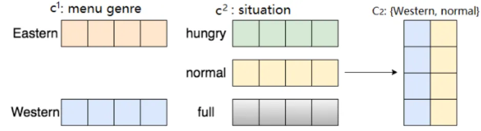
Figure 2: An example of combining two types of latent contextual information in a food rating dataset.
3.2. Contextual Information Representation
We denote contextual information set byC={C1, C2, ..., Cn}, wherenis the
number of contextual variables and each elementCirepresents a specific context
such as age, location, time, etc. Each contextual variableCi can take different
values{ci
1,ci2, ...}. Similar to the representation in COT, each specific valuecim
is represented by a latent vectorci
m∈Rdc in JICO. The vector representation
is an efficient method to describe the latent properties of contexts. As different contextual values are not always independent, they can have similar or opposite effects on the user preferences. For example, doctors and nurses may have a similar preference on certain books, but the preference of programmers may be quite different. If we just use a real value to represent the occupation, it is difficult to describe such similarity properties properly. Therefore, the latent vector provides a rich representation that can better reflect the relevance of different contextual information than a single scalar value. In this way, the whole contextual information of each rating could be individually denoted by a context combination matrix Ck = [c1m1,c
2 m2, ...,c n mn] ∈ R dc×n, where each column vector cj
mj denotes a latent vector for a specific value mj taken on
contextual variableCj. Figure 2 gives a simple example ofC k.
With the above observation, we form thecontext combination vector ck ∈
Rdc as:
ck=Ckwk, (13)
the weights of each context.
3.3. Context Operation Layer
We name the second layer of JICO as “context operation layer”. In this layer, we introduce thecontextual operating tensor Z ∈Rdp×d×dc as in COT to
take the influence of contexts into account. In the first layer, we have obtained the joint interaction vector rij of users and items. Now the tensorZ denotes
the context operation byCk onrij. Therefore, the joint interaction after the context operation can be defined as:
rijk=Z ×1rij×3ck, (14)
whererijk ∈Rd represents the joint interaction vector under contextual
infor-mationck. The estimated rating ˆyijk is then formulated as:
ˆ
yijk=w⊤rijk, (15)
wherew∈Rd is a weight vector forrijk. The JICO model has been illustrated
earlier in Fig. 1(c).
Next, we do not expect the interactionrijk can fully explain the ratings due to the existence of bias. We assume that each user or item has its own bias. For example, if a movie has a good reputation, the average rating of this movie tends to be higher and users could have different standards for rating scales. Some may be strict in evaluating a movie and tend to give low ratings but some may give high average ratings. This means that each movie or user has its own bias. To take this into accounts, we add the bias to get the following:
ˆ
yijk=bk+bi+bj+w⊤rijk, (16)
wherebkis a constant indicating the overall average rating under contexts
com-binationk,bi andbj are the bias of useriand itemj respectively. In this way,
the interaction part w⊤r
ijk can capture information from the dataset more
Algorithm 1Joint Interaction with Context Operation
Input: Training datasetS, where each real rating yijk is associated with user
i, itemj, and context combination k. Parametersη,λ1 andλ2.
Output: Updated parameters{bi},{bj},U,V, w,{Ck},{wk},I,Z
1: Initialize{bi},{bj},{ui},{vj},w,{Ck},{wk},I,Z with random values
2: Sett= 0
3: whilenot convergent do
4: η ←√1
t andt=t+ 1
5: Randomly select an instanceyijk fromS
6: yˆijk=bk+bi+bj+w⊤rijk 7: Update bi←bi−η∂b∂Li 8: Update bj←bj−η∂b∂Lj 9: Update ui←ui−η∂L∂ui 10: Update vj←vj−η∂∂Lvj 11: Update w←w−η∂L ∂w 12: Update Ck ←Ck−η∂∂LCk 13: Update wk ←wk−η∂∂Lwk 14: Update I ← I −η∂L ∂I 15: Update Z ← Z −η∂L ∂Z 16: end while
3.4. Objective Function and Parameters Inference
After introducing the JICO model, we formulate the JICO objective function to minimize using the squared error loss function:
min Θ L= X (i,j,k∈S) (ˆyijk−yijk)2 +λ1 2 (kuik 2+kv jk2+kCkk2+kwkk2+kIk2+kZk2+kwk2) +λ2 2 (kbik 2+kb jk2), (17)
where Θ ={ui,vj,Ck,wk,I,Z,w} represents the set of parameters in the
parameters. We denote the Frobenius norm of a tensorZ ∈Rdp×d×dc as kZk,
which is defined as follows: ||Z||= v u u t dp X i=1 d X j=1 dc X k=1 z2 ijk, (18)
wherezijk is the element at (i, j, k) ofZ.
The regularization terms control the magnitude of parameters to avoid over-fitting. In this paper, we use a common optimization scheme, stochastic gradient descent (SGD), to update parameters. The gradients with respect to parameters inL(Θ) can be calculated as:
∂L ∂bi = 2lijk+λ2bi, (19) ∂L ∂bj = 2lijk+λ2bj, (20) ∂L ∂Ck = 2lijk(Z ×1(I ×1u⊤i ×3v⊤j)⊤×2w⊤)⊤wk+λ1Ck, (21) ∂L ∂wk = 2lijk(Z ×1(I ×1u⊤i ×3v⊤j)⊤×2w⊤)Ck+λ1wk, (22) ∂L ∂w = 2lijkZ ×1(I ×1u ⊤ i ×3vj⊤)⊤×3(Ckwk)⊤+λ1w, (23) ∂L ∂ui = 2lijkI ×3vj⊤×2(Z ×2w⊤×3(Ckwk)⊤) +λ1ui, (24) ∂L ∂vj = 2lijkI ×1u ⊤ i ×2(Z ×2w⊤×3(Ckwk)⊤) +λ1vj, (25) ∂L ∂I = 2lijku ⊤ i ⊗(Z ×2w⊤×3(Ckwk)⊤)⊗vj+λ1I, (26) ∂L ∂Z = 2lijk(I ×1u ⊤ i ×3v⊤j)⊗w⊤⊗(Ckwk)⊤+λ1Z, (27)
wherelijk = ˆyijk−yijk.
Algorithm 1 summarizes the pseudocode for JICO. The matrices U∈RI×d
and V ∈ RJ×d are the user and item latent matrices (I/J is the number of users/items). The ith row of Udenotes the user latent vector ui and the jth row ofV denotes the item latent vectorvj. η is the learning rate. It decreases with the number of iterations increases. In each iteration, the algorithm will evaluate and update only one relevantuiandvj. To prevent gradient explosion,
the elements of initial matrices and tensors are drawn from a zero-mean uniform distribution in the range [-1
2, 1
2]. When the iteration converges, we obtain the
final parameters for estimating the rating in test data.
3.5. Computational Complexity and Model Complexity
We follow CARS2[35] and COT [36] to analyse the computational
complex-ity of JICO. To simplify the analysis, we setdp =dc =d. The computational
complexity of JICO is dominated by the computation ofU,V,I andZ, which have complexityO(d3× |S|). Therefore, the total computational complexity is
O(d3× |S|), which is similar to that for CARS2 [35] and COT [36].
The model complexity of JICO (ΓJ) and COT (ΓC) are presented as follows:
ΓJ=d×dp×d | {z } I +dp×d×dc | {z } Z +dc×n2 | {z } {Ck} +d×I | {z } {ui} +d×J | {z } {vj} +d ↓ w + n ↓ {w k} 2+ I ↓ {bi} + J ↓ {bj} , (28) ΓC =d×dp×dc | {z } W +d×dp×dc | {z } Z +dc×n | {z } {Ck} +d×I | {z } {ui} +d×J | {z } {vj} +dc×I | {z } {hi} +dc×J | {z } {hj} + n ↓ {bm,k} 2+ I ↓ {bi} + J ↓ {bj} . (29)
The difference between ΓC and ΓJ is:
ΓC−ΓJ=dc×I+dc×J+d×dp×dc−d−d×dp×d. (30)
In practice I and J are much larger than n, d, dp and dc. Thus, ΓC will be
The reason is that the double-counting in COT requires more parameters than JICO. Therefore, JICO outperforms COT with a new architecture of lower capacity, i.e., more compact size by removing “double-counting”.
3.6. JICO with Double-Counting (JICODC
)
To explore the effect of “double-counting” on the performance of JICO, we consider JICO with “double-counting” (JICODC) via directly interacting latent
vector of userui and itemvj with contextual operating tensor Z. This leads to:
ˆ
pik=Z ×1ui×3ck, (31)
ˆ
qjk=Z ×1vj×3ck. (32)
The estimated rating ˆyijk is:
ˆ
yijk=bk+bi+bj+ ˆp⊤ikqˆjk. (33)
After introducing the JICODC model, we formulate the objective function to
minimize using the squared error loss function as follows: min Θ L= X (i,j,k∈S) (ˆyijk−yijk)2 +λ1 2 (kuik 2+kv jk2+kCkk2+kwkk2+kZk2+kwk2) +λ2 2 (kbik 2+kb jk2). (34)
JICODC is a variant of JICO by considering “double-counting” procedure. We
will experimentally explore the effect of “double-counting” on JICO.
4. Experiments 4.1. Experimental Design
Compared methods. In this section, we perform experiments on context-aware recommender systems to evaluate JICO against the following methods:
• SVD++ [43] is an improved matrix factorization model, via Singular Value Decomposition (SVD), for recommender systems with L2 regularization. It is not context aware.
• Multiverse [25] is developed based on Tucker decomposition [29] on the user × item × context rating tensor. This method has been shown to outperform pre-filtering and multidimensional approach.
• Factorization Machine (FM) [26] can model contextual information and provide context-awareness rating predictions by specifying input data. • CARS2 [35] associates a latent vector and a context-aware representation
to each user and item. This representation can efficiently capture latent properties of users and items.
• COT [36] extends the latent space of context representation from a dis-tinct vector to a matrix. In addition, COT performs a context semantic operation on the original latent vectors of users and items to model con-texts.
We set the parameters of all methods via 5×5-fold cross-validation (CV). We use grid search CV to find the best parameters for each method. The grid fordu/dv/dc/dp/dis [1, 2, · · ·, 20], and the grid forη/λ1/λ2is [0.1, 0.05, 0.01,
0.005, 0.001].
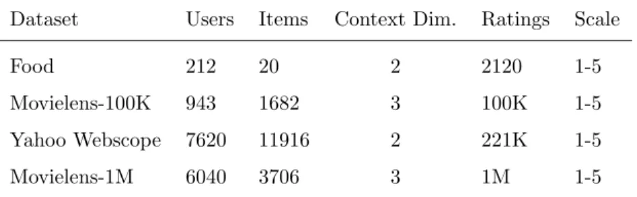
Datasets. We conduct experiments on three real datasets and one semi-synthetic dataset below, with Table 1 summarizing the basic information.
• Food dataset: This is a popular small-scale dataset obtained from the coauthor (H. Asoh) of [44]. It studies how much one subject wants to order a dish. It contains 6,360 ratings given by 212 users for 20 food menus. The data includes ratings in real situations and virtual situations (really hungry or just imagine). Following the advice of the data provider (H. Asoh), we only take ratings in real situations to study. Two popular context variables are selected: situation (hungry, normal, full) and menu
Table 1: Experiment dataset summary.
Dataset Users Items Context Dim. Ratings Scale
Food 212 20 2 2120 1-5
Movielens-100K 943 1682 3 100K 1-5
Yahoo Webscope 7620 11916 2 221K 1-5
Movielens-1M 6040 3706 3 1M 1-5
genre (Japanese, Chinese, Western), which are user and item contexts respectively.
• Movielens-100K1: This is a popular dataset collected by the GroupLens Research Project at the University of Minnesota. It consists of 100K ratings in a {1, 2, 3, 4, 5} scale from around 943 users on 1,682 movies. Each user rated at least 20 movies. We pick three types of user contextual information that are most interesting to us: the gender, occupation, and age. There are 20 occupations such as lawyer, doctor, and artist, and the ages are divided into 5 groups: ≤18, 18-25, 25-35, 35-50 and≥50. • Movielens-1M1: This is a larger version of Movielens-100K. It contains
1,000,209 anonymous ratings of approximately 3,900 movies made by 6,040 users. Other information is the same as that of Movielens-100K, such as rating scale and occupation category. The timestamp is separated to hour and day contextual information.
• Yahoo Webscope Movies2: This dataset is provided as part of the Yahoo! Research Alliance Webscope program. It contains 221K ratings in a {1, 2, 3, 4, 5} scale for about 11,916 movies evaluated by 7,620 users, as well as various user contexts such as gender and age, and item contexts including the timestamp. In order to explore the extent that
1http://movielens.org/ 2http://research.yahoo.com/
contexts affect user ratings, we follow the data preprocessing steps in [25] to generate six semi-synthetic datasets from the original data using two user-context features “age” and “gender” in the raw Yahoo dataset by the following steps.
1. We convert the age feature into a three-class categorical variable according to three groups: above 50, between 18 and 50 and below 18.
2. We generate a random featurex∈ {0, 1} for each rating to replace the original gender feature to artificially affect the ratings.
3. We randomly picka×100% movies from the dataset.
4. We randomly chooseb×100% ratings from these movies to increase (decrease) the rating value by one if the corresponding x = 1 (x
= 0) unless the rating value is already 5 (1). E.g., if 50% of the dataset’s movies are randomly picked and 10% of the selected movies’ rating would be modified, the synthetic dataset with a = 0.9 and
b = 0.5 has 90% of its items altered with profiles that have half of their ratings changed. Six semi-synthetic datasets are generated with
a= 0.1,0.5,0.9 andb= 0.1,0.5,0.9. In this way, a largea×b has a greater contextual influence on the ratings.
Evaluation metrics. We use two popular metrics in evaluation, the Root Mean Square Error (RMSE) and Mean Absolute Error (MAE):
RM SE= s P y∈Ωtest(y−yˆ) 2 |Ωtest| (35) M AE = P y∈Ωtest|y−yˆ| |Ωtest| (36) whereydenotes the true rating, ˆyis the estimated rating, and Ωtest represents
the test set. The smaller the RMSE and MAE, the better the recommendation performance. 5×5-fold cross-validation results are reported.
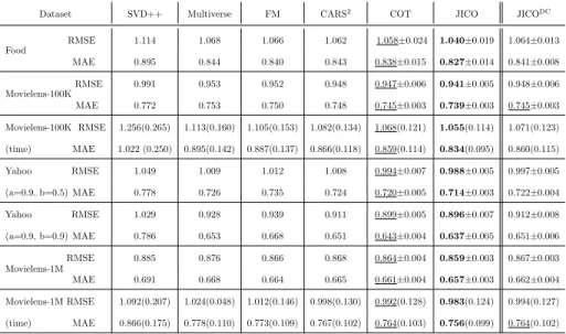
Table 2: Recommendation performance comparison on four datasets, with seven scenarios in total. In each scenario, the best results (achieved by JICO) are in bold and the second best (achieved by COT) ones are underlined. We report the standard deviation of 5×5 cross
validation results for COT and JICO except the time split results. For the time split results (time), we indicate the performance degradation of each method in a pair of parentheses.
Dataset SVD++ Multiverse FM CARS2 COT JICO JICODC
Food RMSE 1.114 1.068 1.066 1.062 1.058±0.024 1.040±0.019 1.064±0.013 MAE 0.895 0.844 0.840 0.843 0.838±0.015 0.827±0.014 0.841±0.008 Movielens-100KRMSE 0.991 0.953 0.952 0.948 0.947±0.006 0.941±0.005 0.948±0.006 MAE 0.772 0.753 0.750 0.748 0.745±0.003 0.739±0.003 0.745±0.003 Movielens-100K (time) RMSE 1.256(0.265) 1.113(0.160) 1.105(0.153) 1.082(0.134) 1.068(0.121) 1.055(0.114) 1.071(0.123) MAE 1.022 (0.250) 0.895(0.142) 0.887(0.137) 0.866(0.118) 0.859(0.114) 0.834(0.095) 0.860(0.115) Yahoo (a=0.9, b=0.5) RMSE 1.049 1.009 1.012 1.008 0.994±0.007 0.988±0.005 0.997±0.005 MAE 0.778 0.726 0.735 0.724 0.720±0.005 0.714±0.003 0.722±0.004 Yahoo (a=0.9, b=0.9) RMSE 1.029 0.928 0.939 0.911 0.899±0.005 0.896±0.007 0.912±0.008 MAE 0.786 0.653 0.668 0.651 0.643±0.004 0.637±0.005 0.651±0.006 Movielens-1M RMSE 0.885 0.876 0.866 0.868 0.864±0.004 0.859±0.003 0.867±0.003 MAE 0.691 0.668 0.664 0.665 0.661±0.004 0.657±0.003 0.662±0.004 Movielens-1M (time) RMSE 1.092(0.207) 1.024(0.048) 1.012(0.146) 0.998(0.130) 0.992(0.128) 0.983(0.124) 0.994(0.127) MAE 0.866(0.175) 0.778(0.110) 0.773(0.109) 0.767(0.102) 0.764(0.103) 0.756(0.099) 0.764(0.102)
4.2. Recommendation Performance Comparison
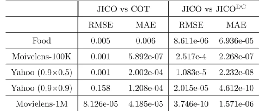
Table 2 compares the performance of each model on the four datasets. The best and second-best results in each case, achieved by JICO and COT, are highlighted in bold and underline, respectively. Table 3 reports thepvalues of
t-tests performed for the results of JICO and COT, and JICO and JICODC, to
confirm the statistical significance. We have the following observations: • The context-aware models all significantly outperform the context-free
model SVD++, suggesting that rich contextual information is beneficial to improve recommendation performance. JICO improves over SVD++ by 6.6%, 5.0%, 5.8%, 12.9%, 2.9% in RMSE and 7.6%, 4.2%, 8.2%, 19.0%, 4.9% in MAE on the Food, Movielens-100K, Yahoo (0.9 × 0.5), Yahoo (0.9×0.9) and Movielens-1M datasets respectively. There is a clear gap between the improvements of different datasets, since the effect of contex-tual information is not always the same in different situations. The more
Table 3:p-value for the results of JICO and COT, and JICO and JICODCreported in Table
2.
JICO vs COT JICO vs JICODC
RMSE MAE RMSE MAE
Food 0.005 0.006 8.611e-06 6.936e-05 Moivelens-100K 0.001 5.892e-07 2.517e-4 2.268e-07 Yahoo (0.9×0.5) 0.001 2.002e-04 1.083e-5 2.232e-08 Yahoo (0.9×0.9) 0.158 1.208e-04 2.015e-05 4.612e-10 Movielens-1M 8.126e-05 4.185e-05 3.746e-10 1.571e-06
relevant the contexts and entities, the greater the improvement in general. • Among context-aware methods, Multiverse and FM have similar perfor-mance on all datasets, while inferior to CARS2, COT, and JICO. E.g.,
JICO improves over the best of Multiverse and FM by 2.4%, 1.1%, 2.0%, 3.4%, 0.81% in RMSE and by 1.5%, 1.5%, 1.7%, 2.5%, 1.1% in MAE on Food, Movielens-100K, Yahoo (0.9×0.5) and Yahoo (0.9 ×0.9) and Movielens-1M datasets. The limited performance of Multiverse and FM is likely limited due to treating contexts as a dimension similar to users and items. However, contexts play different roles as users and items in a recommendation. Therefore, modelling contexts as semantic operators, as in CARS2, COT, and JICO, can further improve the performance of
context-aware recommendation.
• JICO achieves the best performance consistently in all cases studied. Al-though CARS2, COT, and JICO all model contexts as semantic operators,
the interaction between contexts and user/item is separately modelled in CARS2 and COT, leading to double-counting.
Hence, JICO combines joint interaction in MF and context operation in CARS2and COT to achieve superior performance over all other methods.
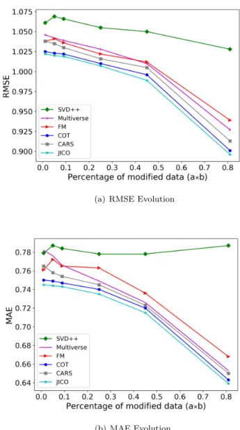
(a) RMSE Evolution
(b) MAE Evolution
Figure 3: Recommendation performance variation with respect to the amount of contextual influence on Yahoo semi-synthetic dataset.
4.3. Varying Contextual Influence
The six semi-synthetic Yahoo datasets enable us to study the various degrees of contextual influence, as controlled by a×b, as in [25]. Figure 3 depicts the recommendation performances with respect to the growth of contextual influence. We can see the following:
• Over all degrees of contextual influence, JICO consistently gives the best performance, with COT the second, and CARS2the third. JICO improves
over FM, Multiverse, CARS2, and COT by 4.3%, 2.3%, 1.7%, 1.3% and
0.9% on high context dataset with a×b = 0.81. It means that JICO can make better use of context in a high context influence situation. This again demonstrates the benefits of combining joint interaction in MF and context operation in COT and CARS2.
• The performance gain of context-aware methods over the context-free method, SVD++, continues increasing with the greater degree of con-textual influence. This indicates that greater concon-textual influence can lead to greater performance improvement. All the context-aware methods are benefiting from such influence growth.
• Relative to context-aware methods, the influence of contexts on SVD++ is quite limited. It is interesting to note that on the left side of the MAE subfigure, SVD++ slightly outperformed Multiverse, indicating that when the contextual information is weak, Multiverse may not model it properly, leading to a negative impact.
4.4. Realistic Evaluation on Time Split
Although we report the cross-validation results popularly done in perfor-mance evaluation, it is actually not a realistic assessment in practice. This is because rating data come in sequence and we can only use past data to predict future data, not vice versa. Considering this situation, we present experiments about time split that is a realistic case embodying two challenges: one iscold
start, and the other isimbalanced training/testing data. We carry out this re-alistic study by splitting the training/test data at a time point, rather than random splitting in cross-validation.
For this time split study, we use Movielens-100K and Movielens-1M and split each dataset into training (80%) and test (20%) data by its attribute “timestamp”. The results are reported in the rows labelled as “Movielens-100K (time)”and 1M (time)” in Table 2. Compared to the “Movielens-100K”and “Movielens-1M” rows, we can see that all results get worse (larger errors) with time split. In Table 2, we indicate the increased amount of error in a pair of parentheses in the “Movielens-100K (time)” and “Movielens-1M (time)” rows. SVD++ suffers the most degradation (e.g., 0.265/0.250 in RMSE/MAE on Movielens-100K, and 0.207/0.175 in RMSE/MAE on Movielens-1M). JICO has the least degradation (only 0.114/0.095 in RMSE/MAE on Movielens-100K, and 0.124/0.099 in RMSE/MAE on Movielens-1M).
Due to the time constraint, although the amount of training data are the same for time split and cross-validation (random split), there are actually less entity (user/item) information available for the time split case. For example, new users and movies after the time split point have no information available for training in the time split case while the cross-validation case could have such information due to random sampling. In other words, the effective contextual information is less in the time split case than in the cross-validation case. The least degradation achieved by JICO again shows the superiority of our two-layer approach.
4.5. Context Analysis and Interpretation
As a context-aware model, JICO enables interpretation of context impor-tance, which is captured by the context weight vector wk. Figure 4(a)
de-picts different context weight percentage on Movielens-100K and Food datasets. The greater the percentage, the higher the importance. This figure shows that context variable “Situation” has more influence on rating than context “Menu genre” on the Food dataset. On Movielens-100K, the most important context
is occupation (50%), followed by age (41%), and genders impact is relatively small (<10%). This allows an intuitive understanding of the effects of different contexts on ratings.
As a latent factor model, JICO also learns latent representations of contexts to reveal the relationships among them. Since the context latent vector’s di-mension can vary, we follow Wuet al. [45] to use Principal Component Analysis (PCA) to reduce the context vector’s dimension to 2 to visualize the relation-ships among different context values in a 2-D space. In the context importance analysis above, we found that “Occupation” is a dominate context on Movielens-100K dataset so we visualize this context in 2-D space via PCA in Fig. 4(b). The figure mainly reflects two facts. We can observe:
• The location of each occupation reflects the occupation’s rating bias. The top right tends to give higher ratings while the lower left tends to give lower ratings. For instance, the average ratings for the engineer, programmer, educator, and artist are 3.541, 3.568, 3.670, and 3.441, respectively. We can see that the “artist” tends to give lower ratings, due to their unique artistic taste. In contrast, the “educator” occupation tends to give a higher rating to movies than “artist”, which is expected.
• The distance between different points reflects their preference similarities and potential relationships. E.g., programmer and engineer are close, indicating they have a similar preference on movies, while doctor and educator are far apart, showing that they tend to have different tastes. The context latent vector representations in JICO, with PCA, can help reveal relationships among context values. Such analysis can help us gain important insights and use such information in subsequent applications.
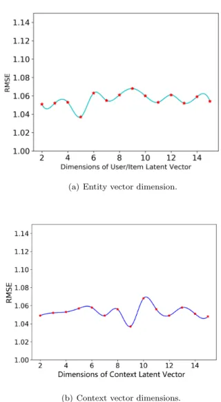
4.6. Impact of Latent Vector Dimensions
Finally, we show the sensitivity of JICO (in RMSE) to the latent vector dimensions of user/item and contexts on the Food dataset in Figs. 5(a) and 5(b), respectively. The user/item or context dimension is fixed to 4 when testing
(a)
(b)
Figure 4: Contextual information analysis: (a) Different context weight percentages on the Movielens-100K and Food datasets. (b) Occupation representations in 2-D space, with di-mension reduced by PCA.
the other. We can see that the best dimensionality of user/item vectordeis 5
(a) Entity vector dimension.
(b) Context vector dimensions.
Figure 5: Recommendation performance sensitivity with respect to JICO latent vector dimen-sions on the Food dataset.
variations, which are much smaller than those observed in similar curves in COT [27]. This indicates that JICO is much less sensitive to the latent vector dimension settings than COT.
5. Conclusion
This paper proposed JICO, a novel context-aware recommendation model combining joint interaction with the context operation. It models the relation-ships between user/item and contexts more properly by addressing limitations of previous models while leveraging their virtues. We performed experiments on four datasets to show the superior recommendation performance and var-ious interesting studies, such as varying contextual influence and time split recommendation. The results show that JICO consistently outperforms other state-of-the-art models in all cases studied.
In future, we can further develop JICO in two directions. Firstly, since JICO can be treated as a generic supervised learning model, we can potentially add deep models with multiple layers to further improve the model performance [46, 47]. Secondly, Lawrence and Urtasun [48] proposed a non-linear matrix factorization for collaborative filtering, which can be extended to tensor factor-ization. This can further extend JICO and other recommendation models based on the tensor operation to capture non-linear interactions in data.
Acknowledgment
The authors would like to thank the anonymous reviewers for their insightful comments, which have helped to improve the quality of this paper.
References
[1] D. Jannach, M. Zanker, A. Felfernig, G. Friedrich, Recommender systems: an introduction, Cambridge University Press, 2010.
[2] G. Linden, B. Smith, J. York, Amazon. com recommendations: Item-to-item collaborative filtering, IEEE Internet Computing 7 (1) (2003) 76–80. [3] J. L. Herlocker, J. A. Konstan, L. G. Terveen, J. T. Riedl, Evaluating collaborative filtering recommender systems, ACM Transactions on Infor-mation Systems (TOIS) 22 (1) (2004) 5–53.
[4] B. Sarwar, G. Karypis, J. Konstan, J. Riedl, Item-based collaborative filter-ing recommendation algorithms, in: Proceedfilter-ings of the 10th International Conference on World Wide Web, ACM, 2001, pp. 285–295.
[5] M. D. Ekstrand, J. T. Riedl, J. A. Konstan, et al., Collaborative filtering recommender systems, Foundations and TrendsR in Human–Computer
In-teraction 4 (2) (2011) 81–173.
[6] X. Su, T. M. Khoshgoftaar, A survey of collaborative filtering techniques, Advances in artificial intelligence 2009.
[7] J. Bobadilla, F. Ortega, A. Hernando, A. Guti´errez, Recommender systems survey, Knowledge-based systems 46 (2013) 109–132.
[8] Y. Koren, R. Bell, C. Volinsky, Matrix factorization techniques for recom-mender systems, Computer 42 (8).
[9] L. Baltrunas, B. Ludwig, F. Ricci, Matrix factorization techniques for con-text aware recommendation, in: Proceedings of the fifth ACM conference on Recommender systems, ACM, 2011, pp. 301–304.
[10] A. Mnih, R. R. Salakhutdinov, Probabilistic matrix factorization, in: Ad-vances in neural information processing systems, 2008, pp. 1257–1264. [11] X. Ma, P. Sun, G. Qin, Nonnegative matrix factorization algorithms for
link prediction in temporal networks using graph communicability, Pattern Recognition 71 (2017) 361–374.
[12] Y. Koren, Collaborative filtering with temporal dynamics, Communications of the ACM 53 (4) (2010) 89–97.
[13] J. Fan, T. W. Chow, Non-linear matrix completion, Pattern Recognition 77 (2018) 378–394.
[14] J. Fan, T. W. Chow, Matrix completion by least-square, low-rank, and sparse self-representations, Pattern Recognition 71 (2017) 290–305.
[15] F. O. de Fran¸ca, G. P. Coelho, F. J. Von Zuben, Predicting missing values with biclustering: A coherence-based approach, Pattern Recognition 46 (5) (2013) 1255–1266.
[16] J. Sublime, B. Matei, G. Cabanes, N. Grozavu, Y. Bennani, A. Cornu´ejols, Entropy based probabilistic collaborative clustering, Pattern Recognition 72 (2017) 144–157.
[17] G. Adomavicius, A. Tuzhilin, Context-aware recommender systems, in: Recommender systems handbook, Springer, 2011, pp. 217–253.
[18] C. Palmisano, A. Tuzhilin, M. Gorgoglione, Using context to improve pre-dictive modeling of customers in personalization applications, IEEE trans-actions on knowledge and data engineering 20 (11) (2008) 1535–1549. [19] G. Adomavicius, R. Sankaranarayanan, S. Sen, A. Tuzhilin, Incorporating
contextual information in recommender systems using a multidimensional approach, ACM Transactions on Information Systems (TOIS) 23 (1) (2005) 103–145.
[20] L. Baltrunas, F. Ricci, Context-based splitting of item ratings in collabo-rative filtering, in: Proceedings of the third ACM conference on Recom-mender systems, ACM, 2009, pp. 245–248.
[21] U. Panniello, A. Tuzhilin, M. Gorgoglione, C. Palmisano, A. Pedone, Ex-perimental comparison of pre-vs. post-filtering approaches in context-aware recommender systems, in: Proceedings of the third ACM conference on Recommender systems, ACM, 2009, pp. 265–268.
[22] Y. Li, J. Nie, Y. Zhang, B. Wang, B. Yan, F. Weng, Contextual recom-mendation based on text mining, in: Proceedings of the 23rd International Conference on Computational Linguistics: Posters, Association for Com-putational Linguistics, 2010, pp. 692–700.
[23] E. Zhong, W. Fan, Q. Yang, Contextual collaborative filtering via hierar-chical matrix factorization, in: Proceedings of the 2012 SIAM International Conference on Data Mining, SIAM, 2012, pp. 744–755.
[24] X. Liu, K. Aberer, Soco: a social network aided context-aware recom-mender system, in: Proceedings of the 22nd international conference on World Wide Web, ACM, 2013, pp. 781–802.
[25] A. Karatzoglou, X. Amatriain, L. Baltrunas, N. Oliver, Multiverse recom-mendation: n-dimensional tensor factorization for context-aware collabo-rative filtering, in: Proceedings of the fourth ACM conference on Recom-mender systems, ACM, 2010, pp. 79–86.
[26] S. Rendle, Z. Gantner, C. Freudenthaler, L. Schmidt-Thieme, Fast context-aware recommendations with factorization machines, in: Proceedings of the 34th international ACM SIGIR conference on Research and development in Information Retrieval, ACM, 2011, pp. 635–644.
[27] S. Wang, C. Li, K. Zhao, H. Chen, Context-aware recommendations with random partition factorization machines, Data Science and Engineering 2 (2) (2017) 125–135.
[28] L. De Lathauwer, B. De Moor, J. Vandewalle, A multilinear singular value decomposition, SIAM journal on Matrix Analysis and Applications 21 (4) (2000) 1253–1278.
[29] L. R. Tucker, Some mathematical notes on three-mode factor analysis, Psychometrika 31 (3) (1966) 279–311.
[30] H. Lu, K. N. Plataniotis, A. N. Venetsanopoulos, A survey of multilinear subspace learning for tensor data, Pattern Recognition 44 (7) (2011) 1540– 1551.
[31] S. Rendle, Factorization machines, in: Data Mining (ICDM), 2010 IEEE 10th International Conference on, IEEE, 2010, pp. 995–1000.
[32] A. Coates, A. Y. Ng, The importance of encoding versus training with sparse coding and vector quantization, in: Proceedings of the 28th Inter-national Conference on Machine Learning (ICML-11), 2011, pp. 921–928. [33] T. V. Nguyen, A. Karatzoglou, L. Baltrunas, Gaussian process
factoriza-tion machines for context-aware recommendafactoriza-tions, in: Proceedings of the 37th international ACM SIGIR conference on Research & development in information retrieval, ACM, 2014, pp. 63–72.
[34] S. Wang, C. Li, K. Zhao, H. Chen, Learning to context-aware recommend with hierarchical factorization machines, Information Sciences 409 (2017) 121–138.
[35] Y. Shi, A. Karatzoglou, L. Baltrunas, M. Larson, A. Hanjalic, Cars2: Learning context-aware representations for context-aware recommenda-tions, in: Proceedings of the 23rd ACM International Conference on Con-ference on Information and Knowledge Management, ACM, 2014, pp. 291– 300.
[36] Q. Liu, S. Wu, L. Wang, Cot: Contextual operating tensor for context-aware recommender systems., in: AAAI, 2015, pp. 203–209.
[37] T. Mikolov, I. Sutskever, K. Chen, G. S. Corrado, J. Dean, Distributed rep-resentations of words and phrases and their compositionality, in: Advances in neural information processing systems, 2013, pp. 3111–3119.
[38] M. Baroni, R. Zamparelli, Nouns are vectors, adjectives are matrices: Rep-resenting adjective-noun constructions in semantic space, in: Proceedings of the 2010 Conference on Empirical Methods in Natural Language Pro-cessing, Association for Computational Linguistics, 2010, pp. 1183–1193. [39] R. Socher, B. Huval, C. D. Manning, A. Y. Ng, Semantic
composition-ality through recursive matrix-vector spaces, in: Proceedings of the 2012 joint conference on empirical methods in natural language processing and
computational natural language learning, Association for Computational Linguistics, 2012, pp. 1201–1211.
[40] R. Socher, A. Perelygin, J. Wu, J. Chuang, C. D. Manning, A. Ng, C. Potts, Recursive deep models for semantic compositionality over a sentiment tree-bank, in: Proceedings of the 2013 conference on empirical methods in nat-ural language processing, 2013, pp. 1631–1642.
[41] T. G. Kolda, B. W. Bader, Tensor decompositions and applications, SIAM review 51 (3) (2009) 455–500.
[42] H. Lu, K. N. Plataniotis, A. N. Venetsanopoulos, Multilinear Subspace Learning: Dimensionality Reduction of Multidimensional Data, CRC Press, 2013.
[43] Y. Koren, Factorization meets the neighborhood: a multifaceted collabo-rative filtering model, in: Proceedings of the 14th ACM SIGKDD inter-national conference on Knowledge discovery and data mining, ACM, 2008, pp. 426–434.
[44] C. Ono, Y. Takishima, Y. Motomura, H. Asoh, Context-aware preference model based on a study of difference between real and supposed situation data, User Modeling, Adaptation, and Personalization (2009) 102–113. [45] S. Wu, Q. Liu, L. Wang, T. Tan, Contextual operation for recommender
systems, IEEE Transactions on Knowledge and Data Engineering 28 (8) (2016) 2000–2012.
[46] G. E. Hinton, S. Osindero, Y.-W. Teh, A fast learning algorithm for deep belief nets, Neural computation 18 (7) (2006) 1527–1554.
[47] Q. Liu, S. Wu, L. Wang, Collaborative prediction for multi-entity inter-action with hierarchical representation, in: Proceedings of the 24th ACM International on Conference on Information and Knowledge Management, ACM, 2015, pp. 613–622.
[48] N. D. Lawrence, R. Urtasun, Non-linear matrix factorization with gaussian processes, in: Proceedings of the 26th Annual International Conference on Machine Learning, ACM, 2009, pp. 601–608.