(will be inserted by the editor)
Multiple Imputation Ensembles (MIE) for dealing
with missing data
Aliya Aleryani * · Wenjia Wang ·
Beatriz de la Iglesia
the date of receipt and acceptance should be inserted later
Abstract Missing data is a significant issue in many real-world datasets yet there are no robust methods for dealing with it appropriately. In this paper we propose a robust approach to dealing with missing data in classification problems: Multiple Imputation Ensembles (MIE). Our method integrates two approaches: multiple imputation and ensemble methods and compares two types of ensembles: bagging and stacking.
We also propose a robust experimental setup using 20 benchmark datasets from the UCI Machine Learning repository. For each dataset, we introduce increasing amounts of data Missing Completely At Random (MCAR). Firstly, we use a number of Single/Multiple imputation methods to recover the missing values and then ensemble a number of different classifiers built on the imputed data.
We assess the quality of the imputation by using dissimilarity measures. We also evaluate the MIE performance by comparing classification accuracy on the complete and imputed data. Furthermore, we use the accuracy of simple imputation as a benchmark for comparison. We find that our proposed ap-proach combining multiple imputation with ensemble techniques outperform others, particularly as missing data increases.
Keywords Missing data· Multiple imputation · Dissimilarity measures·
Classification algorithms·Ensemble techniques * Corresponding author
A. Aleryani
University of East Anglia Norwich NR4 7TJ E-mail: [email protected]
W. Wang
University of East Anglia Norwich NR4 7TJ E-mail: [email protected]
B. De La Iglesia
University of East Anglia Norwich NR4 7TJ E-mail: [email protected]
1 Introduction
Many real-world datasets have missing or incomplete data [22, 23, 75]. Since the accuracy of most machine learning algorithms for classification, regression, and clustering could be affected by the completeness of datasets, processing and dealing with missing data is a significant step in data mining and machine learning processes. Yet this is still under-explored in the literature [61, 11, 70, 69, 28, 49, 68].
A Few strategies have been commonly used to handle incomplete data [48, 30, 34]. For regression problems specifically where missing data has been more widely studied [48, 38, 39, 36, 55], Multiple Imputation (MI) has shown advantage over other methods [48, 72] because the multiple imputed values give a mechanism to capture the uncertainty reflected in missing data. However, work is still needed to address the problem of missing data in the context of data mining algorithms. Particularly, it is timely to experiment with the concept of multiple imputation and how to apply to classification problems.
The aim of this work is therefore to conduct a thorough investigation on how to effectively apply MI for classification algorithms. We propose an en-semble that combines multiple models produced by MI, and we investigate the ways for combining different ensemble mechanisms with MI methods to achieve best results.
Our proposed method, MIE, is evaluated and compared with other alter-natives under some simulated scenarios of increasing uncertainty in terms of missing data. For this, we create an experimental environment using datasets selected from the university of California Irvine (UCI) Machine learning repos-itory [47]. For each dataset, we use a mechanism called Missing Completely At Random (MCAR) to generate missing data through removing the values of chosen attributes and instances with a variable probability. Therefore, we pro-duce several experimental datasets which contain increasing amount of data MCAR.
In those scenarios, we investigate how increasing the amount of missing data affects the performance of competing approaches for handling missing data. They include the algorithm’s internal mechanism for handling missing data, single imputation, machine learning imputation and our proposed MIE.
1.1 The problem of missing data
Little and Rubin [48] have defined the missing data problem based on how missing data is produced in the first place and they proposed three main categories as follows: Missing Completely at Random (MCAR), Missing at Random (MAR), and Missing not at Random (MNAR). The categorisation is important because it affects the biases that may be inherent in the data, and therefore the safety of approaches such as imputation. Missing Completely at Random (MCAR) occurs when an instance missing for a particular variable is independent of any other variable and independent of the missing data. It can
be said that for MCAR missing data is not related to any other factor known or unknown in the study. This represents the safer environment for imputation to operate. Missing at Random (MAR) happens when the probability of having missing value in a record may depend on the known values of other attributes but not on the missing data. There are some inherent biases in data MAR, but it may be still safe to analyse this type of data without explicitly accounting for the missing data. Missing not at Random (MNAR) occurs when the probability of the instance having a missing value depends on unobserved values. This is also termed anon-ignorableprocess and is the most difficult scenario to deal with. In this paper we focus on addressing MCAR data, the safest environment in which imputation could operate and one that is often encountered. Further work will investigate the other mechanisms.
Horton et al. [39] have further categorised the patterns of missing data into monotone and non-monotone. Monotone patterns of missing data imply that the same data points have missing values in one or more features, so specific points are affected by missing data. They state that the patterns are concerned with which values are missing, whereas, the mechanisms are concerned with why data is missing.
We focus in this study on non-monotone MCAR data so our missing data affects multiple data points with no particular relation between data missing for different attributes for the same data points.
1.2 Mechanisms for dealing with missing data
In practice, there are four popular approaches that have been used to deal with incomplete data: complete analysis [48], statistical imputation methods [4, 24, 34, 59], machine learning algorithms for imputation [51, 40, 59, 57, 52] and algorithms with a built-in mechanism to deal with missing data [51, 74, 43, 10, 25]. The first three approaches rely on pre-processing of the data to either remove or replace missing values. The last approach comprises of a mechanism in the algorithms themselves to produce models taking account of the missing data. We provided a detailed explanation of the different approaches in our previous work [2].
We also studied how different classification algorithms such as C4.5 [51, 52], Na¨ıve Bayes (NB) [10, 45], Support Vector Machines (SVMs) [74, 16, 5], and Random Forest (RF) [21, 7] and their implementations in Weka, our platform of choice, can treat missing values [2]. A number of classification algorithms (e.g. C4.5 [52] and RF [43]) have been constructed with a mechanism called
fractional method to cope with missing data. Na¨ıve Bayes ignores features with missing values thus only the complete features are used for classification [10, 45]. SVMs do not deal with missing values [46] but its implementation in Weka, SMO, performs simple imputation [32]. In this work we investigate PART, in addition to the previous classifiers, which is also capable of treating missing data when constructing a partial tree as C4.5 does [25].
The rest of this paper is organised as follows: Section 2 reviews related research; the methods used in our paper are described in Section 3 followed by our experimental set-up in Section 4; Section 5 details out the results of this study; this is followed by a discussion and conclusions in Section 6.
2 Related work
MI has been studied in the context of statistical analysis [58, 57, 55]. After that, it has been widely applied in many studies such as in survival analysis [41, 73], epidemiological and clinical trials [65, 44], medical studies [72, 56], and longitudinal studies [63, 50]. The application of MI with ensemble learning for classification has rarely been used in the literature. We review a few published papers that have discussed the problem of missing data in the context of classification algorithms and the use of MI methods.
Silva-Ram´ırez et al. [62] proposed a method for simple imputation based on a Multi-Layer Perceptron (IMLP) and a method for multiple data imputation that combines a Multi-Layer Perceptron andk-Nearest Neighbour (k-NN al-gorithm to impute missing data (MIMLP). The problem under consideration was monotone MCAR missing data. The methods were compared with the traditional imputation methods such as mean, Hot-deck, and regression-based imputation. Their results showed that the MIMLP method performed best for numeric variables and the IMLP method performed better with categori-cal variables. Imputation by MLP methods offered some advantages for some datasets though statistical test for significance were not performed.
Liu et al. [49] proposed a credal classification method with adaptive im-putation for incomplete pattern. In credal classification objects can belong to multiple classes and meta-classes. The method has two stages. First a record is classified based on the available information if the class is non ambiguous. However, when the record is hard to classify then it goes to the second step which involves imputation and later classification. In the imputation phase, Self-Organized Map (SOM) is used to in combination with k-NN to obtain good accuracy while reducing computational burden.
A correlation-based low-rank matrix completion (LRMC) method was de-veloped by Chen et al. [12]. The method applies LRMC to estimate missing data then uses a weighted Pearson’s correlation followed by K-Nearest Neigh-bour (k-NN) search to choose the most similar samples. Furthermore, they proposed an ensemble learning to integrate multiple imputed values for a spe-cific sample to improve imputation performance. The proposed method was tested on both traffic flow volume data and benchmark datasets. Further in-vestigation was conducted to test the performance of the imputation in the classification tasks. Their proposed correlation-based LRMC and its ensem-ble learning method achieved better performance than traffic flow imputation methods such as temporal nearest average imputation (TNAI), temporal av-erage imputation (TAI), probabilistic principal component analysis (PPCA), low-rank matrix completion (LRMC).
Tran et al. [69] proposed a method that introduces multiple imputation with an ensemble and compared the proposed method with others that use simple imputation. Ten datasets were collected from UCI repository. The en-semble achieved better classification accuracy than the other methods. How-ever, they only applied C4.5 as a classification algorithm and used one method to perform multiple imputation on relatively small datasets.
Garciarena and Santana [31] studied the relationship between different im-putation methods and missing data patterns using ten datasets from the UCI repository and a set of fourteen different classifiers such as decision trees, neural networks, support vector machines, k-NN and logistic regression. The result shows that the performance of individual classifiers is statistically differ-ent when using various imputation methods. They concluded that the key to selecting proper imputation methods is to check first the patterns of missing data.
Tran et al. [70] further proposed methods incorporating imputation (sin-gle/multiple) with feature selections and clustering to improve classification accuracy and also the computational efficiency of imputation.
A new hybrid technique based on a fuzzy c-Means clustering algorithm, mutual information feature selection and regression models (GFCM) was de-veloped by Sefidian and Daneshpour [61]. The aim was to find a set of similar records with high dependencies for a missing record and then apply regression imputation techniques within the group to estimate missing values for that record. The method showed statistical significant differences in most cases in comparison with mean imputation, kNNI, MLPI [62], FCMI [53], and IARI [64].
3 MIE for classification
MI is a promising method that has been used to replace missing values by randomly drawing several imputed values from the distribution of unknown data [48, 55]. Unlike in simple imputation, the uncertainty is reflected as the imputation process will result in various plausible values. There are a number of methods to impute data that we will explore in our work, and explain below. We also explore different methods to ensemble the results obtained from the different imputed values, as the ensemble represents a method for combining the evidence from the different models to arrive a final classification which should encompass the degree of missing data.
3.1 Imputation methods
3.1.1 Multivariate Imputation by Chained Equations (MICE)
Fully Conditional Specification (FCS) is a method of MI that was firstly de-veloped by Kennickell [42]. It defines a conditional density function to specify
an imputation model for each missing predictor (variable) one by one, then it-erates the imputation over that model. Multivariate Imputation with Chained Equations (MICE), an algorithm developed by Buuren [8], is based on FCS but the imputation can be also applied for data that has no multivariate distribution. For each variable with missing values, the algorithm starts by identifying an imputation model for each column with missing values. After that, the imputation will be performed based on random draws from the ob-served data. The process is repeated based on the number of iterations set-up and the number of variables with missing values.
3.1.2 Expectation-Maximisation with Bootstrapping (EMB)
Honaker et al. [38] have developed an EMB algorithm for handling missing data that combines the EM algorithm with a bootstrapping approach. The EM algorithm is an iterative approach developed by Dempster et al. [17]. Starting with the Expectation and then the Maximisation step, the algorithm aims to estimate the model parameters by iteratively performing the following. Firstly, in the Expectation step (E-step), the likelihood function is evaluated by considering the current estimate of the model parameters. Second, in the Maximisation step (M-step), the parameters are updated to maximize the likelihood function. Next, the E-step updates the parameters fromM-step to determine the new distribution.
On the other hand, bootstrapping is a mechanism used to estimate a sample distribution from original data with or without replacement. EMB works by repeatedly drawing a bootstrap with replacement from the original data M
times, for theM required imputations; then, EM is run which firstly assumes a particular distribution, then initialise a mean and variance values for the missing data in each bootstrap generated. Then the likelihood function is estimated by considering the current estimate of the model parameters (mean and covariance). Then the parameters are updated to maximise the likelihood model. The expectation and the maximisation steps are repeated until the values converge [37].
3.2 Ensemble methods
An ensemble is a technique for combining models used in machine learning. It was introduced by Tukey [71] when he built an ensemble of two different regression models. Since then it has been then broadly studied and reviewed in classification tasks [20, 19, 6, 76]. The idea of an ensemble is to induce a set of base learners (classifiers), then their predictions are aggregated in some way to obtain a better classification. This can have advantages over relying on a single model as a combined model may be more precise and accurate. Furthermore, Breiman [6] explained the usefulness of ensembles with unstable classifiers that are easily affected by changes to the training data such as decision trees and neural networks.
An ensemble can be categorised according to the underlying machine learn-ing algorithms used into two main types: homogeneous and heterogeneous. A
homogeneous ensemble is constructed from learners of the same type, e.g. a set of decision trees. On the other hand, when the strategy is to combine different types of learners such as decision trees, neural networks or Bayesian networks then we have aheterogeneous ensemble.
In general application, the aim of constructing an ensemble is to achieve a classification accuracy that is higher than any of the individual learner. Thus, the individual learners are expected to be accurate with an error rate better than random guess, and diverse so two classifiers make different errors when predicting a new instance. A number of methods for constructing a diverse ensemble have been developed [19, 27, 6, 13]. Below is an explanation of the most popular ensemble methods which are bagging and stacking.
3.2.1 Bagging:
Bagging, (also known as Bootstrap Aggregation), is one of common ensemble methods that can be applied to classification and regression problems [19, 52]. It is used to reduce the variance between models by generating additional training sets from the original data [52]. One such method is where a propor-tion of data points are randomly chosen with replacement by using bootstrap
mechanism which generates multiple training sets; each has approximately 63% of the training data points [66, 52]. Then a same base learner (e.g. deci-sion trees) is run in parallel on these training sets. As a result, an ensemble of different models will be generated. To make the prediction for a new data, the final decision is made by a majority vote of the individual predictions obtained from the different models [19, 52].
3.2.2 Stacking:
In the context of ensemble learning, meta-learning is the process of learning from the multiple learners and their outputs on the original training data. Such method is efficient when individual classifiers mis-classify the same patterns [54]. The method was introduced by Wolpert [76] and refers to a construction mechanism that uses the output of classifiers instead of the training data to build the ensemble. A stacking ensemble can be implemented in two or more layers. In the first layer, a number of base learners are trained on the entire training set then produce (level-0) models. Then the predictions of the individual models are used as input attributes (meta-level attributes) to the ensemble. The target of the original training set is appended to the (meta-level attributes) to form a new set of predictions, ((meta-level-1) model. This set is used to train a meta classifier in the ensemble. The meta classifier can be trained based on the predicated class label or the probabilities generated from (level-0) models [67]. This model is used to estimate the final prediction in the ensemble.
3.3 Framework for MIE
Our ensemble for MI works as follows. We first generate a series of increasing missing data under MCAR assumption. We then impute the artificial train-ing datasets and generate five imputed datasets ustrain-ing two different MI tech-niques: MICE and EMB as described in section 3.1. We next use these datasets to train classifiers and build our Bagging and Stacking ensembles. For our
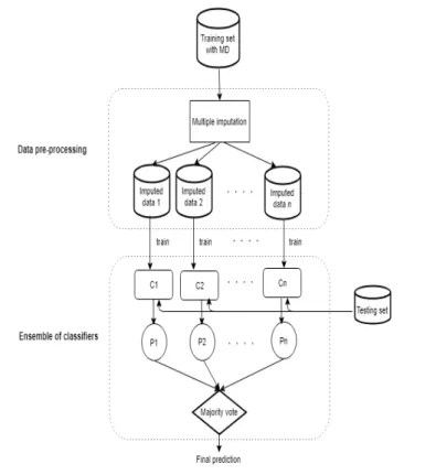
Bagging ensemble we train homogeneous classifiers (same classifiers) on the imputed datasets. We then combine the predictions of the models obtained from a separate test data using a majority vote method. This method aggre-gates the predictions from the individual models and chooses the class that has been predicted most frequently as the final prediction, as illustrated in Fig. 1. Therefore, the Bagging ensemble is evaluated using a hold-out test set. This can be viewed as an alternative method for bagging in which multiple imputed datasets may be more dissimilar to each other hence generate more diverse models. On the other hand, Fig. 2 represents the construction of our
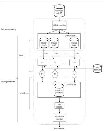
Stackingensemble showing two layers. The first one involves the multiple im-puted datasets trained by a number of learners (heterogeneous classifiers) to generate different models. The models are tested then against a separate test set to make a new dataset of predictions. This new dataset is combined with the actual class of the test set to construct the (level-1) dataset which is used as an input for the second layer. In this layer we train a meta classifier and then we evaluate the performance of the ensemble using 10-fold cross-validation.
4 Experimental set-up
4.1 Datasets
For our study, a collection of 20 benchmark datasets were obtained from the UCI machine learning repository [47]. The datasets have different sizes and feature types (numerical real, numerical integer, categorical and mixed) as shown in Table 1. They were all complete datasets, that is they have no missing values, except Post-operative Patient dataset where three records with missing values have been deleted.
4.1.1 Data Preparation
Before conducting experiment we solved the problem of the sparse datasets we have, LSVT and Forest Cover Type. LSVT has five attributes with zero values so we deleted those features. On the other hand, we transform Forest Cover Type by taking the attributes that represent Wilderness Area (4 binary columns) and Soil Type (40 binary columns) then reducing each to a single column with multiple values. So the first new column has a numerical value of (1 to 4) which represents the presence of a particular area while the second indicates the soil type with a value (1 to 40). Additionally, we followed Clark et
Fig. 1 The bagging ensemble framework takes imputed datasets as inputs to train different classifiersC1, ...,Cnin layer 1. The predictions made by individual classifiers,P1, ...,Pn, are
combined by the majority vote method.
al. [15] mechanism of treating Abalone as a 3-category classification by group-ing classes 1-8, 9 and 10, and 11 on so that we can improve the classification process.
Some datasets are provided with separate train and testing sets. The rest have been partitioned usingStratifiedRemoveFolds filter in weka to retain the class distributions with a ratio of 70% training and 30% testing, except Forest Cover Type, our largest dataset, where 60% of data is used for training and 40% for testing.
Table 2 shows the mean accuracy and the standard deviation of the classi-fiers (J48, NB, PART, SMO and RF) obtained on the testing sets by training on the original data with no missing values. Those classification results for the complete data are used then as the benchmarks to study how missing data affects the accuracy and performance of the algorithms when various meth-ods for dealing with missing data are used. Note that we run RF five times with different random seeds as it obtains different results in each run given its stochastic nature. The RF classifier performs better than other classifiers in nine of the datasets. Then SMO is the second best classifier, working best on
Fig. 2 The stacking ensemble framework takes imputed datasets as inputs to train classifiers
C1, ...,Cn. The predictions made by individual classifiers,P1, ...,Pn, are used to form a new
data to be used to train a meta classifier in the second layer.
five datasets out of twenty, while J48 and PART work best on three datasets each. The performance of NB is the worst compared to the other classifiers.
Then we test the performance of multiple classifiers on multiple datasets using Friedman test to check which classifiers outperform others. The test shows a significant difference (p-value<0.05) in performance so we proceed with post hoc test, Nemenyi test. The Critical Difference diagram as a result of applying Nemenyi test is shown in Fig. 3. The figure illustrates that RF behave significantly better than PART and NB although there is no statistical differences within each group, i.e. no statistical significant between RF, SMO and J48. Similarly, the performance difference for J48, PART, NB and SMO is not statistically significant.
4.2 Missing Data Generation
To create scenarios for testing with increasing missing data, some values in the training sets are removed completely at random as follows: Firstly, 10% (then 20%, 50%) of the attributes are randomly selected to remove data with
Table 1 The details of the datasets collected for the experiments. The # symbol next to the dataset denotes that it has come with a separate test set.
No. Dataset #Features #Instances #Classes Feature Types 1 PostOperativePatient 8 87 2 Integer, Categorical
2 Ecoli 8 336 8 Real
3 Abalone 8 4177 3 Integer, Real and Categorical
4 TicTacToe 9 958 2 Categorical
5 BreastTissue 10 106 6 Real
6 Statlog 20 1,000 2 Integer, Categorical
7 Spect # 22 276 2 Categorical
8 Flags 30 194 8 Integer, Categorical
9 BreastCancer 31 569 2 Real
10 Chess 36 3,196 2 Categorical
11 Connect-4 42 67,557 2 Categorical
12 ForestCoverType 54 581,012 7 Integer, Categorical
13 ConnectionistBench 60 208 2 Real
14 HillValley # 101 606 2 Real
15 UrbanLandCover # 148 168 9 Integer, Real 16 EpilepticSeizure 179 11,500 5 Integer, Real
17 Semeion 265 1,593 2 Integer
18 LSVT 309 126 2 Real
19 HAR # 561 10,299 6 Real
20 Isolet # 617 7,797 26 Real
Table 2 The mean accuracy of the classifiers and standard deviation for the complete datasets obtained based on test set. A best accuracy values for each dataset are in bold.
Dataset J48 NB PART SMO RF Avg
PostOperativePatient 71.43 64.29 71.43 60.71 64.29(0.00) 66.43(0.00) Ecoli 82.14 83.04 82.13 83.04 80.89(1.20) 82.25(0.24) Abalone 63.43 58.91 62.21 65.23 65.36(0.71) 63.028(0.14) TicTacToe 84.33 72.73 88.09 98.75 95.17(1.14) 87.81(0.23) BreastTissue 65.71 57.14 62.86 57.14 64.57(1.56) 61.48(0.31) Statlog 72.37 76.28 69.97 76.27 74.95(1.22) 73.97(0.24) Spect 66.84 64.71 65.24 67.91 69.95(1.48) 66.93(0.30) Flags 57.81 48.44 53.13 35.94 60.00(2.61) 51.06(0.52) BreastCancer 95.24 93.65 92.06 97.88 95.98(0.80) 94.96(0.16) Chess 99.25 88.08 98.97 95.40 99.06(0.16) 96.15(0.03) Connect-4 79.31 72.11 78.39 76.06 81.94(0.07) 77.56(0.01) ForestCoverType 93.71 62.16 91.4 71.70 96.58(0.02) 83.11(0.01) ConnectionistBench 72.46 69.57 65.22 81.15 84.35(1.89) 74.55(0.38) HillValley 48.15 51.44 48.15 53.08 56.71(1.80) 51.51(0.36) UrbanLandCover 67.65 77.91 69.83 74.56 81.30(0.53) 74.25(0.11) EpilepticSeizure 48.53 43.33 49.62 27.52 68.17(0.40) 47.43(0.08) Semeion 92.84 91.34 98.49 97.74 95.40(0.10) 95.16(0.02) LSVT 66.67 51.19 97.62 76.19 85.71(1.69) 75.48(0.34) HAR 93.85 75.85 94.47 98.31 97.95(0.20) 92.09(0.04) Isolet 83.45 82.36 82.81 95.83 93.97(0.31) 87.68(0.06)
Fig. 3 Critical Difference diagram showing statistically significant differences between clas-sifiers. The bold line connecting classifiers means that they are not statistically different.
the following chosen rates 5%, 15%, 30% and 50% of the records, respec-tively. We repeat the process of selection and removing five times so different
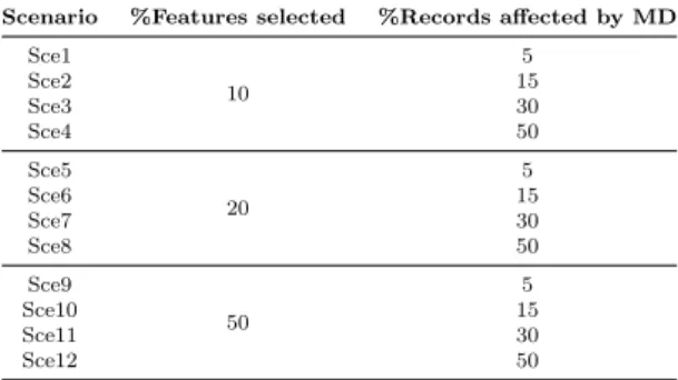
features/records may be affected by missing data each time. As a result, 12 artificial datasets are produced from each of the original datasets each time and those have multiple levels of missing data. In total, we generate (20*12*5= 1260) datasets. Table 3 summarises the experimental scenarios artificially cre-ated.
Table 3 Experimental scenarios with missing data artificially created. Scenario %Features selected %Records affected by MD
Sce1 10 5 Sce2 15 Sce3 30 Sce4 50 Sce5 20 5 Sce6 15 Sce7 30 Sce8 50 Sce9 50 5 Sce10 15 Sce11 30 Sce12 50
In our experiments, the models are tested on separated test data. How-ever, for the stacking ensemble, the results reported represent 10-fold cross-validation as the predictions of the separated test sets are used to construct a new dataset for the second layer of the stack ensemble.
4.3 Comparative methods
4.3.1 Building models with missing data (MD)
In Section 1.2 we discussed that the chosen algorithms have their own way of dealing with missing data internally. We therefore pass all the data includ-ing missinclud-ing data to the algorithms without pre-processinclud-ing. Such models are referred to as J48 MD, NB MD, PART MD, SMO MD and RF MD.
4.3.2 Simple imputation (SI)
To test simple imputation, the numerical attributes are replaced with their mean and the categorical attributes with their mode. Then the produced datasets after imputation are used for classification model building. In our results the models with single imputation are referred to as J48 SI, NB SI, PART SI, SMO SI and RF SI.
4.3.3 Random forest imputation (RFI)
We use a RF imputation package (missForest) implemented in R to replace missing values using a RF algorithm. The algorithm starts with filling
incom-plete data by median if they are numeric or mode if they are categorical. Then it updates missing values by using proximity from random forest and iterates the imputation a number of times. Finally, the imputed value for an attribute with missing values is the weighted average of non missing values if it is nu-meric or the mode if it is nominal. We set up the number of iterations to perform the imputation to 5 and the number of trees that grow in each forest to 300. In our results the models that used RFI are referred to as J48 RFI, NB RFI, PART RFI, SMO RFI and RF RFI.
4.4 Proposed MIE methods
The following steps have been undertaken to test the bagging and stacking en-semble. First, MICE and Amelia packages inR, which implement Multivariate Imputation with Chained Equation and Expectation Maximisation with Boot-strap algorithms, respectively, are applied to generate five imputed datasets. For MICE, we set the predictive mean match as the imputation method, the number of iterations to perform the imputation to 20 and the number of the imputed datasets to 5. For Amelia, we used 5 as the number of imputations, too. Additionally, we perform the imputation in parallel when processing large and high dimensional datasets.
The multiple imputed datasets are used as inputs to train the classifiers and for our bagging ensemble, we aggregate the predictions obtained by the models by the majority vote method. One base learner is used as the classifier. Our classifiers of choice for the bagging ensemble are J48 [51], NB [45], PART [26], SMO [60] and RF [43] (as implemented inWeka) with their default options for classifying the data. On our results, such models are referred to as MICE Hom and EMB Hom, depending on the method to perform the imputation in the first place.
A second ensemble approach tested is to build a stacking ensemble, where the training datasets are used to perform the imputation then to train all chosen classifiers to generate several models. These models are used as inputs to the first layer of the stack. The predictions of the different models on the testing set are used to form a new dataset for level-1 in the ensemble. Then we train a meta classifier in this new dataset in the second layer. For testing the stacking ensemble, we perform 10-fold cross validation to evaluate the perfor-mance of models. These are referred to as MICE SE and EMB SE depending on the MI method.
4.5 Evaluating classification methods
We use the classification accuracy as the metric for our comparisons of perfor-mance. We compare between all the approaches looking for differences in the algorithms’ performance on each scenario separately. We perform Wilcoxon
Signed Rank test with Finner’s procedure for correcting the p-values for pair-wise comparison testing with a significance level of α= 0.05 [18, 29] with a number of controls separately as follows:
We perform two different statistical tests when evaluating the performance of classifiers over the datasets as follows:
1. When comparing multiple classifiers over multiple datasets, we use the method described by Demˇsar [18], including the Friedman test and the post hoc Nemenyi test which is represented as a Critical Difference (CD) diagram, with a significance level ofα= 0.05.
2. The Wilcoxon Signed Rank test is applied for performing pairwise com-parison. We use a control algorithm, the performance of the classifier on SI, with a significance level atα= 0.05.
4.6 Evaluating imputation methods
Numerous statistical methods are used to check the variation between and within the multiple imputed datasets [3, 8, 35, 1]. These involve graphical rep-resentations such as Histogram, density and quantile-quantile plots [1]. Others suggest the use of numerical comparisons such as means and standard devia-tions [35]. In this study instead we propose the use of dissimilarity, as used in the context of clustering algorithms [14, 9, 33], to evaluate the quality of the imputation methods.Dissimilarity is a numeric measurement of the degree of difference between data points. We check the quality of the imputation by com-paring each imputed data point with its original counterpart. In that way we can measure the dissimilarity between each pair of points (original/imputed). We can then aggregate dissimilarity across the whole dataset to arrive to a measure of quality of the imputation, with imputations that produce points closer to the original being considered better than those where the dissimilarity is greater.
As we have different data types in our datasets, i.e. numeric, categorical, mixed, we use the weighted overall dissimilarity formula proposed by Gower [33], the Gower Coefficient, to compute the distance dis(a,b) between each data point,a, in the original dataset and the corresponding data point, b, in the artificial dataset after performing MI as follows:
dis(a, b) = PN f=1w (f) ab dis (f) ab PN f=1w (f) ab (1)
whereNdenotes the total number of features in a dataset,wis the assigned weight to a feature (we setw=1 for each feature) andf is a feature which can be either numerical or categorical.
Before we apply the formula to measure distance, we standardise each nu-merical attribute,f, into a comparable range using the standardised measure,
z−score, to avoid attributes with a larger range having a bigger effect on the
distance measurement. For this we use the following equation:
x0 =z(xf) = (xf−mf)/sf (2)
wherexdenotes a value in an attribute,mthe mean of attribute andsis the mean absolute deviation for that attribute. Then we compute the distance, dis(f)ab, as follows:
dis(f)ab =|x0af −x0bf| (3) The contribution of each categorical attribute to the overall dissimilarity dis(f)ab = 0 ifxaf andxbf are identical otherwisedis
(f) ab = 1 .
The overall aggregated dissimilarity function remains in the same range [0,1]. Finally, we average the distance of all records to obtain the mean distance between the original and imputed data.
5 Results
In order to understand how different algorithms behave under different im-putation regimes, we began by investigating each algorithm separately. In particular, we applied our proposed methods that combine MI with ensem-ble techniques, MIE, along with the comparative approaches as described in Section 4.3. We therefore study the performance of the internal mech-anism of the algorithms for handling missing data (e.g for J48, J48 MD, NB MD, PART MD, SMO MD and RF MD), the simple imputation (J48 SI, NB SI, PART SI, SMO SI and RF SI), the RF imputation (J48 RFI, NB RFI, PART RFI, SMO RFI and RF RFI). Our proposed MIE methods are repre-sented by the combination between MI methods with bagging (MICE Hom, EMB Hom) and stacking ensembles (MICE SE, and EMB SE). The details of the results can be found from the authors.
5.1 Classification performance
For each of the classifier/imputation methods studied, we applied the Friedman statistical test [18] to compare the performance of the imputation methods including our proposed approach. The test compares the mean ranks of the classifiers on a number of datasets as follows: with 7 algorithms (i.e. variations on imputation regimes) and 20 datasets,z it is distributed according to the zdistribution with 7 - 1 = 6 and (7 - 1)*(20 - 1) = 114 degrees of freedom.
If we use a significance level ofα= 0.05, the critical value of zis 2.18.
For the J48 algorithm, Table 4 summarises the mean rank for the different imputation/ensemble methods on each of the artificial datasets in each scenario separately. Hint: lowest rank means better performance. On average, for J48 the stacking ensemble with EMB (EMB SE) obtained a better rank hence
better overall classification accuracy, with MICE SE second best. J48 SI was the worst.
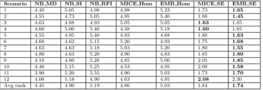
Similar results were obtained for the NB, PART and SMO algorithms as illustrated in Tables 5, 6, and 7. In each case the EMB SE algorithm produced the best performance in terms of ranking and hence overall accuracy on differ-ent datasets. For both NB and PART, MICE SE was second best. However, for SMO in Table 7, RFI was a close match to MICE SE. For RF, shown in Table 8 EMB Hom was the best in most scenarios whereas the internal mechanism of RF for handling MD showed worse performance than others in most cases.
Table 4 The mean rank for J48 on different imputation methods along with proposed approach on all dataset affected by missing data in all scenarios. The value in bold indicates that the algorithm performs better than others.
Scenario J48 MD J48 SI J48 RFI MICE Hom EMB Hom MICE SE EMB SE
1 5.08 5.38 4.13 4.88 3.60 2.50 2.45 2 5.35 5.30 4.25 4.50 3.78 2.60 2.23 3 5.58 5.58 4.10 4.18 3.93 2.10 2.55 4 4.93 5.53 4.68 4.50 3.70 2.33 2.35 5 5.38 5.60 3.98 4.53 3.68 2.45 2.40 6 5.25 5.68 4.43 4.10 3.55 2.48 2.53 7 5.35 5.20 5.05 4.15 3.48 2.40 2.38 8 5.20 5.53 4.58 4.80 3.05 2.48 2.38 9 4.93 5.33 4.80 4.75 3.60 2.48 2.13 10 5.30 5.13 4.70 4.50 3.43 2.23 2.73 11 5.00 5.33 4.58 4.50 2.90 2.63 3.08 12 4.88 5.65 4.15 4.20 3.13 3.30 2.70 Avg rank 5.19 5.44 4.45 4.47 3.49 2.50 2.49
Table 5 The mean rank of NB in combination with different imputation methods and of our proposed approach on all dataset affected by missing data for different scenarios. The value in bold indicates that the algorithm performs better than others.
Scenario NB MD NB SI NB RFI MICE Hom EMB Hom MICE SE EMB SE
1 4.40 5.05 4.98 4.98 5.23 1.73 1.65 2 4.55 4.73 5.05 4.95 5.40 1.88 1.45 3 4.63 4.88 4.93 5.05 5.05 1.63 1.85 4 4.60 5.00 5.40 4.38 5.18 1.60 1.85 5 4.55 4.95 5.40 4.93 4.68 1.88 1.63 6 4.68 4.63 5.15 5.20 4.93 1.75 1.68 7 4.63 4.63 5.18 5.03 5.20 1.80 1.55 8 4.80 4.63 5.20 4.90 4.83 1.85 1.80 9 4.18 4.80 5.28 4.85 5.00 2.05 1.85 10 4.48 5.15 5.25 4.53 4.95 2.08 1.58 11 3.90 5.20 5.55 4.90 5.03 1.73 1.70 12 4.08 5.18 4.90 4.63 4.85 2.08 2.30 Avg rank 4.45 4.90 5.19 4.86 5.03 1.84 1.74
So far we have used the Friedman test to compute the average ranks. The test also gives us the ability to compute a p-value, to discern if the al-gorithm performs significantly different to others according to the average rank obtained. Table 4 presents the p-values resulting from application of the Friedman test for each scenario and each algorithm, and shows that the per-formance of the different imputation methods when combined with a given classifier were significantly different. The symbol∗ denotes that the test was significant p < 0.05. J48, NB, and PART were statistically different when
Table 6 The mean rank of PART in combination with different imputation methods and of our proposed approach on all dataset affected by missing data for different scenarios. The value in bold indicates that the algorithm performs better than others.
Scenario PART MD PART SI PART RFI MICE Hom EMB Hom MICE SE EMB SE
1 4.48 5.45 4.78 4.63 3.65 2.45 2.58 2 4.43 5.58 4.78 4.58 3.35 2.93 2.38 3 4.80 5.43 4.78 4.35 3.33 2.88 2.45 4 4.85 5.55 4.85 4.28 3.65 2.40 2.43 5 4.30 5.43 4.75 5.40 3.10 2.58 2.45 6 4.73 5.48 4.55 4.73 3.28 2.70 2.55 7 4.75 5.13 4.70 4.90 3.03 3.13 2.38 8 4.35 5.93 5.03 4.23 2.93 2.95 2.60 9 4.98 5.53 5.15 4.58 3.10 2.73 1.95 10 4.63 5.50 5.00 5.00 3.03 2.50 2.35 11 5.28 5.70 4.85 4.25 2.60 2.75 2.58 12 4.38 5.75 4.88 4.30 3.18 2.93 2.60 Avg rank 4.66 5.54 4.84 4.60 3.18 2.74 2.44
Table 7 The mean rank of SMO in combination with different imputation methods and of our proposed approach on all dataset affected by missing data for different scenarios. The value in bold indicates that the algorithm performs better than others.
Scenario SMO MD SMO SI SMO RFI MICE Hom EMB Hom MICE SE EMB SE
1 4.68 5.00 3.95 4.30 3.75 3.53 2.80 2 4.83 5.10 4.05 3.78 4.00 3.30 2.95 3 4.60 5.15 3.63 4.63 3.83 3.40 2.78 4 4.80 5.15 3.48 4.43 3.60 3.18 3.38 5 4.20 4.85 3.90 3.80 4.30 3.25 3.70 6 4.80 5.05 4.05 3.75 4.08 3.00 3.28 7 4.93 5.65 3.65 4.05 3.78 3.13 2.83 8 4.90 5.08 3.48 4.00 3.75 3.53 3.28 9 4.85 5.03 3.93 3.90 4.03 3.45 2.83 10 4.85 4.98 4.00 3.75 4.10 3.08 3.25 11 4.38 4.93 2.95 4.58 4.03 3.80 3.35 12 5.03 5.25 2.93 3.93 3.83 3.48 3.58 Avg rank 4.74 5.10 3.66 4.07 3.92 3.34 3.16
Table 8 The mean rank of RF in combination with different imputation methods and of our proposed approach on all dataset affected by missing data for different scenarios. The value in bold indicates that an algorithm performs better than others.
Scenario RF MD RF SI RF RFI MICE Hom EMB Hom MICE SE EMB SE
1 5.10 4.65 3.58 3.90 3.20 4.00 3.58 2 4.95 4.78 3.85 4.10 2.93 4.12 3.23 3 4.88 4.35 3.60 4.5 3.03 3.63 4.03 4 4.65 4.80 3.75 4.55 2.85 4.00 3.40 5 4.63 4.40 3.43 3.28 4.70 3.88 3.70 6 5.38 4.45 3.58 4.08 3.05 3.45 4.03 7 5.10 4.33 3.68 4.05 3.00 4.15 3.70 8 4.55 4.23 3.45 4.23 2.88 4.33 4.35 9 5.63 4.90 3.70 3.63 3.03 4.03 3.10 10 5.08 4.48 4.03 3.45 3.25 3.93 3.80 11 4.88 4.60 3.08 3.83 2.90 4.15 4.58 12 5.25 4.20 2.85 3.93 3.03 4.30 4.45 Avg rank 5.00 4.51 3.55 3.96 3.15 4.00 3.83
different imputation methods were applied in all scenarios tested. The perfor-mance of SMO was significant in most cases while RF was the same in half of the cases.
We also used the Wilcoxon signed rank for pairwise comparison with a con-trol algorithm. This test computes the median (not average) accuracy among all datasets. We chose the performance of the classifiers applied to data im-puted by SI as a control as this is a form of naive imputation which may be frequently used and is often used as a control against new data imputation
Table 9 The p-values resulting from the Friedman test for comparing the performance of each classifier with different imputation methods separately. The symbol (*) shows that the performance of the classifiers are statistically different when applying different imputa-tion/ensemble methods.
Scenario Classifiers
J48 NB PART SMO RF
1 6.33E-07* 7.03E-13* 5.34E-06* 0.03* 0.07 2 3.76E-07* 5.50E-13* 5.88E-06* 0.02* 0.03* 3 1.34E-08* 9.59E-12* 1.21E-05* 0.01* 0.11 4 1.71E-07* 3.00E-12* 5.79E-07* 0.01* 0.04* 5 7.05E-08* 4.37E-12* 8.65E-08* 0.34 0.19 6 3.59E-07* 4.00E-12* 6.29E-06* 0.02* 0.02* 7 8.73E-08* 1.59E-12* 1.33E-05* 0.00* 0.09 8 2.46E-08* 1.24E-10* 5.22E-07* 0.04* 0.15 9 6.39E-08* 6.13E-10* 3.54E-09* 0.02* 0.00* 10 1.06E-06* 3.58E-11* 3.76E-08* 0.03* 0.13 11 1.74E-05* 4.04E-13* 1.82E-08* 0.05 0.02* 12 8.55E-05* 1.37E-07* 6.46E-06* 0.01* 0.01*
methods. MI combined with an ensemble in the case of the J48 algorithm (i.e. EMB Hom, MICE SE and EMB SE) was statically significant better than the control in all cases as shown in Table 10. On the other hand, MICE HOM mod-els and J48 RFI were significantly different in a few scenarios. The internal mechanism of J48 for handling MD was not different than SI.
For the NB algorithm, results are shown in Table 11. We can see that only the combination between MI and stacking (MICE SE and EMB SE) per-formed statistically differently from the control while other methods showed no difference.
For PART, as shown in Table 12, the combination between MI with en-sembles (EMB Hom, MICE SE and EMB SE) were better than the control in all cases. On the other hand MICE Hom, PART RFI and the internal method were significantly different to the control in a few scenarios.
For SMO, performance for the EMB SE approach is better in most but not all cases and similarly for MICE SE, as illustrated in Table 13. SMO RFI was better than the control only when the ratio of missingness increases. The EMB Hom method was significantly better than the control when low missing values were encountered.
For RF, Table 14 presents the comparison with the control and shows some improvements when EMB Hom was used. For all other approaches to missing data there appears to be little difference.
5.2 Quality of the imputed data
Here we first evaluate the quality of imputation methods used, i.e. how far is the imputed data from the real data. We used the normalized euclidean distance as explained in Section 4.6 to compute the mean dissimilarity between the imputed and the original data. We divide our analysis by the feature type (i.e. numerical, categorical or mixed) as imputation may work differently for
Table 10 The median accuracy for J48 on different imputation/ensemble methods along with proposed approach resulting from Wilcoxon signed rank test. The symbol (*) indicates that the algorithm performs better than the control.
Scenario J48 MD J48 SI J48 RFI MICE Hom EMB Hom MICE SE EMB SE 1 75.32 75.30 75.43 75.57 76.07* 81.05* 81.31* 2 75.24 75.24 75.69* 75.69* 76.11* 80.65* 81.34* 3 74.90 74.95 75.40* 75.40* 75.98* 81.01* 80.67* 4 75.03 74.86 75.08* 75.20* 75.86* 80.34* 80.21* 5 75.19 75.13 75.64* 75.78* 76.39* 80.86* 80.85* 6 75.39 75.11 75.60* 75.64* 76.28* 80.61* 80.44* 7 75.00 75.10 75.37 75.54 76.25* 80.15* 80.65* 8 74.54 73.93 74.54* 74.27 76.38* 79.71* 79.44* 9 75.63 75.21 75.31 75.34 76.70* 81.08* 81.09* 10 74.82 75.36 75.14 75.33 76.92* 80.74* 80.28* 11 74.31 73.84 74.91* 74.41 76.63* 78.78* 78.33* 12 73.04 71.92 73.50* 73.74* 75.63* 77.06* 77.66*
Table 11 The median accuracy for NB on different imputation/ensemble methods along with proposed approach resulting from Wilcoxon signed rank test. The symbol (*) indicates that the algorithm performs better than the control.
Scenario NB MD NB SI NB RFI MICE Hom EMB Hom MICE SE EMB SE 1 69.91 69.94 69.77 69.91 69.76 81.80* 81.84* 2 69.99 70.0 69.80 69.92 69.83 81.83* 82.12* 3 70.09 70.07 69.78 69.88 69.93 81.42* 81.58* 4 69.74 69.92 69.54 69.67 69.78 81.15* 81.32* 5 69.89 70.04 69.56 69.96 69.92 81.16* 81.62* 6 69.90 70.06 69.50 69.77 69.90 81.47* 81.53* 7 70.07 70.14 69.62 69.85 69.91 81.22* 81.47* 8 69.66 69.94 69.35 69.53 69.74 80.41* 80.11* 9 70.13 70.31 69.37 70.15 70.013 81.04* 81.36* 10 70.03 69.91 69.18 70.31 69.79 81.35* 81.33* 11 70.25 69.73 69.07 69.83 69.62 79.86* 79.44* 12 70.25 69.07 69.09 69.54 69.49 78.11* 78.20*
Table 12 The median accuracy for PART on different imputation/ensemble methods along with proposed approach resulting from Wilcoxon signed rank test. The symbol (*) indicates that the algorithm performs better than the control.
Scenario PART MD PART SI PART RFI MICE Hom EMB Hom MICE SE EMB SE
1 75.89 75.51 75.56 75.46 77.11* 80.92* 81.03* 2 75.68* 75.14 75.60* 75.35 77.18* 79.81* 80.80* 3 75.62 74.99 75.34 75.61 77.34* 79.75* 80.08* 4 75.29 74.93 74.84 75.44 76.64* 79.86* 80.54* 5 75.98* 75.40 75.64 75.41 77.53* 80.27* 80.70* 6 75.55 75.09 75.65 75.34 77.26* 80.15* 80.54* 7 75.20 75.21 75.36 74.66 77.68* 79.42* 80.38* 8 75.19* 73.40 74.24* 74.74* 77.23* 78.32* 79.15* 9 75.58 75.23 75.11 75.35 77.65* 80.33* 81.02* 10 75.28* 74.80 74.92 74.69 77.55* 79.81* 80.22* 11 74.21* 73.15 74.20* 75.00* 77.75* 77.98* 78.40* 12 73.85* 71.70 72.85* 72.57 75.82* 76.45* 77.57*
different data types. The number of datasets in each group are 10, 5 and 5, respectively.
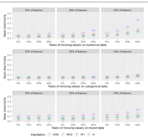
The three plots at the top of Fig. 4 represents the mean dissimilarity be-tween the real and the imputed values using EMB, MICE, RFI and SI with respect to the numerical datasets. In most of the scenarios RFI produced im-puted data closer to the real data as the mean dissimilarity was very close to 0. EMB was a close match to RFI followed by MICE. However, imputed data by SI was the worst as it was further from the real data specially with increasing uncertainty. With respect to the categorical data, the plots in the middle of the figure shows that the mean dissimilarity for all imputation methods devised
Table 13 The median accuracy for SMO on different imputation/ensemble methods along with proposed approach resulting from Wilcoxon signed rank test. The symbol (*) indicates that the algorithm performs better than the control.
Scenario SMO MD SMO SI SMO RFI MICE Hom EMB Hom MICE SE EMB SE 1 76.12 75.61 75.93 76.52 76.36 81.37* 81.61* 2 75.75 75.62 75.74 76.27 76.12 81.55* 81.75* 3 75.66 75.54 76.27* 76.24 76.32* 81.11* 81.22* 4 75.46 75.40 76.38* 75.50 76.33* 80.95* 80.82* 5 76.23 75.99 75.61 76.35 76.26 80.93 81.25 6 75.71 75.79 76.01 76.14 75.85 81.12* 81.10* 7 75.28 75.04 75.84* 76.01 76.08* 80.94* 81.13* 8 74.99 75.00 75.51 75.94 75.44 79.75 79.95* 9 76.14 76.00 75.94 76.46 76.44 81.16* 81.50* 10 75.21 75.16 75.17 76.41 75.42 81.17* 80.93* 11 74.89 74.61 75.43 74.93 74.28 79.23 79.16* 12 73.27 73.26 75.20* 73.19 73.67 77.81* 78.23
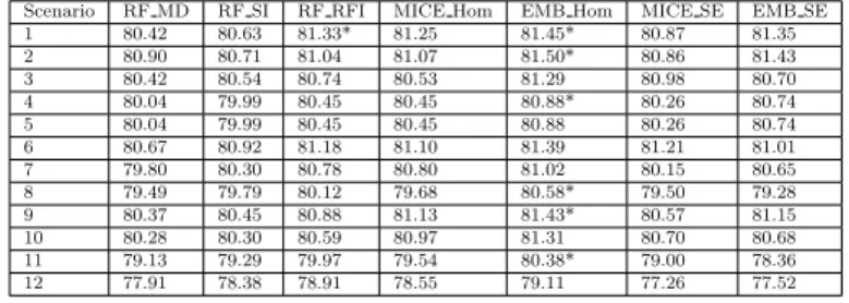
Table 14 The median accuracy for RF on different imputation/ensemble methods along with proposed approach resulting from Wilcoxon signed rank test. The symbol (*) indicates that the algorithm performs better than the control.
Scenario RF MD RF SI RF RFI MICE Hom EMB Hom MICE SE EMB SE 1 80.42 80.63 81.33* 81.25 81.45* 80.87 81.35 2 80.90 80.71 81.04 81.07 81.50* 80.86 81.43 3 80.42 80.54 80.74 80.53 81.29 80.98 80.70 4 80.04 79.99 80.45 80.45 80.88* 80.26 80.74 5 80.04 79.99 80.45 80.45 80.88 80.26 80.74 6 80.67 80.92 81.18 81.10 81.39 81.21 81.01 7 79.80 80.30 80.78 80.80 81.02 80.15 80.65 8 79.49 79.79 80.12 79.68 80.58* 79.50 79.28 9 80.37 80.45 80.88 81.13 81.43* 80.57 81.15 10 80.28 80.30 80.59 80.97 81.31 80.70 80.68 11 79.13 79.29 79.97 79.54 80.38* 79.00 78.36 12 77.91 78.38 78.91 78.55 79.11 77.26 77.52
were close to each other and to the real data though EMB produced the best performance for most scenarios. In the case of categorical data, all methods tested were efficient in terms of recovering missing values. On the other hand, different imputation methods behave differently with the mixed data type as shown at the bottom of the figure EMB produced data that was more similar to the real data as the mean dissimilarity did not exceed 0.1 in the worst case. RFI became second best followed by MICE. Again the SI was the worst in all cases.
5.3 Classification results by datatype
Finally, we analyse the efficiency of the imputation method based on different data types and we relate this to the performance of different classifiers. We do this separately for each classification algorithm. We present box plots showing the range of accuracies (max, min, median and any outliers) obtained for all the datasets of a given data type. The different scenarios in terms of % of missing data are represented in the x-axis, though we combined the results from the missing data affecting 10%, 20% and 50% features in one box plot as the same patterns were observed for each. The grey box plot in each graph represents the accuracy on the complete dataset, before any data is removed.
Fig. 4 The mean dissimilarity between the original and imputed data-points as a result of applying different imputation methods on numerical datasets where different percentage of features affected by missing data at different levels. The first row represents numerical data, the second represents categorical data and the last represents mixed data.
Fig. 5 shows the range of accuracies as box plots for the J48 algorithm applied on numerical (left), categorical (center), and mixed (right) datasets. On numerical datasets (the plot to the left), there are two clear methods that stand out as the median value for EMB SE and MICE SE was much higher than that of other methods and of the complete data for all levels of missing data. Also, the maximum accuracy of both EMB SE and MICE SE increased by about 10% compared with the complete data also for all levels of missing data. The EMB Hom method also shows some improved performance though not so marked. The other methods perform similarly to one another and to the complete data. For the categorical data (center plot), a similar pattern for median accuracy is observed with EMB SE and MICE SE showing best median performance, with some but not so marked improvement for maximum accuracy too. Overall median accuracy of most approaches decreased with increasing uncertainty but for EMB SE and MICE SE it was both higher than the complete data and that the other methods for most scenarios. On mixed datasets (right plot), the median accuracy of all approaches seemed to be similar to the complete data but the maximum average accuracy increased
when applying MICE SE and EMB SE. Outliers, represented by dots in the plot, were presented in all methods tested for mixed data.
Fig. 5 This figure contains box plots describing the overall average accuracy of J48 applied on imputed datasets using different imputation approaches along with the average accuracy on the complete data.
For the NB algorithm, similar results are shown in Fig. 6. However, for NB, MICE SE and EMB SE show performance improvements both in terms of maximum and medium average accuracies with respect to the mixed datasets. For PART, shown in Fig. 7 the median accuracy of PART MD, PART SI, PART RFI, MICE Hom and EMB Hom deteriorated for numerical datasets in comparison with the original data while the performance improves when MICE SE and EMB SE are applied. On categorical datasets, all different methods helped to keep performance similar to that of the complete data for low % of missing values but not when increasing the uncertainty. The performance of EMB Hom, MICE SE and EMB SE were the best on both categorical and mixed data.
For SMO, shown in Fig. 8 the median accuracy all methods on numerical datasets were similar to each other and to the complete data while the mini-mum accuracy of MICE SE and EMB SE increased by up to 10% compared with the completed data. Similarly, all approaches tested on the categorical data were relatively close. On mixed datasets, the median accuracy of the classifier seemed to be equal to the complete data but the maximum accuracy increased when applying MICE Hom, MICE SE and EMB SE.
Finally, the performance of RF with respect to different data types is shown in Fig. 9. All approaches tested where relatively similar so for this algorithm the method of imputation produced minor or no improvements. MICE SE and
Fig. 6 This figure contains box plots describing the overall average accuracy of NB applied on imputed datasets using different imputation approaches along with the average accuracy on the complete data.
Fig. 7 This figure contains box plots describing the overall average accuracy of PART applied on imputed datasets using different imputation approaches along with the average accuracy on the complete data.
EMB SE improved on maximum average accuracy for the categorical data but did not perform so well when increasing missing data was present. For the mixed data all approaches seemed similar.
Fig. 8 This figure contains box plots describing the overall average accuracy of SMO applied on imputed datasets using different imputation approaches along with the average accuracy for the complete data.
Fig. 9 This figure contains box plots describing the overall mean accuracy of RF applied on imputed datasets using different imputation approaches along with original data.
6 Discussion and conclusions
In this study, we investigate how different classification algorithms behave when using various methods for missing values imputation. We propose our
MIE approach to improve classification with missing data and compare it with other methods for dealing with missing data.
For J48, NB, PART and to a large extent for SMO, the proposed EMB SE produced the best performance for most levels of missing data with MICE SE being a closed second. For high levels of missing data SMO worked well with RFI. For the RF algorithm, however, EMB Hom produced the best perfor-mance in most cases. The differences in perforperfor-mance were statistically signif-icant in all cases for J48, NB, PART and in the majority of cases for SMO. For RF, they were statically significant in some scenarios only.
On the other hand, when comparing different approaches with a control method for imputation in the form of SI, we found that in most cases the pro-posed MIE techniques that rely on stacking (MICE SE and EMB SE) obtain statistically significantly better classification accuracy than the control when working with J48, NB, and PART. This was also true for SMO in the ma-jority of scenarios but not for RF where EMB Hom showed more significant improvements, consistently with our previous results.
It is not possible to directly compare our results to others working on related work due to different datasets and experimental setup. However, some comparisons are possible. For example, our findings, particularly for J48, are consistent with similar work done by Tran et al. [69] where they combined data imputed by MICE with an ensemble by using the majority vote method. Their proposed work achieved an improvement in terms of the classification accuracy. In our work we obtained further improvements on accuracy when using EMB imputation and stacking ensembles (MICE SE and EMB SE).
We proposed the use of dissimilarity to assess how far is the imputed data from the real data so that we can relate this to the performance of the algo-rithms. For numerical data RFI seems to perform best particularly for growing percentages of missing data. For categorical data EMB appears best by a very small margin, except for the highest missing data scenario. For mixed data EMB seems always best.
However, from further analysis of performance on each data type we can see that the imputation that recovers data best does not necessarily lead to a better classification performance. From the box plot analysis, we find that for all algorithms and data types except for RF, EMB SE and MICE SE pro-duce consistently better performance than the others, hinting at the fact that the ensemble plays a big part in producing good results. For RF again most methods seem to perform similarly though EMB SE and MICE SE are still consistently good performers. This indicates that the ensemble in itself pro-duces improvements irrespective of the quality of the imputation. As RF is already an ensemble algorithm, the advantages of MI for RF appear less ob-vious than for the others.
One of our important findings is that even in scenarios of increasing un-certainty, it is possible to obtain results similar or in some cases better than those obtained with the complete data, if the right imputation technique is used. This is an important finding as reasoning with missing data becomes then a lesser problem in the context of MCAR data. In this sense our proposed MIE
methods, particularly those using stacking as the ensemble method produce consistently good results. Although multiple imputation may consume time and memory particularly with large datasets, its advantages in terms of rep-resenting the uncertainty as well as the ability to introduce diversity for the ensemble classifiers enables us to improve classification accuracy for scenarios with large levels of missing data and for most classification algorithms tested. If an algorithm such as RF is used, then the imputation method appears less relevant, although a poor imputation method like SI can produce deteriorated performance particularly for mixed data.
As a future work, we can increase the number of imputed datasets to test if more diversity produces further improvements. We could also test the implications of MAR data, by providing a different experimental set up.
Acknowledgements
We acknowledge support from Grant Number ES/L011859/1, from The Busi-ness and Local Government Data Research Centre, funded by the Economic and Social Research Council to provide economic, scientific and social re-searchers and business analysts with secure data services.
Compliance with Ethical Standards
Conflict of InterestThe authors declare that they have no conflict of inter-est.
References
1. Abayomi, K., Gelman, A., Levy, M.: Diagnostics for multivariate imputa-tions. Journal of the Royal Statistical Society: Series C (Applied Statistics)
57(3), 273–291 (2008)
2. Aleryani, A., Wang, W., De La Iglesia, B.: Dealing with missing data and uncertainty in the context of data mining. In: International Conference on Hybrid Artificial Intelligence Systems, pp. 289–301. Springer (2018) 3. Azur, M.J., Stuart, E.A., Frangakis, C., Leaf, P.J.: Multiple imputation by
chained equations: what is it and how does it work? International journal of methods in psychiatric research20(1), 40–49 (2011)
4. Batista, G.E., Monard, M.C.: An analysis of four missing data treatment methods for supervised learning. Applied artificial intelligence 17(5-6), 519–533 (2003)
5. Boser, B.E., Guyon, I.M., Vapnik, V.N.: A training algorithm for opti-mal margin classifiers. In: Proceedings of the fifth annual workshop on Computational learning theory, pp. 144–152. ACM (1992)
7. Breiman, L.: Random forests. Machine learning 45(1), 5–32 (2001) 8. Buuren, S.v., Groothuis-Oudshoorn, K.: mice: Multivariate imputation by
chained equations in r. Journal of statistical software pp. 1–68 (2010) 9. Chae, S.S., Kim, J.M., Yang, W.Y.: Cluster analysis with balancing weight
on mixed-type data. Communications for Statistical Applications and Methods13(3), 719–732 (2006)
10. Chai, X., Deng, L., Yang, Q., Ling, C.X.: Test-cost sensitive naive bayes classification. In: Data Mining, 2004. ICDM’04. Fourth IEEE International Conference on, pp. 51–58. IEEE (2004)
11. Che, Z., Purushotham, S., Cho, K., Sontag, D., Liu, Y.: Recurrent neural networks for multivariate time series with missing values. Scientific reports
8(1), 6085 (2018)
12. Chen, X., Wei, Z., Li, Z., Liang, J., Cai, Y., Zhang, B.: Ensemble correlation-based low-rank matrix completion with applications to traf-fic data imputation. Knowledge-Based Systems132, 249–262 (2017) 13. Cherkauer, K.J.: Human expert-level performance on a scientific image
analysis task by a system using combined artificial neural networks. In: Working notes of the AAAI workshop on integrating multiple learned mod-els, vol. 21. Citeseer (1996)
14. Choi, S.S., Cha, S.H., Tappert, C.C.: A survey of binary similarity and distance measures. Journal of Systemics, Cybernetics and Informatics
8(1), 43–48 (2010)
15. Clark, D., Schreter, Z., Adams, A.: A quantitative comparison of dys-tal and backpropagation. In: Australian Conference on Neural Networks (1996)
16. Cortes, C., Vapnik, V.: Support-vector networks. Machine learning20(3), 273–297 (1995)
17. Dempster, A.P., Laird, N.M., Rubin, D.B.: Maximum likelihood from in-complete data via the em algorithm. Journal of the royal statistical society. Series B (methodological) pp. 1–38 (1977)
18. Demˇsar, J.: Statistical comparisons of classifiers over multiple data sets. Journal of Machine learning research7(Jan), 1–30 (2006)
19. Dietterich, T.G.: Ensemble methods in machine learning. In: International workshop on multiple classifier systems, pp. 1–15. Springer (2000) 20. Dietterich, T.G.: Ensemble learning. The handbook of brain theory and
neural networks2, 110–125 (2002)
21. Dittman, D., Khoshgoftaar, T.M., Wald, R., Napolitano, A.: Random forest: A reliable tool for patient response prediction. In: 2011 IEEE International Conference on Bioinformatics and Biomedicine Workshops (BIBMW), pp. 289–296. IEEE (2011)
22. Dong, Y., Peng, C.Y.J.: Principled missing data methods for researchers. SpringerPlus2(1), 222 (2013)
23. Farhangfar, A., Kurgan, L., Dy, J.: Impact of imputation of missing values on classification error for discrete data. Pattern Recognition41(12), 3692– 3705 (2008)
24. Fichman, M., Cummings, J.N.: Multiple imputation for missing data: Making the most of what you know. Organizational Research Methods
6(3), 282–308 (2003)
25. Frank, E., Witten, I.H.: Generating accurate rule sets without global op-timization. In: J. Shavlik (ed.) Fifteenth International Conference on Ma-chine Learning, pp. 144–151. Morgan Kaufmann (1998)
26. Frank, E., Witten, I.H.: Generating accurate rule sets without global op-timization (1998)
27. Freund, Y., Schapire, R.E.: A decision-theoretic generalization of on-line learning and an application to boosting. Journal of computer and system sciences55(1), 119–139 (1997)
28. Gao, H., Jian, S., Peng, Y., Liu, X.: A subspace ensemble framework for classification with high dimensional missing data. Multidimensional Sys-tems and Signal Processing28(4), 1309–1324 (2017)
29. Garc´ıa, S., Fern´andez, A., Luengo, J., Herrera, F.: Advanced nonparamet-ric tests for multiple comparisons in the design of experiments in com-putational intelligence and data mining: Experimental analysis of power. Information Sciences180(10), 2044–2064 (2010)
30. Garc´ıa-Laencina, P.J., Sancho-G´omez, J.L., Figueiras-Vidal, A.R.: Pat-tern classification with missing data: a review. Neural Computing and Applications19(2), 263–282 (2010)
31. Garciarena, U., Santana, R.: An extensive analysis of the interaction be-tween missing data types, imputation methods, and supervised classifiers. Expert Systems with Applications89, 52–65 (2017)
32. George-Nektarios, T.: Weka classifiers summary. Athens University of Economics and Bussiness Intracom-Telecom, Athens (2013)
33. Gower, J.C.: A general coefficient of similarity and some of its properties. Biometrics pp. 857–871 (1971)
34. Grzymala-Busse, J.W., Hu, M.: A comparison of several approaches to missing attribute values in data mining. In: International Conference on Rough Sets and Current Trends in Computing, pp. 378–385. Springer (2000)
35. He, Y., Zaslavsky, A.M., Landrum, M., Harrington, D., Catalano, P.: Mul-tiple imputation in a large-scale complex survey: a practical guide. Sta-tistical methods in medical research19(6), 653–670 (2010)
36. van der Heijden, G.J., Donders, A.R.T., Stijnen, T., Moons, K.G.: Im-putation of missing values is superior to complete case analysis and the missing-indicator method in multivariable diagnostic research: a clinical example. Journal of clinical epidemiology59(10), 1102–1109 (2006) 37. Honaker, J., King, G.: What to do about missing values in time-series
cross-section data. American Journal of Political Science54(2), 561–581 (2010)
38. Honaker, J., King, G., Blackwell, M., et al.: Amelia ii: A program for missing data. Journal of statistical software45(7), 1–47 (2011)
39. Horton, N., Kleinman, K.P.: Much ado about nothing: A com-parison of missing data methods and software to fit incomplete
data regression models. The American Statistician 61, 79–90 (2007). URL https://EconPapers.repec.org/RePEc:bes:amstat:v: 61:y:2007:m:february:p:79-90
40. Horton, N.J., Kleinman, K.P.: Much ado about nothing: A comparison of missing data methods and software to fit incomplete data regression models. The American Statistician61(1), 79–90 (2007)
41. Kelly, P.J., Lim, L.L.Y.: Survival analysis for recurrent event data: an application to childhood infectious diseases. Statistics in medicine19(1), 13–33 (2000)
42. Kennickell, A.B.: Imputation of the 1989 survey of consumer finances: Stochastic relaxation and multiple imputation. In: Proceedings of the Survey Research Methods Section of the American Statistical Association, vol. 1 (1991)
43. Khalilia, M., Chakraborty, S., Popescu, M.: Predicting disease risks from highly imbalanced data using random forest. BMC medical informatics and decision making11(1), 51 (2011)
44. Klebanoff, M.A., Cole, S.R.: Use of multiple imputation in the epidemio-logic literature. American journal of epidemiology168(4), 355–357 (2008) 45. Kohavi, R., Becker, B., Sommerfield, D.: Improving simple bayes (1997) 46. Kotsiantis, S.B., Zaharakis, I., Pintelas, P.: Supervised machine learning:
A review of classification techniques (2007)
47. Lichman, M.: UCI machine learning repository (2013). URL http:// archive.ics.uci.edu/ml
48. Little, R.J., Rubin, D.B.: Statistical analysis with missing data. John Wiley & Sons (2014)
49. Liu, Z.g., Pan, Q., Dezert, J., Martin, A.: Adaptive imputation of missing values for incomplete pattern classification. Pattern Recognition52, 85–95 (2016)
50. Newman, D.A.: Longitudinal modeling with randomly and systematically missing data: A simulation of ad hoc, maximum likelihood, and multiple imputation techniques. Organizational Research Methods6(3), 328–362 (2003)
51. Quinlan, J.R.: C4. 5: programs for machine learning. Elsevier (2014) 52. Quinlan, J.R., et al.: Bagging, boosting, and c4. 5. In: the Association
for the Advancement of Artificial Intelligence (AAAI), Vol. 1, pp. 725–730 (1996)
53. Raja, P., Thangavel, K.: Soft clustering based missing value imputation. In: Annual Convention of the Computer Society of India, pp. 119–133. Springer (2016)
54. Rokach, L.: Ensemble-based classifiers. Artificial Intelligence Review33 (1-2), 1–39 (2010)
55. Rubin, D.B.: Multiple imputation after 18+ years. Journal of the Ameri-can statistical Association91(434), 473–489 (1996)
56. Rubin, D.B., Schenker, N.: Multiple imputation in health-are databases: An overview and some applications. Statistics in medicine10(4), 585–598 (1991)
57. Schafer, J.L.: Analysis of incomplete multivariate data. CRC press (1997) 58. Schafer, J.L.: Multiple imputation: a primer. Statistical methods in
med-ical research8(1), 3–15 (1999)
59. Scheffer, J.: Dealing with missing data. Research Letters in the Informa-tion and Mathematical Sciences3(1), 153–160 (2002)
60. Sch¨olkopf, B., Burges, C.J., Smola, A.J.: Advances in kernel methods: support vector learning. MIT press (1999)
61. Sefidian, A.M., Daneshpour, N.: Missing value imputation using a novel grey based fuzzy c-means, mutual information based feature selection, and regression model. Expert Systems with Applications115, 68–94 (2019) 62. Silva-Ram´ırez, E.L., Pino-Mej´ıas, R., L´opez-Coello, M.: Single imputation
with multilayer perceptron and multiple imputation combining multilayer perceptron and k-nearest neighbours for monotone patterns. Applied Soft Computing29, 65–74 (2015)
63. Spratt, M., Carpenter, J., Sterne, J.A., Carlin, J.B., Heron, J., Henderson, J., Tilling, K.: Strategies for multiple imputation in longitudinal studies. American journal of epidemiology172(4), 478–487 (2010)
64. van Stein, B., Kowalczyk, W.: An incremental algorithm for repairing training sets with missing values. In: International Conference on Infor-mation Processing and Management of Uncertainty in Knowledge-Based Systems, pp. 175–186. Springer (2016)
65. Sterne, J.A., White, I.R., Carlin, J.B., Spratt, M., Royston, P., Kenward, M.G., Wood, A.M., Carpenter, J.R.: Multiple imputation for missing data in epidemiological and clinical research: potential and pitfalls. Bmj338, b2393 (2009)
66. Tan, P.N., et al.: Introduction to data mining. Pearson Education India (2006)
67. Ting, K.M., Witten, I.H.: Issues in stacked generalization. Journal of artificial intelligence research10, 271–289 (1999)
68. Tran, C.T., Zhang, M., Andreae, P.: A genetic programming-based impu-tation method for classification with missing data. In: European Confer-ence on Genetic Programming, pp. 149–163. Springer (2016)
69. Tran, C.T., Zhang, M., Andreae, P., Xue, B., Bui, L.T.: Multiple impu-tation and ensemble learning for classification with incomplete data. In: Intelligent and Evolutionary Systems: The 20th Asia Pacific Symposium, IES 2016, Canberra, Australia, November 2016, Proceedings, pp. 401–415. Springer (2017)
70. Tran, C.T., Zhang, M., Andreae, P., Xue, B., Bui, L.T.: Improving per-formance of classification on incomplete data using feature selection and clustering. Applied Soft Computing73, 848–861 (2018)
71. Tukey, J.W.: Exploratory data analysis, vol. 2. Reading, Mass. (1977) 72. Van Buuren, S.: Multiple imputation of discrete and continuous data by
fully conditional specification. Statistical methods in medical research
16(3), 219–242 (2007)
73. Van Buuren, S., Boshuizen, H.C., Knook, D.L., et al.: Multiple imputation of missing blood pressure covariates in survival analysis. Statistics in
medicine18(6), 681–694 (1999)
74. Vapnik, V.: The nature of statistical learning theory. Springer science & business media (2013)
75. Witten, I.H., Frank, E., Hall, M.A., Pal, C.J.: Data Mining: Practical machine learning tools and techniques. Morgan Kaufmann (2016) 76. Wolpert, D.H.: Stacked generalization. Neural networks 5(2), 241–259