Tree-based mining contrast subspace

(1)

Tree-based mining contrast subspace

Florence Sia a,1,*_{, Rayner Alfred}a,2

a _{Knowledge Technology Research Unit, Univeristi Malaysia Sabah, Kota Kinabalu, Malaysia} 1_{[email protected]}_;2 _{[email protected]}

* corresponding author

1. Introduction

Nowadays, immense amount of real world data available are in multidimensional space. A multidimensional space can contain a few to thousand subspaces and a subspace can be a subset of either a single feature or multiple features. In many of today’s applications, those subspaces are more often than not being analyzed to find informative subspaces for describing an object or a chunk of objects [1]–[6].

Recently, it has drawn researchers’ attention on finding subspaces that best explain a given object adjacent to two groups of objects. More specifically, it finds subspaces which the object is most similar to a target group of objects against the other group of objects. This is due to it has numerous important applications in various domains including medical, insurance, engineering, science, and many more [4]. One of the application examples in medical field, a doctor wanted to diagnose a patient for Hepatitis A and Hepatitis B diseases. Hence, the doctor has to check the patient’s symptoms against both type of Hepatitis. The question is how to know subspaces the patient most similar to cases of Hepatitis A but different from Hepatitis B. By knowing those subspaces, it helps to ensure right diagnosis in patient and appropriate treatments to be provided. Another example is in an insurance company, an analyst may want to know the subspaces that make a suspicious claim most similar to fraudulent cases but dissimilar to normal cases [7], [8]. Those subspaces give analyst useful information to perform further investigation.

ARTICL E INFO ABSTRACT

Article history Received May 24, 2019 Revised July 4, 2019 Accepted July 4, 2019 Available online July 31, 2019

All existing mining contrast subspace methods employ density-based likelihood contrast scoring function to measure the likelihood of a query object to a target class against other class in a subspace. However, the density tends to decrease when the dimensionality of subspaces increases causes its bounds to identify inaccurate contrast subspaces for the given query object. This paper proposes a novel contrast subspace mining method that employs tree-based likelihood contrast scoring function which is not affected by the dimensionality of subspaces. The tree-based scoring measure recursively binary partitions the subspace space in the way that objects belong to the target class are grouped together and separated from objects belonging to other class. In contrast subspace, the query object should be in a group having a higher number of objects of the target class than other class. It incorporates the feature selection approach to find a subset of one-dimensional subspaces with high likelihood contrast score with respect to the query object. Therefore, the contrast subspaces are then searched through the selected subset of one-dimensional subspaces. An experiment is conducted to evaluate the effectiveness of the tree-based method in terms of classification accuracy. The experiment results show that the proposed method has higher classification accuracy and outperform the existing method on several real-world data sets.

This is an open access article under the CC–BY-SA license. Keywords

Mining Contrast Subspace Contrast Subspace Tree-Based

(2)

170 International Journal of Advances in Intelligent Informatics ISSN 2442-6571

Vol. 5, No. 2, July 2019, pp. 169-178

Since it is not practical to manually examine a large number of features represents most of the real world data sets, mining contrast subspace has emerged to automate the process of discovering such abovementioned subspaces of an object. Given a multidimensional data set of two classes, a query object and a target class, mining contrast subspace finds subspaces where the query object is most similar to the target class while most dissimilar from other class [7], [8]. Those subspaces are also termed as contrast subspaces in the literature and it will be used throughout this paper. A query object can be any object which its contrast subspaces want to be explored.

There are only few methods have been developed to mine contrast subspaces of a query object. Traditional mining contrast subspace use a scoring function named likelihood contrast measure to quantify the likelihood contrast degree or likelihood contrast score of a subspace with respect to a given query object [7], [8]. The likelihood contrast score reflects to what extent a given query object similar to the target class against other class in a subspace. In the mining process, it computes the likelihood contrast score of possible subspaces derived from the full dimensional given in data set with respect to a query object. Then, the likelihood contrast scores are compared among subspaces. The top k highly scored subspaces are selected as the contrast subspaces of the query object.

The existing mining contrast subspace methods use density-based likelihood contrast measure [7], [8]. It defines contrast subspace as where a query object is situated in the area with greater density of target object (i.e. object of target class) than the other object (i.e. object of other class). Besides, they eliminate trivial subspaces which have density of target object lower than the predetermined minimum likelihood threshold with respect to the query object. However, the density of objects tends to decrease when the number of dimensions (i.e. number of features) in the subspaces increases [6], [7]. This is due to it relies on the average distances between objects which is increasing as the dimensionality increases and the density of area decreases accordingly. Thus, the density-based likelihood contrast score of different dimensionalities of subspaces are incomparable and inappropriate to be compared against a fixed minimum likelihood threshold. This may result in identifying inaccurate contrast subspace for a query object.

Duan et al.[6] is the first introduced mining contrast subspaces problem and a method to solve the corresponding problem named CSMiner (Contrast Subspace Miner). CSMiner measures the likelihood of a query object to target class and to other class using the probability density of object of the class with respect to the query object. This work claims that the density-based likelihood score is not monotonic in subspace-superspace (i.e. descendent of subspace).The likelihood contrast score of a subspace is estimated based on the ratio of probability density of target objects to probability density of other objects which is inspired by the Bayes factor. It follows the notion of a query object is most likely similar to target class against other class if the query object is located in an area that has higher density of target objects and lower density of other objects than average. Hence, contrast subspaces give high likelihood contrast score. In order to avoid trivial subspaces, CSMiner does not consider subspaces with likelihood score less than a predetermined minimum likelihood threshold. Since brute force search is impractical, CSMiner uses an upper bound of probability density of target objects to prune some subspaces from the search space. It generates subspaces in the form of enumeration tree and searches subspaces set in depth-first search manner. All superspace can be pruned if the upper bound of probability density of target objects is less than a minimum likelihood threshold. However, CSMiner is remaining inefficient when comes to high dimensional data set as the number of subspaces increases exponentially with the dimensionality of data.

CSMiner-BPR has been proposed to speed up the mining contrast subspace process of CSMiner [8]. It implements a number of bounding pruning strategies in addition to the existing pruning rule in CSMiner. CSMiner-BPR uses the ε-neighbourhood of the query object to create an upper bound of probability density of target objects and lower bound of probability density of other objects. For each subspace, the ε corresponds to the marginal standard deviation of the data which is used to determine the neighbourhood of a query object. All superspace can be pruned if the upper bound and lower bound conditions are met and thus, this accelerates the mining process. Furthermore, by taking ε

(3)

-Vol. 5, No. 2, July 2019, pp. 169-178

neighbourhood into account, the cost of computing other objects outside from the ε-neighbourhood can be saved.

CSMiner and CSMiner-BPR have shown able to find contrast subspaces of a query object. However, their density-based likelihood score of a query object to target class and to other class are dimensionality biased. That is the density of objects tends to decrease when the dimension of subspace increases. This is because the density estimation depends on the average pairwise distances among objects. Since data become sparse towards high dimensional space, the average distances between objects increased which consequently decreases the density of objects [9], [10]. Therefore, it is inappropriate for these methods to compare subspaces of different dimensionality based on their likelihood contrast score. Moreover, they use a fixed minimum likelihood threshold regardless of the dimensionality of the subspaces to identify non-trivial subspaces. Due to dimensionality biased of the density-based likelihood measure, setting the minimum likelihood threshold too low may yield many high dimensional contrast subspaces versus setting the threshold too high may results in many low dimensional contrast subspaces. Therefore, these methods may lead to obtaining inaccurate contrast subspaces for the given query object.

The work in this paper proposes a novel tree-based contrast subspace mining method which is not affected by the dimensionality of subspaces. For each subspace, it recursively partitions data into two subsets of data using features values with respect to the given query object until the number of objects in the subset is less than a minimum number of objects threshold. This process aims at grouping data such that objects within groups belong to target class whereas objects in different groups belong to other class. Herein, it measures the likelihood contrast score of a subspace with respect to a query object based on the ratio of probability of target objects to probability of other objects. The contrast subspace of a query object is where the query object falls in the subset of data having higher number of target objects than other objects. This tree-based likelihood contrast score does not involve distance computation, for that reason, it is impervious to the dimensionality of subspaces. Since it is computational expensive to access all possible subspaces, this proposed method begins with searching for a subset of highly scored one-dimensional subspaces and then, finds contrast subspaces from the subset of one-dimensional subspaces only.

In the previous work, there is no experiment yet has been performed for evaluating the methods indeed retrieving the contrast subspaces of a given query object. The data set having the ground truth contrast subspaces are also not available. This paper presents an experiment to evaluate the effectiveness of the proposed method and the existing method in terms of classification accuracy. The initial two class data given will be projected onto contrast subspace and perform data sampling with reference to the query object. After that, this new representation of data is used as an input to carry out classification task. In a contrast subspace, the query object should be grouped with mainly of the target objects and shows separability from other objects. That is the target class and the other class are well separable in a contrast subspace. Thus, it shall give high classification accuracy. The experiment results demonstrate that the proposed method is capable to perform well on several real world data sets.

The rest of this paper is organized as follows. The tree-based method for mining contrast subspace is presented in Section 2. Section 3 describes the experimental setup and the empirical evaluation of the tree-based method on real world data sets. Finally, Section 4 concludes this paper with some directions for future work.

2. Method

In this paper, a tree-based method is proposed for mining contrast subspace of a query object in a two class multidimensional data set. This proposed method is inspired by the divide-and-conquer fashion of decision tree used for classification task [11]–[13]. The process of creating decision tree involves dividing feature space recursively so as to gather objects with same class and separate objects from different class. It does not involve any distance computation. In this work, these properties of decision tree are exploited in a novel way that is to mine contrast subspaces which addresses the dimensionality

(4)

Vol. 5, No. 2, July 2019, pp. 169-178

biased issue of existing methods. In the following subsections, the formalization of tree-based likelihood contrast score and the framework for the proposed tree-based mining contrast subspace method are presented.

2.1.Tree-Based Likelihood Contrast Score

In the context of mining contrast subspace, a tree is built for a subspace attempts to group query object with objects of target class while separate from objects of other class contained in data set. Intuitively, the query object falls in a group which has higher number of target objects and least number of other objects than average will be the contrast subspace. This is due to the fact that objects belong to similar class tending to be in the same group and different group for objects belong to dissimilar class. Thus, the probability of target objects and the probability of other objects are employed to estimate the likelihood score of a query object to the target class and other class respectively. The likelihood contrast score of a subspace is the ratio of the probability of target objects to the probability of other objects with respect to a query object.

The detailed steps of computing the tree-based likelihood contrast score is in the following. For a subspace space, it begins with selecting a feature value to split training data in the root node into two nodes where each node containing a subset of objects. The ordinal ordered of feature as the splitting criterion is used. For example, consider the case where Age is the selectedfeature, and the ordinal ordered is Age ≤ 20. In this case, the left branch of the tree contains all objects with age at most 20 whereas the right branch contains all objects with age greater than 20. This process iterates on only node that have the given query object since the purpose is to group objects with respect to the query object. It terminates the splitting process when all objects in a subset belong to a particular class or a minimum number of objects threshold m is met. The node that cannot be further splitted named as leaf node. As a result, a half binary tree is constructed.

The likelihood contrast score of a subspace is estimated based on the ratio of the probability of target objects to the probability of other objects in the leaf node. It may happen all objects in the leaf node are target objects only, a small constant value N=0.001 will be used instead to avoid zero denominator [14], [15]. Given a query object q and a two class 𝑑𝑑-dimensional data set O, the domain of O is real number and O =O+∩O- where O+ and O- respective are subsets of objects of O belong to target class C+ and other class C-. The tree-based likelihood contrast score of a subspace S with respect to a q is defined as following

Tree-LCS(q)=freq(C+,X_Nleaf)/|O+| (1)

where freq(C+,Xleaf) denotes the number of target objects in the leaf node, |O+| is the number of target objects in the training data,

N =�freq(C_{0.001, freq(C}−,Xleaf)/|O−|, freq(C−,Xleaf) > 0

−,Xleaf) = 0 (2)

wherefreq(C−,Xleaf)is the number of other objects in the leaf node and |O-| is the number of other objects in the training data. High tree-based likelihood contrast score signifies that query object is more likely belong to the target class against other class in the subspace.

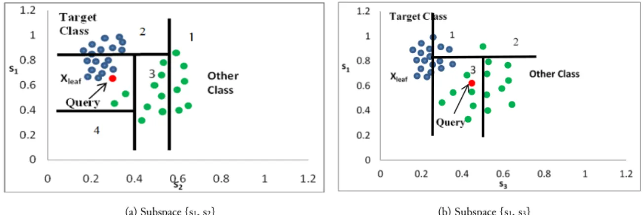
An simple illustration of the working mechanism of the tree-based likelihood contrast scoring measure of two dimensional subspaces {s1, s2} and {s1, s3} is given in Fig.1. The red point represents a query point while the blue points and the green points are the target objects and the other objects respectively. Each subspace space is splitted into two nodes and the process repeats on only node containing the query point until the minimum number of objects threshold is met. The splits are illustrated as the numbered horizontal or vertical lines. For subspace {s1, s2} (Fig. 1(a)), the sequence of the splitting operations are {1.vertical split-retaining left half-space}→{2.horizontal split-retaining

bottom half-space}→{3.vertical split-retaining left half-space}→{4.vertical split-retaining top

half-space}.Similarly, for subspace {s1, s3} in Fig. 1(b), recursive splits are needed to partition the subspace

(5)

Vol. 5, No. 2, July 2019, pp. 169-178

computed. The subspace {s1, s2} is identified as the contrast subspace because the query object falls in

the leaf node (Xleaf) which has higher number of target objects than the other objects.

(a) Subspace {s1, s2} (b) Subspace {s1, s3}

Fig. 1.Tree-based likelihood contrast scoring measure illustration. 2.2.The Framework of Tree-Based Mining Contrast Subspace Method

The number of possible subspaces that can be derived increases exponentially with the number of dimensions in the data set. This makes it practically impossible to calculate the likelihood contrast score of each subspace for a query object. Feature selection has been widely used in data mining tasks due to its capability of accelerating the mining process by reducing the dimensionality of data and improves the mining accuracy through eliminating the irrelevant features [16]–[19]. Hence, feature selection is applied to identify a subset of relevant one-dimensional subspaces from the full dimensional features given in the data set for searching contrast subspaces process. Accordingly, the tree-based contrast subspace mining method consists of two main phases which are the feature selection and the contrast subspace search. This proposed method is different from the existing methods as it is designed to find contrast subspace based on the objects in a group which share similarcharacteristics with the given query object in a subspace space. The framework of this tree-based mining method is shown in Fig. 2.

Fig. 2. Framework of tree-based mining contrast subspace method.

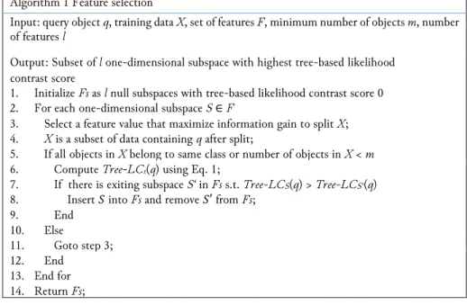
Algorithm 1 (Fig. 3) shows the pseudo-code of feature selection in phase one. In phase one, each one-dimensional subspace given in the data set are accessed on the basis of their likelihood contrast score with respect to a query object using (1). However, at this phase, it is noting that only discriminating feature values are selected for splitting data upon estimating the likelihood contrast score. A discriminate

(6)

Vol. 5, No. 2, July 2019, pp. 169-178

feature value is good on distinguishing objects from different classes so as to ensure objects of different classes are well separable in each node. The most common split criterion measure called information gain (info gain) is used to access how much information a feature value gives about the class [20]–[23]. Let consider the data set in a node X is splitted into node X1 and X2 using a feature value a. The info gain of the feature value a is shown as following

𝐼𝐼𝐼𝐼𝐼𝐼𝐼𝐼𝐼𝐼𝐼𝐼𝐼𝐼𝐼𝐼(𝐼𝐼) =𝐼𝐼𝐼𝐼𝐼𝐼𝐼𝐼(𝑋𝑋)− 𝐼𝐼𝐼𝐼𝐼𝐼𝐼𝐼𝑋𝑋(𝑋𝑋) (3)

where

𝐼𝐼𝐼𝐼𝐼𝐼𝐼𝐼(𝑋𝑋) =− ∑𝑗𝑗𝑖𝑖=1((𝐼𝐼𝑓𝑓𝑓𝑓𝑓𝑓(𝐶𝐶𝑖𝑖 ,𝑋𝑋)/|𝑋𝑋|) ∙ 𝑙𝑙𝐼𝐼𝑙𝑙2(𝐼𝐼𝑓𝑓𝑓𝑓𝑓𝑓(𝐶𝐶𝑖𝑖,𝑋𝑋)/|𝑋𝑋|)) (4) and

𝐼𝐼𝐼𝐼𝐼𝐼𝐼𝐼𝑋𝑋(𝑋𝑋) =−(((|𝑋𝑋1|)/|𝑋𝑋|) ∙ 𝐼𝐼𝐼𝐼𝐼𝐼𝐼𝐼(𝑋𝑋1)) + ((|𝑋𝑋2|)/|𝑋𝑋|) ∙ 𝐼𝐼𝐼𝐼𝐼𝐼𝐼𝐼(𝑋𝑋2))) (5)

where 𝐼𝐼𝑓𝑓𝑓𝑓𝑓𝑓(𝐶𝐶𝑖𝑖,𝑋𝑋) is the number of objects in node 𝑋𝑋 that belong to class 𝐶𝐶𝑖𝑖, 𝑗𝑗 is the number of

possible classes, |𝑋𝑋| is the number of objects in node 𝑋𝑋, and |𝑋𝑋𝑖𝑖| is the number of objects in node Xi

and 𝐼𝐼 is the number of nodes after the partition.

A discriminating feature value often gives maximal info gain. The assessment begins with sorting the values of a feature being considered in ascending order. This is followed by computing the info gain using (3) for each mid-value of every two subsequent values. The feature value with maximum info gain then is selected to split the data. After finished examining all features, the top l ranked one-dimensional subspaces in their likelihood contrast score are selected as a subset of relevant one-dimensional subspaces for contrast subspaces search in phase two. The parameter l is a user-determined number of one-dimensional subspaces.

Algorithm 1 Feature selection

Input: query object q, training data X, set of features F, minimum number of objects m, number of features l

Output: Subset of l one-dimensional subspace with highest tree-based likelihood contrast score

1. Initialize Fs as l null subspaces with tree-based likelihood contrast score 0 2. For each one-dimensional subspace S∈F

3. Select a feature valuethat maximize information gain to split X; 4. X is a subset of data containing q after split;

5. If all objects in X belong to same class or number of objects in X < m

6. Compute Tree-LCs(q) using Eq. 1;

7. If there is exiting subspace S‘ in Fs s.t. Tree-LCS(q) > Tree-LCS‘(q) 8. Insert 𝑆𝑆 into Fs and remove 𝑆𝑆′ from Fs;

9. End 10. Else 11. Goto step 3; 12. End 13. End for 14. Return Fs;

Fig. 3. Feature selection algorithm.

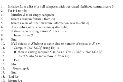
In phase two, random half binary trees are constructed by using the subset of selected dimensional subspaces. At this time, features are randomly selected from the subset of relevant one-dimensional subspaces to split data space repeatedly until it meets the stopping criterion such as mentioned in the previous section. Nevertheless, info gain is used to find the best splitting value of the features. The likelihood contrast score using (1) then is calculated. This is performed for t number of random half binary trees. Lastly, the top k highly scored trees are selected and the unique features in

(7)

Vol. 5, No. 2, July 2019, pp. 169-178

the corresponding trees are used as the contrast subspaces of the query object. This procedure of contrast subspace search is shown in Algorithm 2 (Fig. 4).

Algorithm 2 Contrast subspace search

Input: query object q, training data X, set of relevant one-dimensional subspace Fs, minimum number of objects m, number of subspaces k, number of trees t

Output: k contrast subspaces with highest tree-based likelihood contrast score

1. Initialize LS as a list of k null subspaces with tree-based likelihood contrast score 0 2. For i=1 to t do

3. Initialize S as an empty subspace; 4. Select a random feature s from Fs;

5. Select a value of s that maximize information gain to split X; 6. X is a subset of data containing q after split;

7. If there is no existing feature s‘ in S s.t. s'=s

8. Insert 𝑠𝑠 into S; 9. End

10. If all objects in X belong to same class or number of objects in X < m

11. Compute Tree-LCs(q) using Eq. 1;

12. If there is exiting subspace S‘ in LS s.t. Tree-LCS(q) > Tree-LCS‘ (q) 13. Insert S into LS and remove S' from LS;

14. End 15. Else 16. Goto step 4; 17. End 18. End for 19. Return LS;

Fig. 4.Contrast subspace search algorithm.

3. Results and Discussion

An experiment is conducted to evaluate the effectiveness of the proposed tree-based method. Since CSMiner-BPR is an extension of CSMiner, the proposed method is compared with the CSMiner-BPR only. The minimum number of objects threshold for leaf node m=25%, of total object in the data, the number of top ranked features l=4 and the number of random half binary trees t=100, which are found to perform well in finding contrast subspaces are used in this experiment. The experiments analysis for determining these best parameters setting is not included in this paper due to space limitation. While for CSMiner-BPR, the minimum likelihood threshold is set to 0.001 as suggested in their work [8]. The proposed and the existing method are implemented in Matlab 9.2 programming language.

Unfortunately, there is no ground truth of contrast subspace provided in real world data sets. Therefore, as the contrast subspace can be used to explain the separability of two classes, the accuracy of contrast subspaces is evaluated in term of how well the classes are separated (i.e. classification accuracy) in the contrast subspace projection. Four real world data sets obtained from UCI machine learning repository which have been used as benchmark in recent works are used [24]. All non-numerical features and all objects having missing values are removed from the data sets. The first data set are the Breast Cancer Wisconsin (BCW) data consisting of 699 clinical cases and is described by nine features of cell characteristics. Those cases are being classified to two classes {benign, malignant}. The second data set are the Wine data which contains 178 instances of chemical analysis results of three classes of wine. Each instance is described by 13 features which are derived from the constituents found in wines. The third data set are the Pima Indian Diabetes (PID) data which has 768 medical details of Pima Indian patients aged at least 21 years old and eight features obtained from certain diagnostic measurements. Those patients are being classified either positive diabetes or negative diabetes. Lastly, the fourth data set are Glass Identification (Glass) data consisting 214 samples of glass each with nine features correspond to glass composition. Each glass is classified into one of seven types of glass which comprised of building

(8)

Vol. 5, No. 2, July 2019, pp. 169-178

windows float processed, building windows non-float processed, vehicle windows float processed, vehicle windows non-float processed, containers, tableware, or headlamps.

The experiment on real world data sets is conducted as follows. For each data set, a class is taken as a target class and the remaining classes as other class. All objects that belong to the target class are taken as query objects. The proposed and the exiting methods are applied on all query objects to find their contrast subspaces. Herein, only the top one ranked contrast subspace is taken. These processes repeat by taking other class as target class and the rest of the classes as other class. Then, new data set consist of two classes which are labelled as Class A and Class B is generated for the contrast subspace of each query object. Class A contains the query object and the target objects which their distance is less or equal than the k-distance of a query object. According to related existing studies, they have shown that small fraction of data k=35, is sufficient for better performance [25]. The same value of k is employed in this experiment. This is performed to find a group of target objects that share similar characteristics with the query object. Objects from other class are random sampled to form Class B. The data size of Class B is same with Class A in order to avoid imbalance class which might affect the performance of the classification task. After that, the new data set are pumped into three classifiers, J48 (decision tree) [26], NB (naive bayes) [27], and SVM (support vector machine) [28], in WEKA to perform classification.

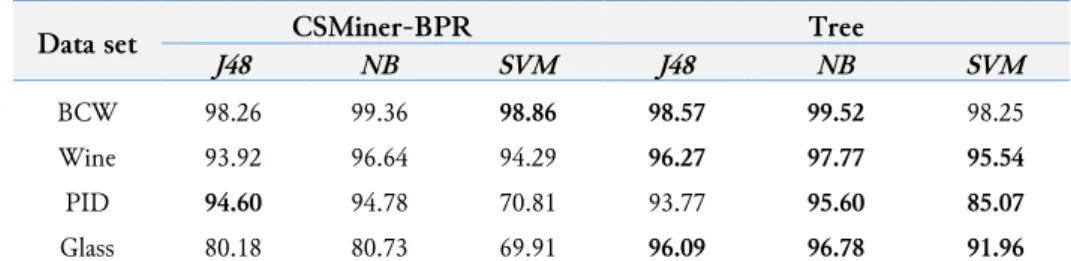
The average of classification accuracy percentage based on 10-fold cross validation of all query objects is used to measure the accuracy of the contrast subspace obtained for the query. The higher the classification accuracy, the more likely that contrast subspace is the right contrast subspace for the query object. Table 1 shows the experiment results of all classifiers on four real world data sets.

Table 1. Average classification accuracy (%) on four real world data sets.

Data set _J48 CSMiner-BPR _NB _SVM _J48 Tree _NB _SVM

BCW 98.26 99.36 98.86 98.57 99.52 98.25

Wine 93.92 96.64 94.29 96.27 97.77 95.54

PID 94.60 94.78 70.81 93.77 95.60 85.07

Glass 80.18 80.73 69.91 96.09 96.78 91.96

As depicted in Table 1, the proposed method with classifier J48 has higher average classification accuracy than the existing method with J48 on BCW, Wine, and Glass data. The proposed method with classifier NB shows higher average classification accuracy for all four data sets. In addition, the proposed method with SVM gives high average classification accuracy compared to the existing method on Wine, PID, and Glass data. Overall, the proposed method outperforms the existing method on ten out of twelve variety cases. This superior performance shows that the proposed method is able to find contrast subspaces of query objects. It also performs well compared to the existing method on mining contrast subspaces. This is because the proposed method employed the notion of divide-and-conquer which makes the mining process is not affected by the dimensionality of subspaces.

On the whole, the existing method produces better accuracy on only two out of nine cases. This poor performance from the fact that the dimensionality biased of density-based scoring measure causes the mining quality deteriorates [29], [30]. Hence, the empirical studies show that the proposed tree-based method demonstrates good performance in mining contrast subspaces of given query objects on real world data sets.

4. Conclusion

In this paper, a novel tree-based method has been proposed for mining contrast subspaces of a given query object in multidimensional numerical data set of two classes. The tree-based likelihood score does not involve distance computation in measuring the similarity between objects, thus, it does not have the dimensionality of subspaces biased issue. The tree-based likelihood contrast score of different dimensionalities of subspaces are comparable. Using the proposed tree-based method, the contrast

(9)

Vol. 5, No. 2, July 2019, pp. 169-178

subspaces of query object can be mined effectively regardless of the dimensionality of subspaces. In order to avoid exhaustive subspace search, feature selection has been applied which finds a subset of most relevant one-dimensional subspaces as an input feature space for further contrast subspaces search process. An extensive experiment has been carried out to evaluate the effectiveness of the proposed method and compared to the existing method. The empirical studies showed that the proposed method was capable to find contrast subspaces for the given query objects and performed better on several real world data sets specifically on ten out of twelve cases. As future work, an evolutionary algorithm will be exploited to optimize the contrast subspace search and the proposed method will be extended to mixed data set contain numerical and categorical values.

References

[1] X. H. Dang, B. Micenková, I. Assent, and R. T. Ng, “Local Outlier Detection with Interpretation,” 2013, pp. 304–320, doi: 10.1007/978-3-642-40994-3_20.

[2] T. Sellam and M. Kersten, “Fast, Explainable View Detection to Characterize Exploration Queries,” in Proceedings of the 28th International Conference on Scientific and Statistical Database Management - SSDBM ’16, 2016, pp. 1–12, doi: 10.1145/2949689.2949692.

[3] G. Manco, E. Ritacco, P. Rullo, L. Gallucci, W. Astill, D. Kimber, and M. Antonelli, “Fault detection and explanation through big data analysis on sensor streams,” Expert Syst. Appl., vol. 87, pp. 141–156, Nov. 2017, doi: 10.1016/j.eswa.2017.05.079.

[4] M. A. Siddiqui, A. Fern, T. G. Dietterich, and W.-K. Wong, “Sequential Feature Explanations for Anomaly Detection,” ACM Trans. Knowl. Discov. Data, vol. 13, no. 1, pp. 1–22, Jan. 2019, doi: 10.1145/3230666. [5] F. Angiulli, F. Fassetti, and L. Palopoli, “Detecting outlying properties of exceptional objects,” ACM Trans.

Database Syst., vol. 34, no. 1, pp. 1–62, Apr. 2009, doi: 10.1145/1508857.1508864.

[6] L. Duan, G. Tang, J. Pei, J. Bailey, A. Campbell, and C. Tang, “Mining outlying aspects on numeric data,” Data Min. Knowl. Discov., vol. 29, no. 5, pp. 1116–1151, Sep. 2015, doi: 10.1007/s10618-014-0398-2. [7] L. Duan, G. Tang, J. Pei, J. Bailey, G. Dong, A. Campbell, and C. Tang, “Mining Contrast Subspaces,”

2014, pp. 249–260, doi: 10.1007/978-3-319-06608-0_21.

[8] L. Duan, , G. Tang, J. Pei, J. Bailey, G. Dong, V. Nguyen, and C. Tang, “Efficient discovery of contrast subspaces for object explanation and characterization,” Knowl. Inf. Syst., vol. 47, no. 1, pp. 99–129, Apr. 2016, doi: 10.1007/s10115-015-0835-6.

[9] A. Zimek, E. Schubert, and H.-P. Kriegel, “A survey on unsupervised outlier detection in high-dimensional numerical data,” Stat. Anal. Data Min., vol. 5, no. 5, pp. 363–387, Oct. 2012, doi: 10.1002/sam.11161. [10] I. Assent, R. Krieger, E. Müller, and T. Seidl, “DUSC: Dimensionality Unbiased Subspace Clustering,” in

Seventh IEEE International Conference on Data Mining (ICDM 2007), 2007, pp. 409–414, doi:

10.1109/ICDM.2007.49.

[11] S. B. Kotsiantis, “Decision trees: a recent overview,” Artif. Intell. Rev., vol. 39, no. 4, pp. 261–283, Apr. 2013, doi: 10.1007/s10462-011-9272-4.

[12] C. C. Aggarwal, “Data Classification,” Data mining: the textbook, Springer, 2015, pp. 285–344, doi:

10.1007/978-3-319-14142-8_10.

[13] J. R. Quinlan, “Learning decision tree classifiers,” ACM Comput. Surv., vol. 28, no. 1, pp. 71–72, Mar. 1996, doi: 10.1145/234313.234346.

[14] Z.-H. Zhou, K.-J. Chen, and H.-B. Dai, “Enhancing relevance feedback in image retrieval using unlabeled data,” ACM Trans. Inf. Syst., vol. 24, no. 2, pp. 219–244, Apr. 2006, doi: 10.1145/1148020.1148023. [15] F. Laguzet, A. Romero, M. Gouiffès, L. Lacassagne, and D. Etiemble, “Color tracking with contextual

switching: real-time implementation on CPU,” J. Real-Time Image Process., vol. 10, no. 2, pp. 403–422, Jun. 2015, doi: 10.1007/s11554-013-0358-x.

[16] V. Bolón-Canedo, N. Sánchez-Maroño, and A. Alonso-Betanzos, Feature Selection for High-Dimensional Data, 2015, doi: https://doi.org/10.1007/978-3-319-21858-8.

(10)

Vol. 5, No. 2, July 2019, pp. 169-178

[17] G. Chandrashekar and F. Sahin, “A survey on feature selection methods,” Comput. Electr. Eng., vol. 40, no. 1, pp. 16–28, Jan. 2014, doi: 10.1016/j.compeleceng.2013.11.024.

[18] J. Li, K. Cheng, S. Wang, F. Morstatter, R. P. Trevino, J. Tang, and H. Liu, “Feature Selection: A Data Perspective,” ACM Comput. Surv., vol. 50, no. 6, pp. 1–45, Dec. 2017, doi: 10.1145/3136625.

[19] J. Tang and H. Liu, “Feature Selection for Social Media Data,” ACM Trans. Knowl. Discov. Data, vol. 8, no. 4, pp. 1–27, Oct. 2014, doi: 10.1145/2629587.

[20] N. Bhargava, G. Sharma, R. Bhargava, and M. Mathuria, “Decision tree analysis on j48 algorithm for data mining,” Proc. Int. J. Adv. Res. Comput. Sci. Softw. Eng., vol. 3, no. 6, 2013, available at: Google Scholar. [21] Z. Yu, F. Haghighat, B. C. M. Fung, and H. Yoshino, “A decision tree method for building energy demand

modeling,” Energy Build., vol. 42, no. 10, pp. 1637–1646, Oct. 2010, doi: 10.1016/j.enbuild.2010.04.006. [22] D. Lavanya and K. U. Rani, “Performance Evaluation of Decision Tree Classifiers on Medical Datasets,” Int.

J. Comput. Appl., vol. 26, no. 4, pp. 1–4, Jul. 2011, doi: 10.5120/3095-4247.

[23] E. Venkatesan and T. Velmurugan, “Performance Analysis of Decision Tree Algorithms for Breast Cancer Classification,” Indian J. Sci. Technol., vol. 8, no. 29, Nov. 2015, doi: 10.17485/ijst/2015/v8i1/84646. [24] C. Blake, “UCI repository of machine learning databases,” 1998, available at:

http://www.ics.uci.edu/~mlearn/MLRepository.html.

[25] B. Micenkova, R. T. Ng, X.-H. Dang, and I. Assent, “Explaining Outliers by Subspace Separability,” in 2013 IEEE 13th International Conference on Data Mining, 2013, pp. 518–527, doi: 10.1109/ICDM.2013.132. [26] J. Ali, R. Khan, N. Ahmad, and I. Maqsood, “Random forests and decision trees,” Int. J. Comput. Sci. Issues,

vol. 9, no. 5, p. 272, 2012, available at: Google Scholar.

[27] I. Rish, “An empirical study of the naive Bayes classifier,” in IJCAI 2001 workshop on empirical methods in artificial intelligence, 2001, vol. 3, no. 22, pp. 41–46, available at: Google Scholar.

[28] S. R. Gunn, “Support vector machines for classification and regression,” ISIS Tech. Rep., vol. 14, no. 1, pp. 5–16, 1998, available at: Google Scholar.

[29] H. V. Nguyen, V. Gopalkrishnan, and I. Assent, “An Unbiased Distance-Based Outlier Detection Approach for High-Dimensional Data,” 2011, pp. 138–152, doi: 10.1007/978-3-642-20149-3_12.

[30] I. Assent, R. Krieger, E. Müller, and T. Seidl, “EDSC: efficient density-based subspace clustering,” in Proceeding of the 17th ACM conference on Information and knowledge mining - CIKM ’08, 2008, p. 1093, doi: