APPENDIX 3
METHODS TO QUANTIFY THE PARAMETERS APPLIED IN THE RMi
"If no collective system and method exists, so much detail is usually recorded as to obscure the essential data needed for design."
Douglas A. Williamson and C. Rodney Kuhn (1988)
From Chapter 2 on data collection it has been shown that some of the uncertainties and errors in rock engineering stem from the rock mass characterizations, such as:
- The way the description is performed, or the quality of the characterization made of the various parameters in rock masses. As most of the input parameters in rock engineering and rock mechanics are found from observations, additional errors may be introduced from poorly defined descriptions and methods for data collection.
- During the measurements of joints and jointing, as the joints exposed only may be a portion of the joints considered to be representative of the entire rock mass.
This appendix has been worked out to remedy some of these tasks giving supplementary descriptions of the various methods in use to find the numerical values of the RMi parameters, either directly from measurements or observations, or from other types of measurements of rock strength properties or jointing features. Some of the methods described are time-consuming and expensive. Therefore, the methods used during collection of the field and laboratory investigations should be chosen to meet the requirements to accuracy and quality of the input data which may be determined by:
− the purpose and use of the construction;
− the stage of planning;
− the method of excavation;
− the availability to observe or measure the actual properties of the rock mass;
− the complexity of the geology; and
− the quality of the ground with respect to the type and use of the actual opening or the method of excavation.
For exchange of engineering geological data and for information to other people involved,
additional documentation of the rock mass conditions is important. Therefore, a verbal description should be included in the characterization. It should describe the composition and structure of the rock mass with special emphasis on the parameters of importance for engineering properties, including how the rock masses are related to the geological setting in the area. Important during the development of the RMi system has been to:
− group the rock masses in such a way that those parameters which are of most universal concern are clearly dealt with, and at the same time
− keeping the number of such parameters to a useful minimum. Thus, the input parameters selected, which are determined numerically in this appendix, are only:
− the uniaxial compressive strength of intact rock;
− the joint characteristics given as the joint condition factor; and
1 METHODS TO DETERMINE THE UNIAXIAL COMPRESSIVE STRENGTH OF ROCKS
For some engineering or rock mechanical purposes the numerical characterization of rock material alone can be used, for example boreability, aggregates for concrete, asphalt etc. Also in assessment for the use of fullface tunnel boring machines (TBM) rock properties such as compressive strength, hardness, anisotropy are often among the most important parameters. For stability evaluations and rock support engineering, however, the rock properties are mainly of importance only where they are weak or overstressed. Though rock properties in many cases are overruled by the effects of joints, it should be brought in mind that their properties highly determine how the joints have been formed, which in turn may explain their characteristics.
Although the geological classification of rocks is mainly based on formation and composition of the material, it is so well established that other methods for division of this material have not come into major use. Since, in rock mechanics and rock engineering, the rock behaviour rather than its
composition is of main importance Goodman (1989) has presented the classification shown in Table A3-1.
TABLE A3-1 BEHAVIOURAL CLASSIFICATION OF ROCKS (from Goodman, 1989)
GROUPS OF ROCKS Examples
I Crystalline texture
A. Soluble carbonates and salts ... B. Mica or other planar minerals in continuous bands ... C. Banded silicate minerals without continuous mica sheets
... D. Randomly oriented and distributed
silicate minerals of uniform grain size ... E. Randomly oriented and distributed silicate minerals in a
background of very fine grain and with vugs ... F. Highly sheared rocks ...
II Clastic texture
A. Stably cemented ... B. With slightly soluble cement ... C. With highly soluble cement ... D. Incompletely or weakly cemented ... E. Uncemented ...
III Very fine-grained rocks
A. Isotropic, hard rocks ... B. Anisotropic on a macro scale, but
microscopically isotropic hard rocks ... C. Microscopically anisotropic hard rocks ... D. Soft, soil-like rocks ...
IV Organic rocks A. Soft coal B. Hard coal C. 'Oil shale' D. Bituminous shale E. Tar sand
Limestone, dolomite, marble, rock salt, gypsum Mica schist, chlorite schist, graphite schist Gneiss
Granite, diorite, gabbro, syenite Basalt, rhyolite, other volcanic rocks Serpentinite, mylonite
Silica-cemented sandstones and limonite sandstones Calcite-cemented sandstone and conglomerate Gypsum-cemented sandstones and conglomerates Friable sandstone, tuff
Clay-bound sandstones
Hornfels, some basalts Cemented shales, flagstones Slate, phyllite
Compaction shale, chalk, marl
Lignite and bituminous coal
A verbal description of the rock should, in addition to the rock name and its strength, include possible anisotropy, weathering, and reduced long-term resistance to environmental influence (durability). The description of the rock could also contain information on texture, colour, lustre, small scale folds, etc. which can give information to a better understanding of the rock conditions as well as the jointing.
As rocks are composed of an aggregate of several types of minerals with different properties, arrangement and "welding", there are many factors which determine their strength properties. In addition, possible weathering and alteration can highly influence on the final strength properties of a rock. The effect of this is outlined in Section 1.6.4
Some minerals have a stronger influence on the properties of a rock than other. In rock construction the mica and similar minerals have an important contribution where they occur as parallel oriented continuous layers (Selmer-Olsen, 1964). Mica schists and phyllites with a high amount of mica show, therefore, strongly anisotropic properties which often influence in rock construction works as shown in Section 1.6.3.
1.1 The uniaxial compressive strength (σc )
In rock mechanics and engineering geology the boundary between rock and soil is defined in terms of the uniaxial compressive strength and not in terms of structure, texture or weathering. Several classifications of the compressive strength of rocks have been presented, as seen in Fig. A3-1. In this work a material with the strength ≤ 0,25 MPa is considered as soil, refer to ISRM (1978) and Table A3-1. 700 700 100 100 10 10 1 1
Very weak Weak Strong Very strong Coates
1964
Deere and Miller 1966
Geological Society 1970
Broch and Franklin 1972 Jennings 1973 Bieniawski 1973 ISRM 1979 Very low strength Low
strength Medium strength High strength Very high strength
Very weak Weak Moderately weak Moderately streng Strong Very strong Extremely strong Soil Rock Very low strength Low strength Medium strength High strength Very high strength Extremely high strength Very soft
rock Soft rock
Hard rock
Very hard
rock Extremely hard rock
Very low strength strengthLow Medium strength
High strength
Very high strength
Very low Low strength Moderate Medium High Very high Soil Soil Extremely low strength 0.7 0.7 0.5 0.5 2 2 3 3 4 4 5 5 6 6 7 7 8 8 20 20 30 30 40 40 50 50 70 70 200 200 300 300 400 400
Uniaxial compressive strength, MPa
Fig. A3-1 Various strength classifications for intact rock (from Bieniawski, 1984)
The uniaxial compressive strength can be determined directly by uniaxial compressive strength tests in the laboratory, or indirectly from point-load strength test (see Section 1.4.2). The tests should be carried out according to the methods recommended by the ISRM (1972).
The classification of the uniaxial compressive strength suggested by ISRM is shown in Tables A3-1a and A3-7.
TABLE A3-1a CLASSIFICATION OF THE UNIAXIAL COMPRESSIVE STRENGTH OF ROCKS (σc ) (from ISRM (1978)
---
Soil σc < 0.25 MPa
Extremely low strength σc = 0.25 - 1 MPa
Very low strength σc = 1 - 5 MPa
Low strength σc = 5 - 25 MPa
Medium strength σc = 25 - 50 MPa
High strength σc = 50 - 100 MPa
Very high strength σc = 100 - 250 MPa
Extremely high strength σc > 250 MPa
---
The uniaxial compressive strength of the rock constitutes the highest strength limit of the actual rock mass. ISRM (1981) has defined the uniaxial strength of a rock to samples of 50 mm diameter. A rock is, however, a fabric of minerals and grains bound or welded together. The rock therefore includes microscopic cracks and fissures. Rather large samples are required to include all the components that influence strength. When the size of the sample is so small that relatively few cracks are present, the failure is forced to involve a larger part of new crack growth than in a larger sample. Thus the strength is size dependent. This scale effect of rocks has been a subject of
investigations over the last 30 to 40 years. Fig. A3-2 shows the results from various tests compiled by Hoek and Brown (1980) where the scale effect (for specimens between 10 and 200 mm) has been found as
σc = σc50 (50/d)0.18 eq. (A3-1)
where σc50 is for specimens of 50 mm diameter, and d is the diameter (in mm) of the actual sample.
Symbol Rock Tested by
Marble Limestone Granite Basalt Basalt-andesite lava Gabbro Marble Norite Granite Quartz diorite Mog Koifman Burchartz et al. Koifman Melekidze Ilnickaya Ilnickaya Bieniawski Hoskins & Horino Pratt et al. 1.3 1.2 1.1 (σ σc/ c50) = (50/d) 0.18 1.0 0.9 0.8 0.7 0 50 100 150 200 Specimen diameter d - mm 250 U n ia x ia l c o m p re s s iv e s tr e n g th o f s p e c im e n U n ia x ia l c o m p re s s iv e s tr e n g th o f 5 0 m m d ia m e te r s p e c im e n σc σ c 5 0 166 169 169 169 169 169 169 167 170 168
Fig. A3-2 Influence of specimen size upon the uniaxial compressive strength of intact rock. (from Hoek and Brown, 1980)
Wagner (1987) has later shown that 'samples' with diameter more than 2 metres follow the following similar equation:
σcf = σc50 (50/d) 0.2 eq. (A3-1a)
ISRM (1980) recommends that the uniaxial compressive strength of the rock material in an area is given as the mean strength of rock samples taken away from faults, joints and other discontinuities where the rock may be more weathered. When the rock material is markedly anisotropic in its strength, the value used in the RMi should correspond to the direction along which the smallest mean strength was found. However, in such cases it is usually of importance to record the uniaxial compressive strength also in other directions.
Many compressive strength tests are made on dry specimens. ISRM (1980) recommends that the samples should be tested at a water content pertinent to the problem to be solved. Because rocks are often much weaker for wet than for dry materials, it is important to inform about the moisture conditions. This is further discussed in Section 1.3.
The compressive strength
σ
c50 is used directly in calculation of RMi. The accuracy and quality of this measurement has been discussed by several writers, as different modes of failure occur during the tests (Lama and Vutukuri, 1978; Hoek and Brown, 1980; Farmerand Kemeny, 1992; among others). Undoubtably, compressive strength is the mostly used test on rock samples and the loading resembles often situations in the field.
The uniaxial compressive test is time-consuming and is also restricted to those relatively hard, unbroken rocks that can be machined into regular specimens. Although the strength classification is based on laboratory tests, it can be approximated by simple methods. An experienced person can make a rough five-fold classification of rock strength with a hammer or pick. Deere and Miller (1966) have shown that rock strength can be estimated with a Scmidt hammer and a specific gravity test with enough reliability to make an adequate strength characterization. According to Patching and Coates (1968) the rock strength can be quickly and cheaply estimated in the field, and more precision can be attained, if required, by laboratory tests. Also from a fully description of a rock including composition and possible anisotropy and weathering it may in many instances be possible to assess the strength. These matters are described in the following. The methods, their applications, test procedures etc. are not dealt with, merely how the results can be used.
1.2 Effect of saturation upon rock strength
It is known that the influence of water on the strength of rocks may be considerable. From the published papers no general expressions other than the fact that moisture may reduce the strength of rocks drastically, has been established. Salustowicz (1965) has found that the decrease by moisture in sandstones and shales can be 40% and 60% of the dry strength respectively. Colback and Wiid (1965) mention a decrease from dry to saturated in the order of 50% both for quartzitic shale and for quartzitic sandstone. Table A3-2 shows compilation of some published result between compressive strength for saturated versus dry specimens. Results from Ruiz (1966) in Table A3-2 shows that wet strength may be higher than dry probably caused by heterogeneity and possible error from few tests. This effect has also been observed by Broch (1979) for some very fine-grained rocks (basalt, black shale).
TABLE A3-2 EFFECT OF SATURATION UPON STRENGTH (worked out from Lama and Vutukuri, 1978, with data from Feda, 1966; Ruiz, 1966; Boretti-Onyszkiewicz, 1966)
---
Number of Saturated in %
rocks tested Rock type of dry strength
--- 5 basalt 45 - 116 2 diabase 92 - 125 1 dolomite 83 3 limestone 56 - 118 1 schist 48 3 gneiss 36 - 59 5 gneiss 88 - 112 2 granitic gneiss 68 - 85 4 granite 68 - 116 1 granulite 54 1 quartzite 80 1 sandstone 90
5 sandstone 67 – 87 tested normal to bedding
" 54 – 92 tested parallel to bedding
---TABLE A3-3 EFFECT OF MOISTURE CONTENT ON COMPRESSIVE STRENGTH (worked out from Lama and Vutukuri, 1978, based on data from Price, 1960, and Obert et al., 1946)
---
No. of Relative compressive strengths for various
rocks ROCK TYPE Moisture contents expressed as % of oven-dry
tested Oven-dry Air-dry Saturated
--- 5 sandstone 100 51 - 99 45 – 90 1 marble 100 99 95 1 limestone 100 96 83 1 granite 100 93 86 1 slate 100 94 80 --- 0 25 50 75 100 Water content (%) P o in t lo a d s tr e n g th , I ( M N /m ) 2 S ( 3 2 ) gabbro B gabbro A quartzdiorite gneiss amphibolite amphibolite marble Kota sandstone Jamrani sandstone Singrauli sandstone Jhingurta sandstone 90 80 70 60 50 40 30 20 10 0 0.0 0.4 0.8 1.2 1.6
Equilibrium moisture content, ml/g, %
U n ia x ia l c o m p re s s iv e s tr e n g th , M P a x x x x x x x x 20 15 10 5 gneiss Fig. A3-3 Left: Point-load strength as a function of water content in rock cores (from Broch, 1979).
Right: Variation in uniaxial compressive strength with equilibrium moisture content for sandstones (from Seshagiri Rao et al. 1987).
The results shown in Table A3-3 differ whether the samples have been oven-dried or air-dried. This effect may strengthen the variation published in many papers on the effect of water upon strength. Broch (1979) has shown in Fig. A3-3 that the main strength reduction generally takes place for water contents less than 25%. Also Seshagiri Rao et al. (1987) have found that the main strength reduction for sandstones takes place at low moisture content (Fig. A3-3)
Broch (1979) concludes that the strength reduction from water increases with increasing amount of dark minerals (biotite, amphiboles, pyroxenes) and for increasing schistosity (anisotropy), as seen in Fig. A3-4.
From this complex picture of the effect of moisture and saturation upon rock strength Lama and Vutukuri (1978) conclude that: "Moisture in the rocks has a very significant effect on compressive strength in many instances. Unless the values to be used for design purposes are corrected to in situ conditions, catastrophic failures can occur. Many times, saturated specimens are recommended for tests so that the values obtained are conservative."
POINT LOAD STRENGTH OF WATER SATURATED ROCKS IN PER CENT OF THE STRENGTH OF OVEN DRY ROCKS
FINEGRAINED NONPOROUS ROCKS
ACIDIC INTERMEDIATE PLUTONIC ROCKS
GNEISSES
BASIC PLUTONIC ROCKS
MICASCHISTS
50 60 70 80 90 100 110 TYPES AND GROUPS OF
ROCKS
Fig. A3-4 The effect of water on point load strength of various groups of rocks (from Broch, 1979)
It is, therefore, important that the conditions at which the rocks are tested, are reported. ISRM (1972, 1981) suggests that rock samples are stored in 50% humidity for 5 - 6 days before testing.
1.3 Compressive strength determined from the point-load strength
The principle of the point load strength test is that a piece of rock is loaded between two hardened steel points. Details on the measuring procedure are described by ISRM (1985), and the method is further dealt with in several textbooks and papers (Lama and Vutukuri, 1978; Hoek and Brown, 1980, among others).
Both Franklin (1970) and Bieniawski (1984) recommend the use of point load strength index (Is) for rock strength testing. The reason is that Is can be determined in the field on specimens without preparation, using simple portable equipment. Also Broch (1983) points out the great advantage using the point load strength test as it does not require machined specimen. As long as the influence of specimen size and shape are considered in the calculation of the strength index, any piece of rock, whether the surface is smooth or rough, can in principle be tested. Although tests on irregular
specimens appear to be crude, Wittke & Louis (1969) have shown that the results need be no less reproducible than those obtained in uniaxial compression.
1.3.1 The point load strength index (Is)
Greminger (1982) relates the test results, Is(50), to standard 50 mm thick samples; this has also been applied by ISRM (1985) in a revised edition of the 'Suggested Method for determining point load strength'. The point load strength test is a form of "indirect tensile" test, but is largely irrelevant to its primary role in rock classification and strength as a tensile characterization (ISRM, 1985). Is(50) is approximately 0.80 times the uniaxial tensile or Brazilian tensile strength.
Also from the point load strength test a strength anisotropy index (Ia(50)) can be measured (Broch, 1983) from the maximum and minimum strengths obtained normal to, and parallel to the weakness planes, respectively, of the rock, i.e. bedding, foliation, cleavage, etc.
TABLE A3-4 CLASSIFICATIONS OF THE POINT LOAD STRENGTH ( Is) ---
TERM Bieniawski (1984) Deere (1966)
--- very high strength Is > 8 MPa Is > 10 MPa
high Is = 4 - 8 MPa Is = 5 - 10 MPa medium Is = 2 - 4 MPa Is = 2.5 - 5 MPa low Is = 1 - 2 MPa Is = 1.25 - 2.5 MPa
very low Is < 1 MPa Is < 1.25 MPa
---As shown in Fig. A3-3 the point load strength varies with the water content of the specimens. ISRM (1985) mentions that the variations are particularly pronounced for water saturations below 25%. At water saturation above 50% the strength is less influenced by small changes in water content, so that tests in this water content range are recommended unless tests on dry rock are specifically required. 1.3.2 The correlation between Is and σc
Point load strength test may often replace the uniaxial compressive strength test as it is, when properly conducted, as reliable and much quicker to measure. Hoek and Brown (1980) are of the opinion that a reasonable estimate of the uniaxial compressive strength of the rock can be obtained by means of the point load test. Other authors (Greminger, 1982; Seshagiri Rao et al., 1987) have, however, found that correlations with uniaxial compressive strength using
σc = k × Is eq. (A3-2)
or σc = k50× Is50 (related to 50 mm thick samples) eq. (A3-2a)
are only approximate. They show that, though the factor k or k50 generally varies between 15 and 25 it may sometimes vary between 10 and 50 especially for anisotropic rocks, so that errors of up to 100% are possible in using an arbitrary ratio value to predict compressive strength from point load strength. The variation in k and k50 published in various papers on point load strength results is shown in Table A3-5.
Greminger (1982) found that estimation of uniaxial compressive strength of anisotropic rocks may lead to significant errors, which is documented in Fig. A3-5. Seshagiri Rao et al. (1987) found for sandstones that k50 = σc / Is50 varied with the strength of the rock according to the following:
k50 = 14 for σc = 80 MPa, k50 = 12 for σc = 43 MPa k50 = 14 for σc = 24 MPa, k50 = 11 for σc = 6 MPa
TABLE A3-5 THE VALUE OF k PRESENTED IN VARIOUS PAPERS
REFERENCE value of k
Franklin (1970) k = approx. 16 Broch and Franklin (1972) k = 24
Indian standard (1978) k = 22
Hoek and Brown (1980) k= 14 + 0.175 D *)
Greminger (1982) no general correlation, see Fig. A3-5
ISRM (1985) k50 = 20 - 25
Brook (1985) k50 = 22
Seshagiri Rao et al. (1987) no general correlation Hansen (1988) no general correlation Ghosh and Srivastava (1991) k50 = 16
*)
D is the diameter or thickness of the tested sample
They argued that no general relation can be established between σc and Is50 . Also Hansen (1988) is of the same opinion from numerous tests carried out at the Technical University of Norway. The trend, therefore, seems to be that the factor k or k50 is higher for strong rocks. Based on the results above it is suggested, where no other information is available, to use the values of k50 (related to standard thickness) presented in Table A3-6 in the correlation from point load strength to uniaxial compressive strength. Augen gneiss Ruhr sandstone Chiandone gneiss Nuttlar slate Loaded parallel Loaded perpendicular 10 5 0 50 100 150 200 σc(50) = 24 Is(50)
-Fig. A3-5 Relationship between uniaxial compressive strength and point load strength index (from Greminger, 1982) TABLE A3-6 SUGGESTED VALUE OF THE FACTOR k50 VARYING
WITH THE STRENGTH OF THE ROCK σc (MPa) Is 50 (MPa) k50 25*) - 50 1.8 - 3.5 14 50 - 100 3.5 - 6 16 100 - 200 6 - 10 20 > 200 > 10 25 *)
Bieniawski (1973) suggests that point load strength test are not carried out on rocks having compressive strength less than approximately 25 MPa.
1.4 Compressive strength estimated from Schmidt hammer rebound number
The Schmidt hammer is used for non-destructive testing of the quality of rocks and concretes. It measures the 'rebound hardness' of the tested material. The mechanism of operation is simple; a
plugger, released by a spring, impacts against the tested rock surface. The rebound distance of the plunger is read directly from a numerical scale.
Measurements of rock properties with the Schmidt hammer are based on an imperfectly elastic impact of two bodies, one of which is represented by the impact of the test hammer and the other by the surface of the tested rock (Ayday and Göktan, 1992). Schmidt hammer models are designed in different levels of impact energy, and the two types L and N are commonly adapted for rock property determinations. The type L has an impact energy of 0.735 Nm, 1/3 of that of Type N. ISRM (1978) suggests that the L hammer can be used for the testing of rocks which have uniaxial compressive strength in the range of approximately 20 - 150 MPa . ISRM (1978) has also given a complete test procedure including a chart for correlating Scmidt rebound hardness to uniaxial compressive strength.
1.5 Compressive strength assessed from simple field test
Sometimes, particularly at an early stage in the description of the rock mass, strength may be assessed without testing (ISRM, 1980). Such a first estimate of the uniaxial compressive strength (
σc) may be made by visual and sensory description of hardness of rock or consistency of a soil (Piteau, 1970; Herget, 1982). The strength can be judged from simple hardness tests in the field with geological pick by observing the resistance to breaking under impact, as shown in Table A3-7.
TABLE A3-7 SIMPLE FIELD IDENTIFICATION COMPRESSIVE STRENGTH OF ROCK AND CLAY (from ISRM, 1978)
Approx.
GRADE TERM FIELD IDENTIFICATION range of σc
(MPa)
S1 Very soft clay Easily penetrated several inches by fist. < 0.025
S2 Soft clay Easily penetrated several inches by thumb. 0.025-0.05
S3 Firm clay Can be penetrated several inches by thumb with moderate effort. 0.05 -0.10 S4 Stiff clay Readily intended by thumb, but penetrated only with great effort. 0.10 -0.25
S5 Very stiff clay Readily intended by thumbnail. 0.25 -0.50
S6 Hard clay Intended with difficulty by thumbnail. > 0.50
- - -
R0 Extremely weak rock Intended by thumbnail. 0.25 - 1
R1 Very weak rock Crumbles under firm blows with point of geological hammer; 1 - 5 can be peeled by a pocket knife.
R2 Weak rock Can be peeled by a pocket knife with difficulty, shallow identi- 5 - 25 fications made by firm blow with point of geological hammer.
R3 Medium strong rock Cannot be scraped or peeled with a pocket knife; specimen can 25 - 50 be fractured with single firm blow of geological hammer.
R4 Strong rock Specimen requires more than one blow of geological hammer 50 - 100 to fracture it.
R5 Very strong rock Specimen requires many blows of geological hammer to fracture it. 100 - 250 R6 Extremely strong rock Specimen can only be chipped with geological hammer. > 250
The clays in grade S1 - S6 can be silty clays and combinations of silts and clays with sands, generally slow draining.
The hammer test should be made with a geologist's hammer on pieces about 10 cm thick placed on a hard surface, and tests with the hand should be made on pieces about 4 cm thick. The pieces must not have incipient fractures, and therefore several should be tested.
For anisotropic rocks tests should be carried out in different directions to the structure. The lowest representative values should be applied. It is also possible to use the foliation anisotropy factor
described in Section 1.7.3 to find the lowest value of compressive strength to be applied in the RMi.
1.6 Compressive strength estimated from rock description
Probably the most generally used single describer of rock structure has been "rock type". In this term a wide variety of geological factors is embraced, ranging from basic rock origin: igneous, sedimentary and metamorphic, to special properties such as texture and structure, mineral size and composition, anisotropy, degree of alterations, etc.
According to Franklin (1970) over 2000 names are available for the igneous rocks that comprise about 25% of the earth's crust, in contrast to the greater abundance of mudrocks (35%) for which only a handful of terms exist; yet the mudrocks show a much wider variation in mechanical
behaviour and greater challenges in rock constructions. From the rock engineering point of view this vast amount of rock types can be grouped into a reduced number of about 40, regarding strength and behaviour.
Geological nomenclature emphasizes solid constituents whereas from the engineers' point of view pores, cracks and fissures are of greater mechanical significance. Petrological data can, however, make an important contribution towards the prediction of mechanical performance, provided that additional information on the anisotropy and weathering is provided.
In most instances, a simple hand-specimen name will likely be adequate to determine the rock type and name. An added term to indicate grain size may often be useful (Patching and Coates, 1968). For many rocks the name of the rock, its homogeneity and continuity can be established by visual observation in the field.
An accurate classification of rock materials used by geologists requires, however, often a detailed consideration of mineralogy and petrography for instance from thin section analysis, an
investigation, which may seldom be important to engineers only in few cases. 1.6.1 Main geological characteristics
The minerals of most igneous rocks are hard and may display cleavage but are of a dense interfingering nature resulting in homogeneous materials with only slight, if any, directional differences in mechanical properties of the rock.
The minerals of sedimentary rocks are usually softer and are of generally weaker assemblage than the igneous rocks. In these rocks the minerals are not interlocking but are cemented together with inter-granular matrix material. Sedimentary rocks usually contain lamination or other sedimentation structures and, therefore, may exhibit significant anisotropy in physical properties depending upon the degree of their development. Of this group, argillaceous and sandstone rocks are usually the most strongly anisotropic.
The metamorphic rocks, more particularly the micaceous and chloritic schists, are probably the most outstanding with respect to anisotropy. The metamorphism have resulted in harder minerals in most cases; however, the preferred orientation of platy minerals due to shearing movements results in considerable directional differences in mechanical properties. Rocks with gneissic texture are generally not strongly anisotropic. Slate, due to well developed slaty cleavage, is highly anisotropic.
1.6.2 Strength assessment from rock name
The rock types often give relative indications of their inherent properties (Piteau, 1970; Patching and Coates, 1968). For many rocks, however, the correlation between the petrographic names of rocks and their mechanical properties may be poor, caused by difference in composition, grain size, porosity, cementation, anisotropy within each type. Nevertheless, a great deal of associated
information about a rock can be inferred from its geological name, such as whether it may be homogeneous, layered, schistose or irregular.
TABLE A3-8 NORMAL RANGE OF COMPRESSIVE STRENGTH FOR SOME COMMON ROCK TYPES (data from Hansen, 1988 and Hoek and Brown, 1980) AND VALUES FOR THE m FACTOR IN HOEK-BROWN FAILURE CRITERION (from Hoek et al., 1992).
Rock name Uniaxial compressive strength σc Rating of the factor mi1) Rock name Uniaxial compressive strength σc Rating of the factor mi 1)
low average high low average high
Sedimentary rocks Anhydrite Coal Claystone Conglomerate Coral chalk Dolomite Limestone Mudstone Shale Sandstone Siltstone Tuff Igneous rocks Andesite Anorthosite Basalt Diabase (dolerite) Diorite Gabbro Granite Granodiorite Monzonite Nepheline syenite Norite Pegmatite Rhyolite Syenite
Ultra basic rock
120'? 16" 21" 26" 2' 5' 10' 70 85 100 3 10 18 60' 100'300' 50* 100' 180* 45 95 145 36" 95" 172" 75 120 160 10' 80' 180' 3' 25' 150' 75' 140' 300' 40 125 210 100 165 355" 227" 280" 319" 100 140 190 190 240 285 95 160 230 75 105 135 85 145 230 125 165 200 290" 298" 326" 39 50 62 85'? 75 150 230 80' 160 360 13.2 3.4 (20) 7.2 10.1 8.4 18.8 9.6 18.9 (17) 15.2 27 ? 25.8 32.7 20 ? 30 ? 21.7 (20) 30 ? Metamorphic rocks Amphibolite Amphibolitic gneiss Augen gneiss Black shale Garnet mica schist Granite gneiss Granulite Gneiss Gneiss granite Greenschist Greenstone Greywacke Marble Mica gneiss Mica quartzite Mica schist Mylonite Phyllite Quartz sandstone Quartzite Quartzitic phyllite Serpentinite Slate Talc schist 75 125 250 95 160 230 95 160 230 35 70 105 75 105 130 80 120 155 80' 150 280 80 130 185 65 105 140 65 75 85 120' 170* 280* 100 120 145 60' 130' 230' 55 80 100 45 85 125 20 80* 170* 65 90 120 21 50 80 70 120 175 75 145 245 45 100 155 65 135 200 120' 190' 300' 45 65 90 31.2 31 ? 30 ? 30 ? 29.2 30 ? 20 ? 9.3 30 ? 25 ? 15 ? 13 ? 23.7 11.4 10 ? Soil materials2):
Very soft clay σc = 0.025 MPa Soft clay σc = 0.025 - 0.05 MPa Firm clay σc = 0.05 - 0.1 MPa
Stiff clay σc = 0.1 - 0.25 MPa Very stiff clay σc = 0.25 - 0.5 MPa Hard clay σc = > 0.5 MPa
Silt, sand: assume σc = 0.0001- 0.001 MPa
* Values found by the Technical University of Norway, (NTH) Inst. for rock mechanics. ' Values given in Lama and Vutukuri, 1978.
1)
Refer to the factor, m, in the failure criterion for rock masses by Hoek et al. (1992), mi is the parameter for intact rock, see
Chapter 9, Section 1. Values in parenthesis have been estimated by Hoek et al (1992); some others with question mark have been assumed in this work.
2) For clays the values of the uniaxial compressive strength is based on ISRM (1978) as presented in Table A3-7.
A good description of the rock material is a prerequisite when such strength evaluations are made. Adjustments for possible anisotropy (schistosity, foliation, bedding) and weathering/alteration in rocks are further described in Section 1.7.3 and 1.7.4.
Where representative, fresh specimens of the various types occur, it is, however, often possible if not accurate values are required to make estimates of the compressive strength from the rock name as presented in Table A3-8. Additional results from compressive strength tests are given in many textbooks. Refer to Lama and Vutukuri (1978), Hoek and Brown (1980) etc. In the following some methods to estimate the uniaxial compressive strength for anisotropic and weathered or altered rocks are outlined.
1.6.3 Reduction in strength from anisotropy
Anisotropy in rock material is mainly caused by schistosity, foliation or bedding. The difference in properties is determined by the arrangement and amount of flaky and elongated minerals (mica, chlorite, amphiboles). This intrinsic rock property tends to be significant even at the scale of a laboratory test specimen.
Quartzitic phyllite Carbonaceous phyllite Micaceous phyllite Experimental Theoretical β (degrees) U n ia x ia l C o m p re s s iv e S tr e n g th (M P a ) 0 30 60 90 20 40 60 80 100 120 Single plane of weakness Multiple planes of weakness Case - Case - I II Case-I Case-II C o m p re s s iv e s tr e n g th , σ 1 β (degrees) (b) 0 30 60 90 Shearing Splitting σ2 = σ3 σ1 (a) β β
Fig. A3-6 Experimental and theoretical variation of uniaxial compressive strength with angle between schistosity plane and direction of testing (from Ramamurthy et al., 1993)
Tsidzi (1986, 1987, 1990) has presented results from tests on strength anisotropy in foliated rocks, together with measurements of their intrinsic anisotropic foliation fabric. The lowest strength value occurred when the orientation of the anisotropic fabric element (bedding, foliation) to the specimen loading axis was between 30o and 45o, and the highest value for orientation either 0o or 90o. This effect has also been shown by Ramamurthy et al., (1993) in Fig. A3-6, Hoek and Brown (1980) and many other authors. Hence, the estimation of compressive strength anisotropy of rocks in terms of values obtained only for tests parallel (0o) and normal (90o) to the foliation plan give only limited information on the rock strength.
From his tests carried out on slates, schists, and gneisses with compressive strength ranging between 20 and 285 MPa Tsidzi (1990) has worked out the classification which is shown in Table A3-9. From regressions Tsidzi arrived at the following expression for the uniaxial compressive strength anisotropy factor:
fA = 0.95 + 0.17 Fi eq. (A3-3)
where Fi is the foliation index. Its ratings are indicated in Table A3-9.
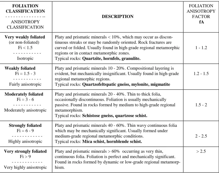
TABLE A3-9 CLASSIFICATION OF FOLIATION AND ANISOTROPY OF ROCKS (from Tsidzi, 1986, 1987, 1990) FOLIATION CLASSIFICATION - - - -- ANISOTROPY CLASSIFICATION DESCRIPTION FOLIATION ANISOTROPY FACTOR fA
Very weakly foliated (or non-foliated)
Fi < 1.5 - - -
Isotropic
Platy and prismatic minerals < 10%, which may occur as discon-tinuous streaks or may be randomly oriented. Rock fractures are curved or folded. Usually found in high-grade regional metamorphic regions or in contact metamorphic zones.
Typical rocks: Quartzite, hornfels, granulite.
1 - 1.2
Weakly foliated Fi = 1.5 - 3 - - - Fairly anisotropic
Platy and prismatic minerals 10 - 20%. Compositional layering is evident, but mechanically insignificant. Usually found in high-grade regional metamorphic regions.
Typical rocks: Quartzofeltspatic gneiss, mylonite, migmatite
1.2 - 1.5
Moderately foliated Fi = 3 - 6 - - - Moderately anisotropic
Platy and prismatic minerals 20 - 40%. Thin to thick folia, occasionally discontinuous. Foliation is usually mechanically passive. Found in rocks formed by medium to high-grade regional metamorphism.
Typical rocks: Schistose gneiss, quartzose schist.
1.5 - 2
Strongly foliated Fi = 6 - 9 - - - Highly anisotropic
Platy and prismatic minerals 40 - 60%. Thin wavy continuous folia which may be mechanically significant. Usually formed under medium-grade regional metamorphic conditions.
Typical rocks: Mica schist, hornblende schist.
2 - 2.5
Very strongly foliated Fi > 9
- - - Very highly anisotropic
Platy and prismatic minerals > 60% occurring as very thin, continuous folia. Foliation is perfect and mechanically significant. Found in rocks formed by dynamic or low-grade regional metamorp-hism.
Typical rocks: Slate, small folded phyllite.
Fi = foliation index
The foliation index can be found from thin section analysis by measuring the mineral composition and the shape of the minerals as presented by Tsidzi (1986).
From the values of fA in Table A3-9 combined with the content of platy and prismatic minerals, the following equation is found:
fA = 1 + 2.5 c/100 eq. (A3-4)
where c is the content of platy and prismatic minerals in % .
According to Tsidzi (1989), the strength anisotropy index fA is directly proportional to foliation regardless of the physical condition of rock. Thus, the minimum compressive strength of the foliated rock can roughly be assessed as
σc min = σc max /fA = σc max /(1 + 2.5 c/100) eq. (A3-5)
In their works on anisotropic rocks Sing et al. (1989) have introduced the anisotropy ratio is defined as Rc = σc 90 /σc min , where σc 90 is the uniaxial compressive strength measured at right angle to the schistosity or bedding. Their results shown in Table A3-10 indicate that the strength reduction caused by the anisotropy (Rc) is considerably higher than fA in Table A3-9.
TABLE A3-10 CLASSIFICATION OF ANISOTROPY
(from Sing et al., 1989 and Ramamurthy et al., 1993)
Anisotropy ratio Classification Rock types
Rc
1 - 1.1 Isotropic
1.11 - 2.0 Low anisotropy Shales 2.01 - 4.0 Medium anisotropy _ _
4.01 - 6.0 High anisotropy Slates > 6.0 Very high anisotropy _ Phyllites
A possible reason for this is that the rocks tested by Tsidzi generally exhibit stronger small scale foldings which will reduce the effect of the foliation. Also possible differences in moisture content may influence on the results. None of the authors have specified under which conditions the test were carried out.
The sonic velocity anisotropy coefficient for some rocks is presented in Table A3-11 , which shows values lower than the strength anisotropy factor of Tsidzi in Table A3-9.
TABLE A3-11 SONIC ANISOTROPY COEFFICIENTS FOR SOME ROCKS (from Lama and Vutukuri, 1978)
anisotropy | anisotropy
ROCK coefficient | ROCK coefficient
Vº/VÁ. | Vº/VÁ.
Austin chalk 1.17 | Anhydrites 1.12 - 1.16 Limestones 1.04 - 1.30 | Marl 1.10 Salt no anisotropy | Sandstones 1.0 - 1.19 Shales 1.07 - 1.40 | Gneisses 1.20 - 1.27 Mica schist 1.36 | Granodiorite 1.33 Serpentine 1.18 |
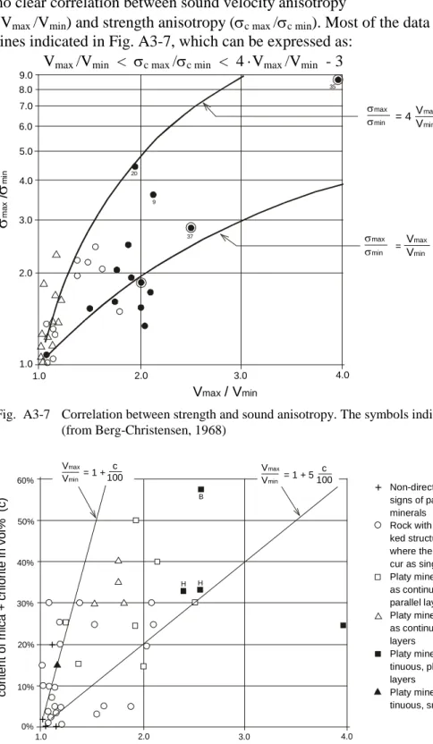
In an earlier work performed by Bergh-Christensen (1968) correlations between compressive strength anisotropy and wave velocity anisotropy were investigated. As shown in Fig. A3-7 there is no clear correlation between sound velocity anisotropy
(Vmax /Vmin) and strength anisotropy (σc max /σc min). Most of the data fall, however, within the to lines indicated in Fig. A3-7, which can be expressed as:
Vmax /Vmin < σc max /σc min < 4 ⋅Vmax /Vmin - 3 eq. (A3-6)
Vmax / Vmin σ σ m a x m in / 9.0 8.0 7.0 6.0 5.0 4.0 3.0 2.0 1.0 1.0 2.0 3.0 4.0 σ σ max min σ σ max min V V max min V V max min = 4 - 3 9 20 37 35 =
Fig. A3-7 Correlation between strength and sound anisotropy. The symbols indicate measured rock blasting indexes. (from Berg-Christensen, 1968) Vmax min/ V c o n te n t o f m ic a + c h lo ri te i n v o l% (c ) 1.0 2.0 3.0 4.0 60% 50% 40% 30% 20% 10% 0% H H B + + + + + Non-directional structure, no signs of parallel orientation of minerals
Rock with more or less ma-ked structural planaraty, where the platy minerals oc-cur as single grains Platy minerals occur partly as continuous, planar and parallel layers
Platy minerals occur partly as continuous, small-folded layers
Platy minerals as con-tinuous, planar and parallel layers
Platy minerals occur as con-tinuous, small-folded layers V V max min c 100 = 1 + V V max min c 100 = 1 + 5
Fig. A3-8 Correlation between content of flaky minerals (mica and chlorite) and sound velocity ratio for various textures of rock (from Berg-Christensen, 1968).
(In the groups with continuous layers of flaky minerals there are rocks that do not follow the average trend. One explanation can be that the classification into the structural groups are made from simple observations (personal communication with Bergh-Christensen, 1992))
In Fig. A3-8 showing the relation between the sonic velocity anisotropy and the content of flaky minerals it is seen that most data lies within the two lines represented by the following expression:
1 + c/100 < Vmax /Vmin < 1 + 5c/100 eq. (A3-7)
where V is the seismic velocity, and c is the content of flaky minerals (mica and chlorite) given in %.
By roughly combining the lowest with the highest values in eq. (A3-6) and eq. (A3-7) it is possible to find the rock anisotropy factor, fA, from the content of flaky minerals given as:
1 + 4c/100 < fA < 1 + 5c/100 eq. (A3-8)
This equation gives somewhat higher values for fA than eq. (A3-5) found by Tsidzi; for example, for 50% content of flaky minerals fA = 3 - 3.5 with eq. (A3-8), compared to Tsidzi's fA = 2.25. Eq. (A3-8) gives, however, lower values than Rc (see Table A3-10).
From the foregoing it is apparent that it is not a well defined, simple method to estimate the effect of anisotropy upon strength. The anisotropy factor varies with the method used, in addition the
definition of the anisotropy class seems to be very approximate as possible small-scale folding is not included. The method presented by Tsidzi in eq. (A3-5) seems, however to be better documented and may, therefore, be the best for rough estimates. More investigations and are required to arrive at better expressions for the rock anisotropy.
1.6.4 Reduction in strength from weathering and alteration
Weathering of rocks is a result of the destructive processes from atmospheric agents at or near the Earth's surface, while alteration is typically brought about by the action of hydrothermal processes. Both processes produce changes of the mineralogical composition of a rock, affecting colour, texture, composition, firmness or form; features that result in reduction of the mechanical properties of a rock. Deterioration from weathering and alteration generally affects the walls of the
discontinuities more than the interior of the rock (Piteau, 1970).
TABLE A3-12 ENGINEERING CLASSIFICATION OF THE WEATHERING OF ROCKS (from Lama and Vutukuri, 1978)
CLASSIFICATION DESCRIPTION
Unweathered No visible signs of weathering. Rock fresh, crystals bright. Few discontinuities may show slight staining.
Slightly Penetrative weathering developed on open discontinuity surfaces but only slight
weathered weathering of rock material. Discontinuities are discoloured and discoloration can extend into rock up to a few mm from discontinuity surface.
Moderately Slight discoloration extends through the greater part of the rock mass. the rock is not friable
weathered (except in the case of poorly cemented sedimentary rocks). Discontinuities are stained and/or contain a filling comprising altered materials.
Highly Weathering extends throughout rock mass and the rock material is partly friable. Rock
weathered has no lustre. All material except quartz is discoloured. Rock can be excavated with geologist's pick.
Completely Rock is totally discoloured and decomposed and in a friable condition with only fragments
weathered of the rock texture and structure preserved. The external appearance is that of a soil.
Residual soil Soil material with complete disintegration of texture, structure and mineralogy of the parent rock.
Characterization of the state of weathering or alteration both for the rock material and for the discontinuities is therefore an essential part of the rock parameters to be applied (ISRM, 1978). In rock engineering and construction it is seldom of interest to describe whether the process of
weathering or alteration has been acting; the main topic is to characterize the result. Knowledge of the processes, which have taken place, can however be important for the understanding and
interpretation of the geological conditions and of the condition of the rocks likely to be found. In general, the degree of weathering is usually estimated from visual observations, where only the qualitative information is required. Table A3-12 shows classification of weathering/alteration similar to that presented by ISRM (1978). A more precise characterization of alteration and weathering can be found from analysis of thin sections in a microscope.
Papadopoulos and Marinos (1992) have made tests on a wide variety of petrological rock types, consisting of clayey schists, phyllites, mica schists, sandstones with secondary anisotropy due to weathering from tectonic action. Some of their results are shown in Fig. A3-9 where the grade of weathering is according to the ISRM (1978) or the similar classification by Lama and Vutukuri (1978) in Table A3-12. I II III IV I II III IV MPa MPa 6 6 5 5 4 4 3 3 2 2 1 1 I Is (50) s (50) (a) (b) W.G. W.G.
Fig. A3-9 Correlation between weathering grade I - IV and point-load strength values Is50 (from Papadopoulos and
Marinos, 1992)
The reduction factor from weathering is found as the ratio Is50fresh /Is50 weathered in Fig. A3-9. Results from tests parallel and normal to anisotropy are shown in Table A3-13, in which also the rating of a rock weathering factor (fW) has been suggested. From this the point load strength of the weathered or altered rock can roughly be found as
Is50 = Is50 fresh /fW eq. (A3-9)
Assuming that the strength reduction for the compressive strength is similar it is approximately found from
σc = σc fresh /fW = k50 × Is50 fresh /fW eq. (A3-10)
The suggested rating of the weathering/alteration factor in Table A3-13 is, however, based on very few data and it is therefore considered very rough, especially for high grades of weathering. It should, therefore, mainly be applied for rough calculations before better strength data are available.
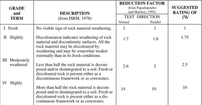
TABLE A3-13 SUGGESTED WEATHERING/ALTERATION FACTOR (fW) OF ROCKS, fW (worked out partly from ISRM (1978) and Papadopoulos and Marinos (1992).
GRADE and TERM DESCRIPTION (from ISRM, 1978) REDUCTION FACTOR (from Papadopoulos
and Marinos, 1992) SUGGESTED RATING OF fW TEST DIRECTION Normal Parallel I Fresh II Slightly III Moderately weathered IV Highly
No visible sign of rock material weathering. Discolouration indicates weathering of rock material and discontinuity surfaces. All the rock material may be discoloured by weathering and may be somewhat weaker externally than in its fresh conditions. Less than half the rock material is decom-posed and/or disintegrated to a soil. Fresh or discoloured rock is present either as a discontinuous framework or as corestones. More than half the rock material is decom-posed and/or disintegrated to a soil. Fresh or discoloured rock is present either as a dis-continuous framework or as corestones.
1 1 1.7 1.8 2.6 2 14 10 1 1.75 2.5 10 1.7 Summary
In addition to compression tests in laboratory the uniaxial compressive strength of the rock may be found from several other methods which have been shortly described. These are:
• Compressive strength estimated from the point-load strength (Is), given as
σc = k50 × Is50
where values of k50 varying with the rock strength related to 50 mm samples, have been suggested.
• Compressive strength found from the Schmidt hammer rebound number.
• Compressive strength assessed from simple field test using a geological hammer.
Where test data of the rock is not available the uniaxial compressive strength may be estimated from the geological rock name and additional information on its structure and weathering/alteration. For anisotropic and weathered/altered rocks a rough estimate of the uniaxial compressive strength can be found from
σc = σc50 /(fA × fW) eq. (A3-11)
where σc50 can be found for fresh rocks from published strength tables, and
fA, fW are the foliation anisotropy and weathering/alteration factors, respectively. Sug-gested ratings have been given for both factors, but additional investigations are required to improve these approximate values.
The lowest value (σc min) is applied in RMi. Therefore, it is important to check if the effect of anisotropy is included in σc50 . It is also important that the rock description - on which the estimates are based - clearly delineate the composition and structure of the rock, and that the applied terms and
characterizations of the rock are well defined. Further information on useful description of rocks is outlined in Section 5.
2 METHODS TO DETERMINE THE JOINT CONDITION FACTOR ( jC)
"The success of the of the field investigation will depend on the geologist's ability to recognise and describe in a quantitative manner those factors which the engineer can include in his analysis."
Douglas R. Piteau, 1970
The usually large number of joints with various conditions involved in a rock mass, cause that simplifications have to be made and that rapid and inexpensive measurements are preferred. The joint condition factor, jC, is meant to represent the main inherent variables of the friction properties of joints in a rock mass. Basically, the condition of joints are made up of the following parameters (see alt. A in Fig. A3-11):
• The roughness of the joint walls, given as the joint roughness factor (jR), similar to Jr in the Q-system. jR consists of:
- smoothness (or unevenness) of the joint wall surface, and - waviness (or planarity) of the joint wall plane.
• The character of the joint wall including possible filling and its thickness, expressed in the joint alteration factor (jA).1
• Length and continuity of the joints, expressed as the joint size factor, jL, which is considered a scale and geometry factor to mainly include the different importance between large, pervasive joints and small, irregular joints on rock mass behaviour.
Similar, as for the Jr/Ja in the Q system, the ratio jR/jA is roughly a function of tan φ, the peak friction coefficient of the joint. Thus, also measurements of the joint friction angle can be used to find the ratio jR/jA as shown in Fig. A3-12. This method (alt. B) is based on measurements of the joint roughness combined with input of the actual type and size of joints. Alt. A is based wholly on observations.
JOINT WAVINESS
JOINT SMOOTHNESS
JOINT CHARACTER
JOINT LENGTH AND TERMINATION JOINT LENGTH AND
TERMINATION BASIC FRICTION ANGLE ( Φb ) JOINT ROUGHNESS COEFFICIENT (JRC) JOINT TYPE & ROCK TYPE JOINT ROUGHNESS FACTOR ( jR ) DILATION ANGLE ( i ) JOINT SIZE FACTOR ( jL ) JOINT SIZE FACTOR ( jL ) JOINT ALTERATION FACTOR ( jA ) JOINT CONDITION FACTOR JOINT CONDITION FACTOR PEAK FRICTION ANGLE ( ) ( similar to jR/jA ) φ jC = jC = jR jA jR jA jL jL alternativ input field data field data
Fig. A3-11 The two main methods to find the joint condition factor, jC.
Alt. A is described in Section 2.1 and 2.2, alt. B in Section 2.3. The joint size factor, jL, which is used in both alternatives, is described in Section 2.4
2.1 Estimating the joint roughness factor (jR)
The roughness of joint walls is characterized by a large scale waviness and a small scale smoothness or unevenness, ISRM (1978), see Fig. A3-12. During shear displacement the waviness undulations, if locked and in contact, cause dilation since they are too large to be sheared off, while the
asperities of the smoothness tend to be damaged unless the joint walls are of high strength and/or the stress levels are low. In practice, it is seldom possible to observe and measure both these features along the entire joint. Some sort of simplification has therefore to be made as outlined in this section.
Fig. A3-12 The joint wall features can be characterized by the large scale waviness and the small scale smoothness (or unevenness).
2.1.1 Field measurements of large scale roughness
Accurate measurements of joint waviness in rock exposures is relatively time-consuming by any of the currently available procedures (Stimpson, 1982). The three most practical methods are:
1. To estimate the overall roughness (undulation) angle by taking measurements of joint
orientation with a Clar Compass to which the base plates of different dimensions are attached, see Fig. A3-13 left.
2. To measure the roughness along a limited part of the joint using a feeler or contour gauge to draw a profile of the surface, Stimpson (1982). Also Barton and Choubey (1977) makes use of this method especially in connection with core logging.
3. To reconstruct a profile of the joint surface from measurements of the distance to the surface from a datum (typically a rod or rule laid or supported over the joint).
The first technique provides information on large scale roughness angles, but does not give a record of the joint profile. It is applicable primarily to large exposures of joint planes. Fecker and Rengers (1971) have from measurements using a profilograph and geological compass, shown how these results can be applied.
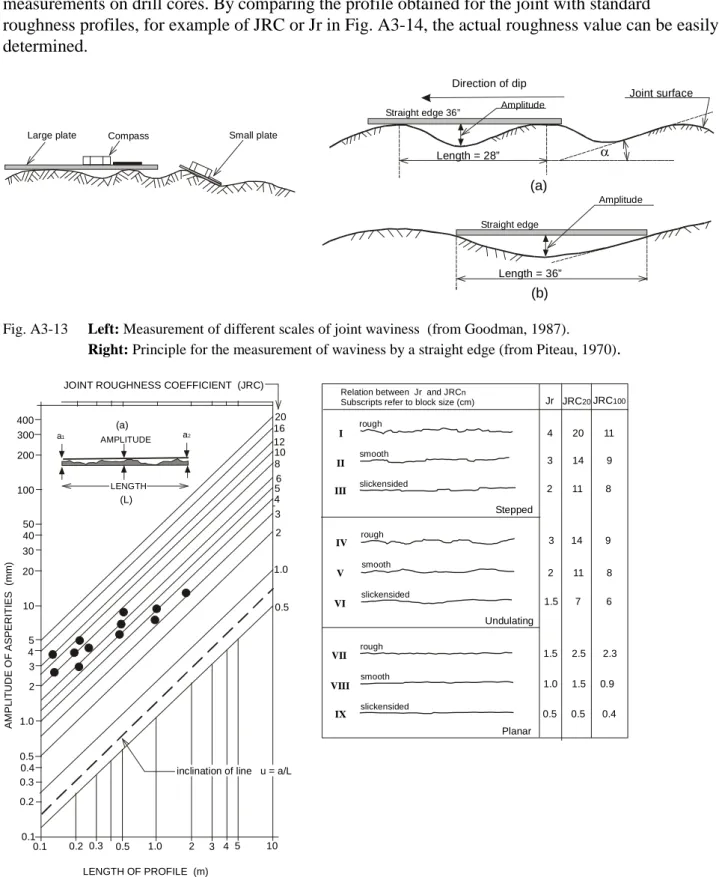
The second is a rapid method, where a few decimetres profile along the joint wall surface is
obtained by a contour gauge and pattern maker. The method is well applicable for joint smoothness measurements on drill cores. By comparing the profile obtained for the joint with standard
roughness profiles, for example of JRC or Jr in Fig. A3-14, the actual roughness value can be easily determined.
Large plate Compass Small plate
Length = 28” Length = 36” Straight edge 36” Direction of dip Joint surface Amplitude Amplitude Straight edge (a) (b) α
Fig. A3-13 Left: Measurement of different scales of joint waviness (from Goodman, 1987).
Right: Principle for the measurement of waviness by a straight edge (from Piteau, 1970).
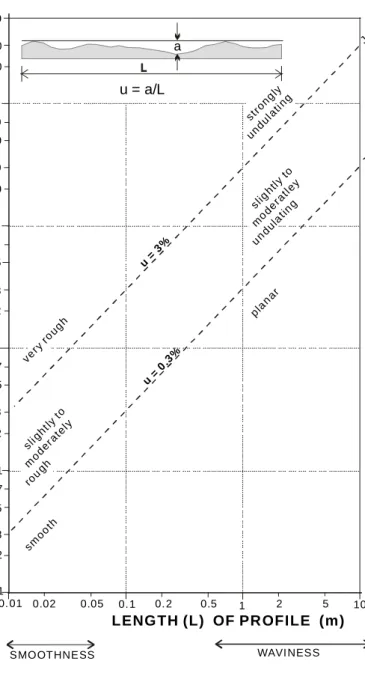
0.1 0.2 0.3 0.5 1.0 2 3 4 5 10 0.1 0.2 0.3 0.4 0.5 1.0 2 3 4 5 10 20 30 40 50 100 200 300 400 AMPLITUDE (a) a1 a2 (L) LENGTH LENGTH OF PROFILE (m) A M P L IT U D E O F A S P E R IT IE S (m m )
JOINT ROUGHNESS COEFFICIENT (JRC)
20 16 12 10 8 6 5 4 3 2 1.0 0.5
inclination of line u = a/L
Relation between Jr and JRC Subscripts refer to block size (cm)
n Jr JRC20JRC100 rough rough rough smooth smooth smooth slickensided slickensided slickensided I II III IV V VI VII VIII IX Stepped Planar Undulating 4 20 11 3 14 9 2 11 8 3 14 9 2 11 8 1.5 7 6 1.5 2.5 2.3 1.0 1.5 0.9 0.5 0.5 0.4
Fig. A3-14 Left: Diagram presented by Barton and Bandis (1992) to estimate JRC for various measuring lengths. The inclined lines exhibit almost a constant undulation as indicated.
Right: Relationships between Jr in the Q-system and the 'joint roughness coefficient' (JRC) for 20 cm and 100 cm sample length (from Barton and Bandis, 1992).
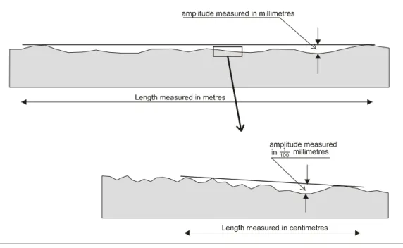
The third technique is generally laborious and, unless the data points are closely spaced along the joint, it does not provide a detailed profile of the small scale roughness. Robertson (1970) and Piteau (1970) have introduced measurement of waviness by using a standard length of 0.9 m (36 inch) straight edge placed on the exposed joint surface in a direction normal to the strike (i.e., down dip).
Amplitude (a) of the wave is a measure of the maximum offset under the straight edge as shown for two different cases in Fig. A3-13 right. This dimension is measured in millimetre. It is related to the length (L), which is recorded as either 1) the distance between adjacent points of contact on the peaks of the wave, Fig. A3-13 right (a), or 2) the standard length adopted, Fig. A3-13 right (b). Also ISRM (1978) has described a similar method to measure the waviness of the joint plane. Kikuchi et al., (1985) has measured waviness of joint plane by selecting portions on a joint plane exposed to the ground, using a 2 m measuring scale. The height of the exposed portions at 2 cm intervals in the direction of dip has been measured to draw the roughness of the joint plane. Also Barton (1982) and Barton and Bandis (1990) make use of a ruler to determine the joint roughness coefficient JRC. Fig. A3-14 shows how different lengths of the ruler can be used to determine JRC. As indicated on this diagram the inclined lines approximately follow the expression for the
undulation factor u = a/L presented later in eq. (A3-12) has been used to find the ratings of the joint waviness factor, jw, where u is applied as shown in Table A3-14.
2.1.2 The joint waviness factor (jw)
As waviness does not change with displacements along the joint surface, no shearing takes place through asperities (Piteau, 1970). The result is that waviness is considered to modify the apparent angle of dip of the joint but not the joint frictional properties. Tsidzi (1986, 1987, 1991) has
observed that waviness is a more characteristic feature of the foliation surface in many metamorphic rocks than the smoothness of the surface.
Waviness of the joint appears as undulations from planarity of the joint wall. Ideally, the joint waviness should be measured as the ratio between max. amplitude over the length of the joint. As it is seldom possible to observe the whole joint plane, a simplified measurement is to find the ratio between max. amplitude and a reduced measured length along the joint plane called the undulation factor
u amplitude from planarity (a) measured length along joint (L)
= eq. (A3-12)
This expression has been used to characterize the waviness of joint plane. From combination of the two diagrams in Fig. A3-14 the division and ratings in Table A3-14 have been worked out. The division here of the undulation is based on the characterization presented by Milne et al. (1992) related to 1 m profile length:
Wavy joints with undulation, u > 2% Planar to wavy joints, with u = 1 - 2% Planar joints, defined as u < 1%.
Their measurements are also based on the 'joint roughness coefficient' (JRC) which is described in Section 2.3.
TABLE A3-14 THE JOINT WAVINESS FACTOR ( jw). THE RATINGS ARE BASED ON Jr IN THE Q-SYSTEM.
TERM FOR WAVINESS waviness factor
undulation jw
Interlocking (large scale) 3
Stepped 2.5
Large undulation u > 3 % 2
Small - moderate undulation u = 0.3 - 3 % 1.5
Planar u < 0.3 % 1
The longest possible ruler should be applied in measurement of waviness. In many cases, however, the determination of (jw) is done from visual observations alone. Practice from ruler measurements may reduce the possible errors in such cases.
0. 1 0. 2 0. 3 0. 5 0. 7 1 2 3 5 7 1 0 20 30 50 70 10 0 20 0 30 0 50 0 0. 01 0.02 0.05 0. 1 0. 2 0.5 1 2 5 10
SMOOTHNESS WAVI NESS
LENG TH (L) OF PR OFILE (m) A M P L IT U D E ( a ) O F A S P E R IT IE S ( m m ) a JC R = 1.5 JC R = 15 u = 0.3 % u = 3% pla nar sm ooth 0. 07 0. 05 0. 03 0. 02 0. 01 u = a/L s tron gly undu lati ng slig htly to m ode ratl ey und ula ting very rou gh slig htly to m ode rate ly rou gh
2.1.3 The joint smoothness factor (js)
Small asperities or second order projections are designated smoothness or unevenness. If the joint surfaces are clean and closed these small asperities interlock to strongly contribute to the shear resistance especially at low stresses (Barton and Chubey, 1977; Barton, 1976, 1987, 1990b, 1993). Smoothness asperities usually have a base length of some centimetres and amplitude measured in hundreds of millimetres and are readily apparent on a core-sized exposure of a discontinuity (see Fig. A3-12 and A3-15).
As indicated in Fig. A3-12 and A3-15 the 'sample length' for smoothness is in the range of a few centimetres. There is a general problem to arrive at a numerical estimate of joint smoothness from measurements or visual observations of the joint wall surface. A possible solution is to simply touch the surface with the finger and compare it with a reference surface of known roughness, for example sand papers of various abrasivity (mesh) as indicated in Table A3-16.
The terms and ratings defined in Table A3-16 are based on Jr in the Q-system (Barton et al., 1974), while the description is also partly based on Bieniawski (1984).
TABLE A3-16 THE JOINT SMOOTHNESS FACTOR (js). THE RATINGS ARE THE SAME AS FOR Jr IN THE Q-SYSTEM. (The description is partly based on Bieniawski, 1984).
TERM FOR SMOOTHNESS DESCRIPTION The smoothness factor js Very rough Rough Slightly rough Smooth Polished Slickensided
Near vertical steps and ridges occur with interlocking effect on the joint surface.
Some ridge and side-angle steps are evident; asperities are clearly visible; discontinuity surface feels very abrasive (rougher than sandpaper grade 30)
Asperities on the discontinuity surfaces are distinguishable and can be felt (like sandpaper grade 30 - 300).
Surface appear smooth and feels so to the touch (smoother than sandpaper grade 300).
Visual evidence of polishing exists. This is often seen in coatings of chlorite and specially talc
Polished and striated surface that results from friction along a fault surface or other movement surface.
3 2 1.5 1 0.75 0.6 - 1.5 1) 1)
Rating depends on the actual shear in relation to the striations.
2.1.4 The joint roughness factor (jR) found from jw and js
As described in the foregoing the smoothness and waviness can both be characterized by the ratio between the amplitude of asperities and the measuring length as shown in Fig. A3-15. A similar principle has been presented by Milne et al. (1992) who have used the joint roughness coefficient (JRC) to also assess small scale roughness (i.e. smoothness) using 10 cm profile lengths with the following division:
- rough surfaces JRC > 10 (undulation u > 2%)
The joint roughness factor, jR, is the product of the smoothness and waviness factors:
jR = js × jw eq. (A3-13)
which is shown in Table A3-17.
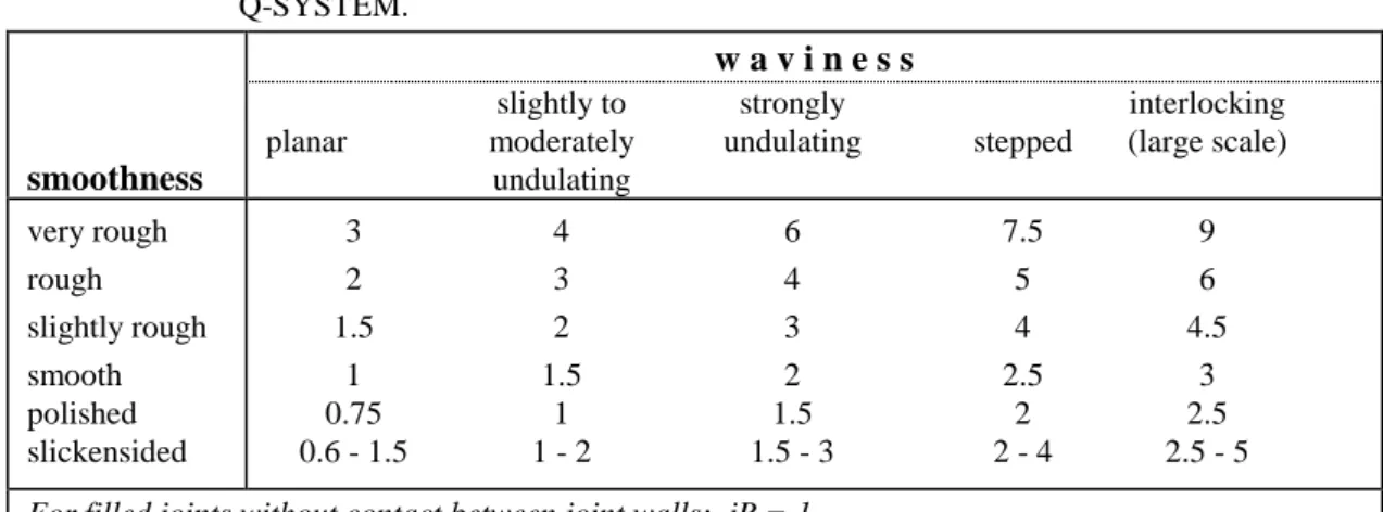
TABLE A3-17 JOINT ROUGHNESS FACTOR (jR) FROM SMOOTHNESS AND WAVINESS. THE STRUCTURE OF THE FACTOR AND ITS RATING ARE SIMILAR TO Jr IN THE Q-SYSTEM.
smoothness
w a v i n e s s
slightly to strongly interlocking
planar moderately undulating stepped (large scale) undulating very rough rough slightly rough smooth polished slickensided 3 4 6 7.5 9 2 3 4 5 6 1.5 2 3 4 4.5 1 1.5 2 2.5 3 0.75 1 1.5 2 2.5 0.6 - 1.5 1 - 2 1.5 - 3 2 - 4 2.5 - 5
For filled joints without contact between joint walls: jR = 1
Joint roughness includes the condition of the joint wall surface both for filled and unfilled (clean) joints. For joints with filling which is thick enough to avoid contact of the two joint walls, any shear movement will be restricted to the filling, and as described later, the joint roughness will then have minor or no importance. In the cases of filled joints it is often difficult or impossible to measure the smoothness and often also the waviness. Therefore the roughness factor is defined as jR = 1 as in the Q system.
The joint roughness coefficient, jR (or Jr) can also be found from measured values of JRC using Fig. A3-14 or A3-15.
The classification systems which often make use of many a large amount of input data, the ratings for roughness are mostly found from observations. It is, therefore, not common to make detailed measurements of joint roughness profiles.
2.2 Estimating the joint alteration factor (jA)
"It is often more important to characterize discontinuities according to surface character as it is to note their scale parameters."
Tor L. Brekke and Terry R. Howard (1972)
The joint alteration factor is a collective parameter including the strength of the joint wall and the possible joint filling, whether it is a clean or a filled joint. The following features are included in this complex factor:
− The condition of the surface in clean joints, i. e. joints without coating or filling; with indication if alteration of the joint wall may be other than the rock.
− The type of coating on the joint surface.
2.2.1 Clean joints
Clean joints are without fillings or coatings. For these joints the compressive strength of the rock wall is a very important component of shear strength and deformability where the walls are in direct rock to rock contact (ISRM, 1978).
Close to the surface in outcrops it is imperative not to confuse clean discontinuities with "empty" discontinuities where filling material has been leached and washed away due to surface weathering. Clean joints can be:
a. Healed or welded joints. Joints, seams and sometimes even minor faults may be healed through precipitation from solutions of quartz, epidote or calcite. In such cases the joint plane can be regarded more appropriately as a plane of reduced strength.
b. Healed joints may, however, have broken up again, forming new surfaces. Also, it should be emphasized that quartz and calcite may well be present in a discontinuity without healing it. c. Fresh rock walls. These are joint walls of unweathered or unaltered rock. They may, however,
show staining (rust) on the surfaces.
d. Altered or weathered rock walls. Some clean joints may show alteration of the rock material on the joint surface (Piteau, 1970). The rock surface in these joints can be in the same condition as the rock elsewhere. Often, however, when weathering or alteration has taken place it is more pronounced along the joint surface than in the rock. This results in a wall strength often considerably lower than that of the fresher rock found in the interior of the rock blocks. The degree of weathering is usually estimated from visual observations. It can partly be quantified applying the ISRM classification of alteration and weathering (see Table A3-12), and should be applied in jA where it differs from the alteration of the rock material, as is shown in Table A3-21.
2.2.2 Coated joints
Coating means that the joint surfaces have a thin layer or 'paint' with some kind of mineral. The coating, which is not thicker than a few millimetres, can consist of various kinds of mineral matter, such as chlorite, calcite, epidote, clay, graphite, zeolite. Mineral coatings will affect the shear strength of joints to a marked degree if the surfaces are planar. The properties of the coating
material may dominate the shear strength of the joint surface, especially weak and slippery coatings of chlorite, talc and graphite when wet.
2.2.3 Filled joints
Filling or gouge when used in general terms, is meant to include any material different from the rock thicker than coating which occurs between two discontinuity planes. Thickness of the filling or gouge is taken as the width of that material between sound intact rock. Table A3-18 shows the classification of joint or seam thickness presented by ISRM (1978).
Unless discontinuities are exceptionally smooth and planar, it will not be of great significance to the shear strength that a 'closed' feature is 0.1 mm wide or 1.0 mm wide, ISRM (1978). (However, indirectly as a result of hydraulic conductivity, even the finest joints may be significant in changing the normal stress and therefore also the shear strength.)
TABLE A3-18 SEPARATION OF DISCONTINUITY WALLS (from Bieniawski 1984) Very tight < 0.1 mm Tight 0.1 - 0.5 mm Moderately open 0.5 - 2.5 mm Open 2.5 - 10 mm Very open 10 - 25 mm
Aperture is the perpendicular distance separating the adjacent rock walls of an open discontinuity, in which the intervening space is air or water filled. Aperture is thereby distinguished from the width of a filled discontinuity (ISRM, 1978).)
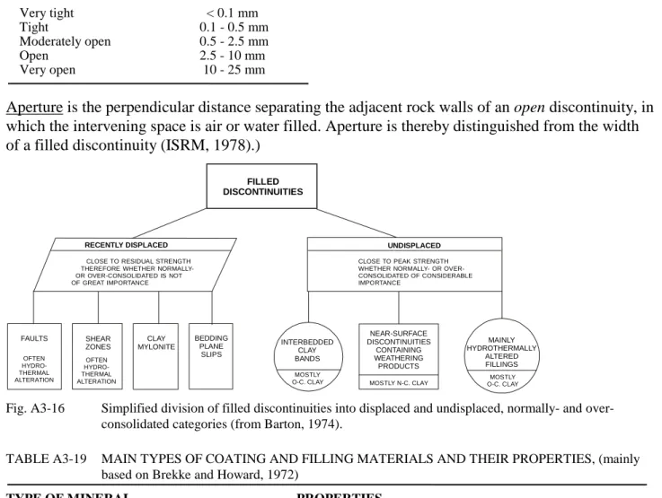
RECENTLY DISPLACED FILLED DISCONTINUITIES UNDISPLACED FAULTS SHEAR ZONES CLAY MYLONITE BEDDING PLANE SLIPS INTERBEDDED CLAY BANDS NEAR-SURFACE DISCONTINUITIES CONTAINING WEATHERING PRODUCTS MAINLY HYDROTHERMALLY ALTERED FILLINGS OFTEN HYDRO-THERMAL ALTERATION OFTEN HYDRO-THERMAL ALTERATION MOSTLY
O-C. CLAY MOSTLY N-C. CLAY O-C. CLAYMOSTLY
CLOSE TO RESIDUAL STRENGTH THEREFORE WHETHER OR OVER-CONSOLIDATED IS NOT OF GREAT IMPORTANCE
CLOSE TO PEAK STRENGTH WHETHER NORMALLY- OR OVER-CONSOLIDATED OF CONSIDERABLE IMPORTANCE
Fig. A3-16 Simplified division of filled discontinuities into displaced and undisplaced, normally- and over-consolidated categories (from Barton, 1974).
TABLE A3-