Database Plan Quality Impact on Knowledge-based Radiation Therapy Treatment Planning of Prostate Cancer

(1)

Louisiana State University

LSU Digital Commons

LSU Master's Theses Graduate School

2017

Database Plan Quality Impact on

Knowledge-based Radiation Therapy Treatment Planning of

Prostate Cancer

Phillip Douglas Hardenbergh Wall

Louisiana State University and Agricultural and Mechanical College, [email protected]

Follow this and additional works at:https://digitalcommons.lsu.edu/gradschool_theses

Part of thePhysical Sciences and Mathematics Commons

This Thesis is brought to you for free and open access by the Graduate School at LSU Digital Commons. It has been accepted for inclusion in LSU Master's Theses by an authorized graduate school editor of LSU Digital Commons. For more information, please [email protected]. Recommended Citation

Wall, Phillip Douglas Hardenbergh, "Database Plan Quality Impact on Knowledge-based Radiation Therapy Treatment Planning of Prostate Cancer" (2017).LSU Master's Theses. 4443.

(2)

DATABASE PLAN QUALITY IMPACT ON KNOWLEDGE-BASED

RADIATION THERAPY TREATMENT PLANNING OF PROSTATE CANCER

A Thesis

Submitted to the Graduate Faculty of the Louisiana State University and Agricultural and Mechanical College

in partial fulfillment of the requirements for the degree of

Master of Science in

The Department of Physics and Astronomy

by

Phillip Douglas Hardenbergh Wall B.S., Davidson College, 2014

(3)

ACKNOWLEDGEMENTS

My deepest gratitude goes to my major advisor, Dr. Jonas Fontenot, for the opportunity to work with him on this project. I have learned so much from him and I thank him for his helpful guidance and support over the course of this research. I also thank Dr. Robert Carver for his valuable contributions and insight, especially in our discussions of the more technical aspects of the project. I also thank committee members, Drs. Rui Zhang and Juhan Frank, for investing their time and expertise in supervising and monitoring this project.

I want to acknowledge all faculty and staff involved with the medical physics program at Louisiana State University (LSU) and Mary Bird Perkins Cancer Center. I appreciate the professors and thank them for helping me through my studies, particularly Dr. Kenneth Matthews for his incredible commitment to helping all program students. I want to especially thank David Perrin and Connel Chu for helping me with compiling the patient database for this project. I also express my sincerest thanks and appreciation for administrators Susan Hammond, Megan Jarrell, Katherine Pevey, and LaShawn Burns for helping with logistics and paperwork throughout my LSU career.

Additional thanks go to Jie Chen and Dr. David Blouin of the LSU Department of

Experimental Statistics for their assistance in forming the statistical design and methods used in this project. Also, I thank Cameron Ditty, Senior Physics Specialist for RaySearch Laboratories, for assisting me with the nuances of scripting in RayStation, which allowed me to develop the scripts needed for this project.

I also want to thank all my student colleagues I have known in my time at LSU for their camaraderie. I specifically acknowledge my fellow classmates John Doiron, Krystal Kirby, and Xiaodong Zhao for helping me navigate through graduate studies.

Finally, I thank my mother, brother, and grandfather for their unwavering love and support, which have always been and will always be my biggest motivator and inspiration.

(4)

LIST OF TABLES

Table 1: Distribution of patient characteristics in the database. The selected patients cover a wide range of prescription doses, treatment areas, and target volumes. SV stands for seminal vesicle involvement and LN stands for lymph node involvement. ... 17 Table 2: MCO planning objectives and constraints used in generating balance plans for each

database patient. The Dose Fall-off objective for the External structure reduces dose outside of the target. Rx refers to the prescription dose. ... 18 Table 3: Pearson correlation coefficients between nominal OVH distances and DVH dose-volumes

of the bladder and rectum. An absolute value greater than 0.7 indicates a strong linear correlation with a maximum value of 1. ... 20 Table 4: Pearson correlation coefficients between each second-order factor and DVH dose-volumes for the bladder and rectum. The mean Pearson coefficient over the four fractional volumes is also listed. Only the in-field OAR volume was strongly correlated (mean greater than 0.7) for both the bladder and rectum. ... 24 Table 5: Pearson correlation coefficients between in-field OVH distances and DVH dose-volumes

of the bladder and rectum. The correlation coefficients between the nominal OVH distances and DVH dose-volumes from Table 3 are also listed for comparison. Note that n refers to the number of database patients with in-field OAR volumes greater than or equal to the given dose-volume. ... 25 Table 6: Dose metrics used to statistically verify clinical PTV and secondary OAR dose was

maintained in the re-plans. Vx represents the percent volume receiving x% of the

prescription dose. ... 35 Table 7: Statistical comparison of CPD and MCOD KBP model and clinical dose-volumes, with

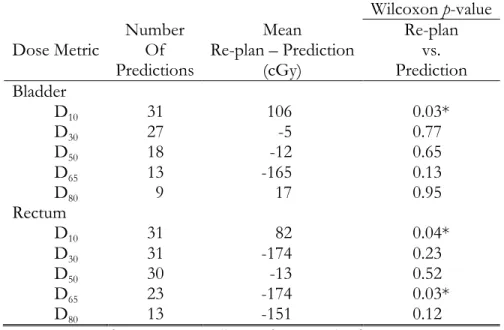
associated mean differences between combinations of the clinical, CPD model, and MCOD model dose values. These mean differences correspond to the grey circles in Figure 9. ... 39 Table 8: Statistical results of the dose comparison between the clinical plans and re-plans for the

PTV and secondary OARs. While the PTV and femoral head dose metrics were averaged over the 31 patients, the penile bulb was averaged over the 28 patients in which it was segmented. ... 41 Table 9: Average differences in re-planned and clinical dose values over the 31 patients with

Wilcoxon test results for the primary OARs. ... 43 Table 10: Dosimetric and statistical results for evaluating prediction performance and achievability.

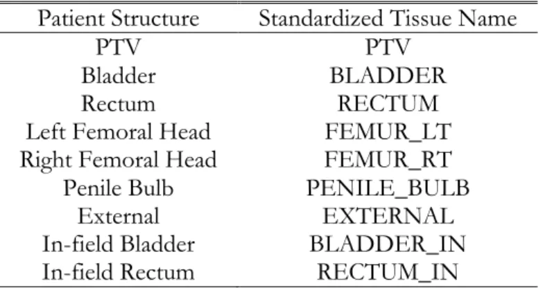
... 44 Table 11: List of structures used in this study and their assigned standardized Tissue Name labels.

The in-field structures were created for computing the in-field OVH in this study as will be discussed in A.3. ... 61

(7)

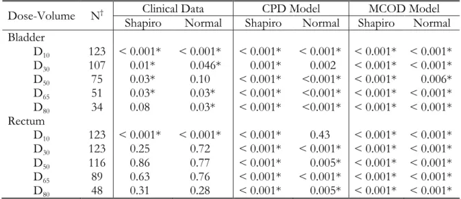
Table 12: Normality statistical test p-values for the three distributions of data. A statistically significant result may be interpreted as the given data likely representing a non-normal distribution. ... 65 Table 13: Results from the omnibus test. Each dose-volume yielded statistically significant results,

indicating a difference likely exists between the three distributions of data. ... 67 Table 14: Summary of the Pearson correlation coefficients for the distance-to-dose relationships

formed with the CPD and MCOD dose data. The nominal OVH data was used for these correlations. The MCOD dose produced a stronger correlation with distance overall, most noticeably in the rectum. This is most likely due to the removal of the inter-planner

subjectivity present in the CPD dose data. ... 72 Table 15: Statistical results of the dose comparison between the two plan databases for the PTV and

secondary OARs. The mean differences between the MCOD and CPD dose metrics were averaged over the 124 database patients. ... 97 Table 16: Statistical results of the dose comparison between the two plan databases for the primary

OARs. The mean differences between the MCOD and CPD dose metrics were averaged over the 124 database patients. ... 98 Table 17: Statistical results comparing predictions from KBP model using the in-field OVH versus

(8)

LIST OF FIGURES

Figure 1: Diagram of a modern linear accelerator, highlighting the three varying parameters that differentiate VMAT from other EBRT delivery techniques.13,14_{... 3}

Figure 2: An example from RaySearch Laboratories of a three-dimensional Pareto surface for a prostate plan with three MCO trade-off objectives. The planner can search over this surface in real-time to consider different clinical trade-offs.24_{... 7}

Figure 3: Example of dose distribution differences between inverse and MCO planning. The same axial CT slice of the same prostate patient is shown with the inversely optimized clinical VMAT plan on top (a) and a deliverable balance MCO VMAT plan on bottom (b). A noticeable reduction in OAR dose is shown in the MCO plan, particularly for both femoral heads. ... 8 Figure 4: Illustration from Wu et al. relating the distance a fractional OAR volume (v) lies from the

PTV surface (rv) on the OVH (left) to the dose the fractional volume receives (Dv) on the DVH (right).63_{... 13}

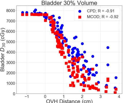
Figure 5: Nominal DVH-OVH correlations for 30, 50, 65, and 80% dose-volumes of the bladder (a, c, e, g) and rectum (b, d, f, h). ... 21 Figure 6: Sample color scatter plots for qualitative review of dependence on the examined

second-order factors. There is no visible relationship between dose and PTV volume for neither 65% of the bladder (a) nor the rectum (b). When analyzing in-field OAR volume however, a clear relationship with D65 for the bladder (c) and rectum (d) can be seen. ... 23

Figure 7: Representative examples of improved distance-to-dose correlations using the in-field OVH compared with the nominal OVH. The figure legends contain the number of patients (n) and the Pearson correlation coefficients (R) for each OVH method. The square nominal OVH data points are equivalent to the scatter plots shown in Figure 5. ... 26 Figure 8: Comparison between the average DVHs of the labeled planning structures from plans in

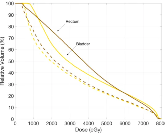
the CPD (solid lines) and MCOD (dashed lines). Note: the femoral heads are plotted separately (i.e. left and right femoral heads) but are difficult to resolve as they are nearly identical and their curves overlap each other. ... 36 Figure 9: Set of boxplots showing differences in dose-volumes between the clinical plan values, the

CPD KBP model predictions, and MCOD KBP model predictions for the bladder (a) and the rectum (b). Below each dose-volume lists the number of patients, n, where a KBP prediction was possible under the protocol detailed in Chapter 3.1.3. Note: data points outside boxplot whiskers are more than 1.5 times the interquartile range (first quartile to third quartile i.e. length of boxes) from the first or third quartiles, the grey circles represent the mean of each distribution, and the horizontal black lines within each box represent the median of each distribution. ... 37

(9)

Figure 10: Average PTV and secondary OAR DVHs of the 31 re-planned patients comparing the clinical plans (solid lines) and re-plans (dashed lines). Note the penile bulb was not

segmented in 3 of the 31 patients. ... 40 Figure 11: Average DVHs over the 31 patients of the bladder and rectum for the clinical plans (solid lines) and re-plans (dashed lines). ... 42 Figure 12: Sagittal CT slice of a database patient showing the estimation of the treatment fields. The horizontal lines are part of the ROI created from the original PTV contour to represent the treatment fields. Given Tissue Names are listed with their corresponding ROIs, with the in-field OAR portions indicated by “_IN.” Note the femoral heads are not visible and are located to the left and right of the shown CT slice. ... 63 Figure 13: Representative examples of data visualization via density distribution histograms along

with estimated normal curves, plotted using the mean and standard deviation of the data. (a) is an example of a distribution determined to likely be non-normal and (b) is an example of a distribution deemed to be normal. ... 66 Figure 14: Nominal DVH-OVH correlation (R) using the CPD DVH data (circles) and the MCOD

DVH data (squares) for the 30% dose-volume of the bladder. ... 68 Figure 15: Nominal DVH-OVH correlation (R) using the CPD DVH data (circles) and the MCOD

DVH data (squares) for the 30% dose-volume of the rectum. ... 70 Figure 19: Nominal DVH-OVH correlation (R) using the CPD DVH data (circles) and the MCOD

DVH data (squares) for the 80% dose-volume of the rectum. ... 71 Figure 22: Color bar scatter plot for distance-to-dose relationship for 30% of the bladder, where the color-mapped variable is the derivative of the OVH. ... 73 Figure 23: Color bar scatter plot for distance-to-dose relationship for 50% of the bladder, where the color-mapped variable is the derivative of the OVH. ... 73

(10)

Figure 24: Color bar scatter plot for distance-to-dose relationship for 65% of the bladder, where the color-mapped variable is the derivative of the OVH. ... 74 Figure 25: Color bar scatter plot for distance-to-dose relationship for 80% of the bladder, where the color-mapped variable is the derivative of the OVH. ... 74 Figure 26: Color bar scatter plot for distance-to-dose relationship for 30% of the rectum, where the

color-mapped variable is the derivative of the OVH. ... 75 Figure 27: Color bar scatter plot for distance-to-dose relationship for 50% of the rectum, where the

color-mapped variable is the derivative of the OVH. ... 76 Figure 30: Color bar scatter plot for distance-to-dose relationship for 30% of the bladder, where the color-mapped variable is the prescription dose. ... 77 Figure 31: Color bar scatter plot for distance-to-dose relationship for 50% of the bladder, where the color-mapped variable is the prescription dose. ... 77 Figure 32: Color bar scatter plot for distance-to-dose relationship for 65% of the bladder, where the color-mapped variable is the prescription dose. ... 78 Figure 33: Color bar scatter plot for distance-to-dose relationship for 80% of the bladder, where the color-mapped variable is the prescription dose. ... 78 Figure 34: Color bar scatter plot for distance-to-dose relationship for 30% of the rectum, where the

color-mapped variable is the prescription dose. ... 79 Figure 35: Color bar scatter plot for distance-to-dose relationship for 50% of the rectum, where the

color-mapped variable is the prescription dose. ... 80 Figure 38: Color bar scatter plot for distance-to-dose relationship for 30% of the bladder, where the color-mapped variable is the PTV volume. ... 81 Figure 39: Color bar scatter plot for distance-to-dose relationship for 50% of the bladder, where the color-mapped variable is the PTV volume. ... 81

(11)

Figure 40: Color bar scatter plot for distance-to-dose relationship for 80% of the bladder, where the color-mapped variable is the PTV volume. ... 82 Figure 41: Color bar scatter plot for distance-to-dose relationship for 30% of the rectum, where the

color-mapped variable is the PTV volume. ... 82 Figure 42: Color bar scatter plot for distance-to-dose relationship for 50% of the rectum, where the

color-mapped variable is the PTV volume. ... 83 Figure 43: Color bar scatter plot for distance-to-dose relationship for 80% of the rectum, where the

color-mapped variable is the PTV volume. ... 83 Figure 44: Color bar scatter plot for distance-to-dose relationship for 30% of the bladder, where the color-mapped variable is the bladder volume. ... 84 Figure 45: Color bar scatter plot for distance-to-dose relationship for 50% of the bladder, where the color-mapped variable is the bladder volume. ... 84 Figure 46: Color bar scatter plot for distance-to-dose relationship for 65% of the bladder, where the color-mapped variable is the bladder volume. ... 85 Figure 47: Color bar scatter plot for distance-to-dose relationship for 80% of the bladder, where the color-mapped variable is the bladder volume. ... 85 Figure 48: Color bar scatter plot for distance-to-dose relationship for 30% of the rectum, where the

color-mapped variable is the bladder volume. ... 86 Figure 49: Color bar scatter plot for distance-to-dose relationship for 50% of the rectum, where the

color-mapped variable is the bladder volume. ... 87 Figure 52: Color bar scatter plot for distance-to-dose relationship for 30% of the bladder, where the color-mapped variable is the rectum volume. ... 88 Figure 53: Color bar scatter plot for distance-to-dose relationship for 50% of the bladder, where the color-mapped variable is the rectum volume. ... 88 Figure 54: Color bar scatter plot for distance-to-dose relationship for 65% of the bladder, where the color-mapped variable is the rectum volume. ... 89 Figure 55: Color bar scatter plot for distance-to-dose relationship for 80% of the bladder, where the color-mapped variable is the rectum volume. ... 89

(12)

Figure 56: Color bar scatter plot for distance-to-dose relationship for 30% of the rectum, where the color-mapped variable is the rectum volume. ... 90 Figure 57: Color bar scatter plot for distance-to-dose relationship for 50% of the rectum, where the

color-mapped variable is the rectum volume. ... 90 Figure 58: Color bar scatter plot for distance-to-dose relationship for 65% of the rectum, where the

color-mapped variable is the rectum volume. ... 91 Figure 59: Color bar scatter plot for distance-to-dose relationship for 80% of the rectum, where the

color-mapped variable is the rectum volume. ... 91 Figure 60: Color bar scatter plot for distance-to-dose relationship for 30% of the bladder, where the color-mapped variable is the in-field OAR volume. ... 92 Figure 61: Color bar scatter plot for distance-to-dose relationship for 50% of the bladder, where the color-mapped variable is the in-field OAR volume. ... 92 Figure 62: Color bar scatter plot for distance-to-dose relationship for 80% of the bladder, where the color-mapped variable is the in-field OAR volume. ... 93 Figure 63: Color bar scatter plot for distance-to-dose relationship for 30% of the rectum, where the

color-mapped variable is the in-field OAR volume. ... 93 Figure 64: Color bar scatter plot for distance-to-dose relationship for 50% of the rectum, where the

color-mapped variable is the in-field OAR volume. ... 94 Figure 65: Color bar scatter plot for distance-to-dose relationship for 80% of the rectum, where the

color-mapped variable is the in-field OAR volume. ... 94 Figure 66: DVH-OVH correlation (R) using nominal OVH data (squares) and in-field OVH data

(diamonds) for the 30% dose-volume of the bladder. ... 95 Figure 67: DVH-OVH correlation (R) using nominal OVH data (squares) and in-field OVH data

(diamonds) for the 50% dose-volume of the bladder. ... 95 Figure 68: DVH-OVH correlation (R) using nominal OVH data (squares) and in-field OVH data

(diamonds) for the 30% dose-volume of the rectum. ... 96 Figure 69: DVH-OVH correlation (R) using nominal OVH data (squares) and in-field OVH data

(diamonds) for the 50% dose-volume of the rectum. ... 96 Figure 70: Patient-by-patient data from re-planning study comparing the original, clinical value

(triangle), in-field OVH KBP prediction (square), standard OVH KBP prediction (diamond), and re-planned value (circle) for bladder D10. ... 99

Figure 71: Patient-by-patient data from re-planning study comparing the original, clinical value (triangle), in-field OVH KBP prediction (square), standard OVH KBP prediction (diamond), and re-planned value (circle) for bladder D30. ... 99

(13)

Figure 75: Patient-by-patient data from re-planning study comparing the original, clinical value (triangle), in-field OVH KBP prediction (square), standard OVH KBP prediction (diamond), and re-planned value (circle) for rectum D10. ... 101

(14)

ABSTRACT

Purpose: Knowledge-based planning (KBP) leverages plan data from a database of previously treated patients to inform the plan design of a new patient. This work investigated bladder and rectum dose-volume prediction improvements in a common KBP method using a Pareto plan database in VMAT planning for prostate cancer.

Methods: We formed an anonymized retrospective patient database of 124 VMAT plans for prostate cancer treated at our institution. From these patient data, two plan databases were compiled. The clinical plan database (CPD) contained planning data from each patient’s clinical plan, which were manually optimized by various planners. The multi-criteria optimization database (MCOD)

contained Pareto plan data from plans created using a standardized MCO protocol. Overlap volume histograms, incorporating fractional OAR volumes only within the treatment fields, were computed for each patient and used to match new patient anatomy to similar database patients. For each database patient, CPD and MCOD KBP predictions were generated for D10, D30, D50, D65, and D80

of the bladder and rectum in a leave-one-out manner. Prediction achievability was verified through a re-planning study on a subset of 31 randomly selected database patients using the lowest KBP predictions, regardless of plan database origin, as planning goals.

Results: MCOD model predictions were significantly lower (p < 0.001) than CPD model predictions for all five bladder dose-volumes and rectum D50 (p = 0.004) and D65 (p < 0.001), while CPD model

predictions for rectum D10 (p = 0.005) and D30 (p < 0.001) were significantly less than MCOD model

predictions. KBP model predictions were statistically equivalent to re-planned values for all predicted dose-volumes, excluding D10 of bladder (p = 0.03) and rectum (p = 0.04). Compared to

clinical plans, re-plans showed significant average reductions in Dmean for bladder (7.8 Gy; p < 0.001)

and rectum (9.4 Gy; p < 0.001), while maintaining statistically similar PTV, femoral head, and penile bulb dose.

(15)

Conclusion: KBP dose-volume predictions derived from Pareto plans were lower overall than those resulting from manually optimized clinical plans. A re-planning study showed the KBP dose-volume predictions were achievable and led to significant reductions in bladder and rectum dose.

(16)

CHAPTER 1. INTRODUCTION

1.1 BACKGROUND

1.1.1 RADIATION THERAPY TREATMENT DELIVERY AND PLANNING

Radiation therapy (or radiotherapy) is the use of high-energy radiation, such as x-rays, gamma rays, electrons, or protons, to kill or damage cancer cells. Over half of all cancer patients will receive some form of radiotherapy during the course of their treatment.1_{Currently, there are two}

main approaches to delivering the prescribed radiation dose: external beam radiotherapy (EBRT), which involves large source-to-surface distances, or SSDs; and brachytherapy, which utilizes radioisotopes to treat internally or with small SSDs. In EBRT, linear accelerators are used to generate and direct megavoltage electrons or photons toward the cancer located within the patient.

Most modern linear accelerators support different options for delivering the prescribed radiation dose to the target for a given patient and disease. 3D conformal radiotherapy (3DCRT) collimates radiation fields of uniform intensity around lesions to simultaneously dose the target and spare surrounding healthy tissues using multi-leaf collimators (MLCs), which are motorized sets of thin, tungsten slabs that move in and out of the field to form different shapes.2_{3DCRT was the first}

delivery technique based on 3D anatomical information provided by computed tomography (CT) scans. Access to 3D information allows more accurate delineations of targets and healthy organs and conformal dose distributions compared to previous delivery methods based on 2D radiographic projections.

Alternatively, fixed-field intensity modulated radiotherapy (IMRT) is a delivery technique typically combining five to seven fixed radiation fields of spatially varying fluence patterns. Each beam’s modulated intensity profiles are achieved by combining complex sequences of MLC leaf travel, which are set to optimize the composite dose distribution. IMRT combines the non-uniform fluence maps from each beam (aimed from different directions) to create highly conformal dose

(17)

distributions that improve target coverage and in sparing of normal tissues compared to 3DCRT.3,4

However, longer treatment delivery times and increased monitor units (MUs) are limitations for IMRT treatments. The latter can increase radiation exposure to parts of the body distant from the treatment field, whereas the former can impair patient comfort and reproducibility.5_{In order to}

overcome these deficiencies, arc-based or rotational treatment techniques were developed, where radiation is delivered while rotating the linear accelerator about the target.

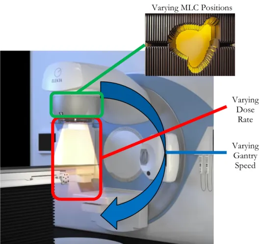
Volumetric modulated arc therapy (VMAT), one such rotational IMRT technique, delivers intensity modulated fields by continuously varying three main parameters: rotation speed of the linear accelerator gantry, MLC positions, and dose rate (Figure 1).6_{VMAT dose is computed by}

approximating a continuous arc with a large number of discrete segments. The non-uniform fluence profiles and ensuing MLC sequences are optimized at each control point (each segment lies between two control points) to create highly conformal intensity modulated dose distributions. Compared to fixed-field IMRT, VMAT requires fewer MUs and provides a significantly shorter treatment time.7

Due to the relatively recent clinical implementation of VMAT, its overall dosimetric advantages over fixed-field IMRT are uncertain. Some studies have reported potential benefits of VMAT for specific treatment sites like the prostate, while others have found inconsistent dosimetric results between IMRT and VMAT for head-and-neck treatments.7-12_{Primarily owing to efficiency, VMAT has}

quickly become a ubiquitous treatment technique for cases requiring intensity modulation.

Radiotherapy treatment planning is the process of defining how the prescribed dose is to be delivered during treatment. More specifically, a treatment plan specifies the machine parameters to produce the desired dose distribution for the given patient. These parameters can include the number of beams, beam energy, beam shape, beam weight, gantry angle, intensity modulators (e.g. wedges, tissue compensators, MLCs), and couch angle. Computerized treatment planning systems (TPSs) are used to help determine these parameters to arrive at a customized treatment plan for each

(18)

patient. Even with the assistance of computers, treatment plan design is time-consuming and highly complex given the large number of parameters the must be specified.

Figure 1: Diagram of a modern linear accelerator, highlighting the three varying parameters that differentiate VMAT from other EBRT delivery techniques.13,14

There are two main approaches to treatment planning used today, each of which facilitate specific delivery techniques. “Forward planning” is employed to design treatment plans for conventional, uniform intensity techniques (e.g. 3DCRT). Forward planning is the process of manually adjusting treatment parameters to obtain the desired dose distribution. If a patient is to be treated with 3DCRT, for instance, the planners must manually find the appropriate machine and treatment parameters to obtain an acceptable plan. This forward planning approach forces planners to determine these parameters effectively by trial-and-error, where the dose must be computed and evaluated each time a set of parameters is selected. Moreover, if the resulting dose distribution is not

Varying MLC Positions Varying Dose Rate Varying Gantry Speed

(19)

acceptable, the parameters are manually adjusted and the dose is recomputed for evaluation. These iterations continue until the desired dose distribution is achieved.

Alternatively, “inverse planning” is used for planning more complex treatment delivery techniques such as IMRT and VMAT. These techniques require many intricate MLC sequences for each field or arc segment to generate the necessary modulated fluence patterns. Manually optimizing these varying fluence maps and corresponding MLC sequences for each beam via forward planning would prove prohibitively difficult and laborious.15_{Therefore, inverse planning optimization}

algorithms were developed and implemented into TPSs to plan these intensity modulated delivery techniques. Inverse planning requires the planner to specify the clinical treatment criteria, after which an optimization algorithm automatically determines modulated fluence maps for each beam or arc segment that achieve the treatment goals. More specifically, the user defines clinical dose-volume constraints (i.e. the dose a fractional dose-volume of a planning structure receives) for the target and normal tissues, which are represented as cost objective functions for the optimization algorithm to minimize. Once the optimizer generates a set of modulated fluence segments and beam

parameters for the given treatment objectives, the dose is computed and the dose distribution is evaluated. If improvement is needed or the planner wants to assess a clinical trade-off, the planner must adjust the initial dose-volume objectives and run another optimization. Additionally, clinical inverse planning algorithms utilize a gradient-based search for optimal intensity profiles, which usually requires multiple optimization rounds to ensure the solution reaches a global, and not a local, minimum. This trial-and-error nature of inverse planning resembles that of forward planning, but the two protocols differ in the parameters that planners modify after each iteration. Regardless, inverse planning can become increasingly time-consuming for complicated cases, like head-and-neck patients, that require the assessment of a large number of clinical trade-offs. Paired with the time limitations of a clinical environment, this can limit the quality of inverse plans.

(20)

While it drives the planning of IMRT techniques, inverse optimization reduces a three-dimensional dose distribution into a set of dose objectives based on one-three-dimensional dose volume histograms (DVHs). This dimensionality reduction in describing dose distributions underscores the importance of selecting and adjusting optimal inverse planning objectives. Planners do not currently know a priori what the fully optimal treatment plan is for a given patient, let alone the set of planning objectives needed to arrive at that plan. Further, clinical dose-volume goals for normal tissues are usually derived from population-based clinical studies (e.g. Emami et al.16_{, Quantitative Analysis of}

Normal Tissue Effects in the Clinic17_{, Radiation Therapy Oncology Group studies, etc.), which have}

recommended dose tolerances for clinical acceptability but do not provide any patient-specific information. This, in addition to unique patient anatomies and the heuristic nature of inverse planning, cause the quality of inversely optimized plans to be susceptible to planner bias and subjectivity. These limitations of inverse planning have led studies to observe a plan quality dependence on planner experience and “skill.”18_Batumalai_{et al}_{. found within one institution that}

more experienced planners were able to produce superior IMRT plans for a head-and-neck case compared with less experienced planners, whose plans were also generally more difficult to deliver accurately.19_{Planner bias results in plan quality variations between planners and institutions, which}

lead to sub-optimal plans that are clinically-acceptable but more sparing of organs at risk (OARs) is possible.20,21_Nelms_{et al}_{. observed a wide inter-planner variation in plan quality of one prostate}

patient, which they quantified using a “Plan Quality Metric” (PQM) scoring mechanism. The PQM algorithm combines 14 target and OAR dose metrics, each assigned a unique value function, to serve as treatment goals from a hypothetical physician. With minimum and maximum possible PQM values of -10 and 150 respectively, they saw a large range of 58.2-142.5 in PQM (mean of 116.9; standard deviation of 16.4) over their 125 plan sample size. This variance in plan quality was independent of TPS, delivery modality (IMRT versus rotational), beam angles, total MUs, and

(21)

planner experience.22_Moore_{et al}_{. performed a secondary study on the quality of plan data accrued}

for the Radiation Therapy Oncology Group (RTOG) 0126 protocol comparing high dose to standard dose 3DCRT/IMRT in patients with localized prostate cancer. They observed 42.9% of 219 patients with ≥5% excess risk, 9.1% with ≥10% excess risk, and 0.9% with ≥15% excess risk of grade ≥2 rectal toxicities. This revealed how sub-optimal inverse planning can leave prostate patients vulnerable to excess risk of rectal complications.23

Inverse planning has been shown to efficiently produce clinically-acceptable plans for sophisticated delivery modalities such as VMAT. However, achieving a fully optimal plan via inverse optimization requires substantial time and effort to iteratively explore the relevant clinical trade-offs. Planners must often sacrifice plan quality for efficiency due to clinical time constraints. The trial-and-error and heuristic nature of inverse planning can also introduce planner subjectivity and bias, further affecting plan quality. Given these inverse planning deficiencies, novel planning methods and optimization algorithms aiming to improve patient-specific plan quality and consistency have

become a focus in medical physics research. 1.1.2 MULTI-CRITERIA OPTIMIZATION

One such advanced optimization algorithm aiming to minimize the iterative and subjective nature of inverse planning is called multi-criteria optimization (MCO). MCO planning allows for the real-time assessment of clinical trade-offs by generating a database of Pareto optimal plans, which are plans that are computationally feasible with respect to all constraints and no objective can be improved without compromising another. While theoretically there are an infinite number of

fluence-based Pareto plans, the clinical implementation of MCO used in this study approximates this Pareto solution surface through a discrete set of plans that emphasize user-specified planning

objectives (Figure 2). The first N discrete Pareto plans, where N is the number of specified trade-off objectives, are called anchor plans and separately optimize each objective. The N+1th plan, called

(22)

the “balance plan,” is a Pareto plan that optimizes each trade-off objective with equal weighting. Additional auxiliary plans can be generated to better approximate the Pareto surface representation if desired.

Figure 2: An example from RaySearch Laboratories of a three-dimensional Pareto surface for a prostate plan with three MCO trade-off objectives. The planner can search over this surface in real-time to consider different clinical trade-offs.24

After a patient-specific database of fluence-based Pareto plans is constructed, the planner can dynamically navigate over the computed solution space by adjusting weights assigned to each trade-off objective. Then the selected fluence-based Pareto plan is segmented into a deliverable plan through direct machine parameter optimization, which minimizes DVH differences between the navigated plan and the deliverable plan to optimize MLC segments.25_{Then finally, the clinical dose is}

computed.

Early investigations into the clinical viability of MCO suggest it improves IMRT plan quality and efficiency. Craft et al. reported an average IMRT planning time of five glioblastoma and five pancreatic cancer patients of 12 minutes using MCO, compared to 135 minutes using traditional inverse planning methods. The same study also found physicians blindly identified MCO IMRT plans as superior compared to the clinical plan designed through standard inverse optimization.26

(23)

Kierkels et al. showed novice planners using MCO could create high-quality IMRT head-and-neck plans with increased target dose homogeneity and reduced parotid dose compared with conventional clinical plans created by experienced planners.27_{Similar improvements in planning efficiency and}

quality have been found for MCO VMAT planning.28,29_{An example of the potential differences in}

dose distributions between inverse planning and MCO planning is shown in Figure 3.

Figure 3: Example of dose distribution differences between inverse and MCO planning. The same axial CT slice of the same prostate patient is shown with the inversely optimized clinical VMAT plan on top (a) and a deliverable balance MCO VMAT plan on bottom (b). A noticeable reduction in OAR dose is shown in the MCO plan, particularly for both femoral heads.

While MCO is emerging as a viable clinical planning option for reducing inter-planner variations in plan quality, its overall dosimetric advantages versus traditional inverse planning remain inconclusive. The conversion of a navigated fluence-based dose distribution into a deliverable plan

(a)

(24)

can also degrade plan quality.30_{However, this effect is correlated with plan complexity and}

investigators have been working on multi-criteria direct-aperture optimization and other methods to maximally reduce this conversion error.31-33_{MCO’s other limitations are its limited commercial}

availability and substantial computational cost, especially for cases requiring a large amount of trade-off objectives (e.g. head-and-neck cancer).34,35

1.1.3 KNOWLEDGE-BASED PLANNING

An alternative method proposed to reduce inter-planner variations in inversely optimized plan quality is knowledge-based planning (KBP). KBP methods have recently been introduced as a means of improving plan quality and consistency by leveraging anatomical and dosimetric data from previously treated patients to guide the planner in designing a plan for a new patient.

Knowledge-based concepts have been researched in many aspects of radiation oncology such as imaging informatics and segmentation.36-39_{However, KBP has become a main area of}

interest due to its potential applications in many aspects of the treatment planning process. For instance, KBP models have been used to predict patient-specific dose-volume objectives (based on the available previous knowledge) before inverse optimization. Chanyavanich et al. used such an approach with an algorithm based on mutual information to retrospectively predict prostate IMRT plans that were dosimetrically similar to the original clinical plans.40_{KBP models can also serve as}

post-planning quality control tools by flagging patient plans where lower OAR dose is predicted based on previous patient data. Wu et al. developed a quality control model to flag parotids planned with too high a dose in IMRT head-and-neck cases.41_{Also, KBP methods have been used in}

exploring the feasibility of automated planning systems that require no human intervention. Tol et al. recently assessed the ability of RapidPlan, Varian’s commercial knowledge-based planning module, to automate plan quality assurance for clinical trials.42_{The possibility of achieving fully automated}

(25)

realized at any point in the future, let alone in ten years, KBP research may be important in its development and implementation.

In a general KBP dose prediction model, a database of previously treated patients with high-quality treatment plans is established. Then for a new patient (to be planned), the database is searched for a subset of prior patients with similar anatomy to the new patient. The dose data from those anatomically similar database patients are then used to predict dose-volume objectives for the new patient’s plan. This KBP method provides empirical dose predictions based on the patient’s unique anatomy. This kind of patient-specific a priori information is not present in the current clinical planning paradigm, where population-based dose tolerances for OARs are typically applied as planning constraints. Moreover, a KBP model can explicitly predict personalized DVH objectives or dose-volumes for new patients using previous patient data.

Several approaches to KBP have been described in the literature. Appenzoller et al. proposed a KBP method using mathematical models to predict achievable OAR DVHs based on patient anatomy to reduce IMRT planning variability and improve treatment plan quality.44_{They separated}

each OAR into sub-volumes based on the distance a collective group of voxels was away from the planning target volume (PTV) surface. Then all sub-DVHs (DVHs of the individual sub-volumes) were fitted to skew-normal distributions, which were used to predict DVHs. This predictive DVH model has been successfully used in quality control studies for IMRT planning.23,45_Shiraishi_{et al}_.

further adapted this methodology to predict DVHs and identify sub-optimal plans for stereotactic radiosurgery (SRS) cases.46_Good_{et al}_{. developed a KBP model to predict dose for 7-field IMRT}

prostate plans based on the mutual information between the beam’s-eye-view projections of a new patient and database patients. They found the KBP plans to have superior (i.e. lower) bladder and rectum DVHs compared to original clinical plan in 40% of cases.47_Moore_{et al}_{. observed increased}

(26)

cases after implementing a KBP model that correlated OAR volume overlapping the PTV with mean OAR dose.48_{Principal component analysis (PCA) based KBP models have also been used to}

investigate how anatomical and dosimetric features affect OAR dose in prostate and head-and-neck patients for DVH prediction purposes.49-52_{Varian’s commercial KBP optimization engine RapidPlan}

(Varian Medical Systems, Palo Alto, CA, USA) uses a combination of PCA and regression models to estimate DVH predictions.53_Nwankwo_{et al}_{. developed an algorithm that predicted dose to each}

OAR voxel in VMAT plans of prostate patients by learning OAR sparing patterns from a database of previous clinical plans.54_{Similarly, Shiraishi}_{et al}_{. used previously treated VMAT prostate and SRS}

head-and-neck plans to train an artificial neural network to predict patient-specific dose matrices for new cases.55_{Each of these studies aims to simultaneously improve plan quality and reduce plan}

variability regardless of changing patient and planning variables. 1.1.4 THE OVERLAP VOLUME HISTOGRAM IN KBP

The quality of a treatment plan depends primarily on patient anatomy, particularly the geometrical relationship between PTVs and OARs. Using mathematical phantoms, Hunt et al. showed that PTV uniformity and maximum OAR dose depend strongly on PTV-OAR geometry, specifically the distances between them.56_{They also performed a separate study that showed a}

correlation between the OAR volume overlapping the PTV and OAR sparing in head-and-neck cases.57_{Similarly, studies on examining prostate cancer have shown an increase in rectum and}

bladder dose as prostate and seminal vesicle volumes increase.58

The investigations on anatomical influence on dosimetric outcomes have led to several novel metrics relating patient anatomy to dose prediction. One common metric used in KBP DVH

prediction models to correlate patient geometry to OAR dose is called the overlap volume histogram (OVH). Introduced by Kazhdan et al., the OVH is a shape relationship descriptor that quantifies a patient’s anatomy by defining the distance a fractional OAR volume lies from the PTV surface.

(27)

More specifically, it is defined for a target T and organ O, where the value of the OVH of O with respect to T at distance r is defined as the fractional organ volume a distance of r or less from the target:

𝑂𝑉𝐻_$,& 𝑟 = )∈$|,(),&)/0_$ , (1.1)

where d(p,T) is the signed distance of a point p from the target’s boundary and |O| is the volume of the OAR.59

The clinical viability of OVH-driven quality control tools and KBP methods have been investigated due to the metric’s robustness and ease of clinical implementation. Wu et al. used the OVH within a KBP method as an anatomical similarity metric for matching a new patient to previous IMRT head-and-neck patients in a database. Their OVH-driven KBP model predicted DVH objectives for the new patients, which led to significant decreases in planning time and dose to the spinal cord, brainstem, and contralateral parotid.60_{They have also shown the effectiveness of}

KBP methods utilizing the OVH in improving the quality, efficiency, and consistency of

simultaneous integrated boosted-IMRT and VMAT planning for head-and-neck cancer.61,62_Further,

they have adapted their OVH-driven KBP methodology for robotic stereotactic body radiotherapy (SBRT) and were able to improve bladder and rectum sparing in prostate cases.63_{Likewise, Zhu}_{et al.}

introduced the distance-to-target histogram (DTH) as a metric to estimate OAR DVHs to improve IMRT plan quality.49_{The DTH is virtually identical to the OVH, but Zhu}_{et al.}_{differentiate their}

DTH by incorporating non-Euclidean distance metrics.64

All OVH-driven KBP methods assume that the dose received by a fractional OAR volume depends on its proximity to the PTV, which is described quantitatively by the OVH. Therefore, each point on an OAR’s OVH can be mapped to one point on the corresponding DVH, establishing a one-to-one relationship for each OAR of each database patient. This one-to-one distance-to-dose mapping can be formed by relating a distance rv of an OVH for a fractional OAR volume v to a

(28)

dose-volume Dv of a DVH (Figure 4). This serves as the foundation of using the OVH as an

anatomical similarity metric in a KBP model for predicting DVH dose-volumes. Further, the simple yet powerful nature of the OVH makes it a desirable metric to relate patient anatomical features to optimally achievable dose distributions in KBP methods.

Figure 4: Illustration from Wu et al. relating the distance a fractional OAR volume (v) lies from the PTV surface (rv) on the OVH (left) to the dose the fractional volume receives (Dv) on the DVH (right).63

1.2 MOTIVATION FOR RESEARCH

Many of the previous studies have concluded that the performance or accuracy of a particular KBP model depends directly on the quality of the plans in the patient database.60,65-69

These original database plans in a majority of KBP studies were created via inverse planning, which means the KBP models are still subject to the same deficiencies of inverse planning. Recognizing this, Schmidt et al. utilized dose warping and scaling reduce the impact of sub-optimal inverse plans on the performance on their mutual information-based KBP model.66_{Sub-optimal clinical plans are}

difficult to detect due to the substantial time and labor involved in fully assessing clinical trade-offs through the trial-and-error process of inverse optimization. Plan quality fluctuations can also result from varying planning priorities from patient-to-patient and planner-to-planner (or physician-to-physician). In fact, Wang et al. recently used an in-house TPS to evaluate the performance of an OVH-driven KBP method based on Pareto optimal treatment plans for prostate cases, independent of these non-uniform treatment planning priorities.69_{They found the OVH model was highly}

(29)

accurate in predicting rectum and anus dose, but systematically underestimated achievable bladder dose likely due to the bladder’s lower planning priority relative to the rectum. However, the potential improvements in OVH-driven KBP performance utilizing a plan database with uniform planning priorities and void of sub-optimal inverse plans have not been examined to our knowledge.

KBP’s susceptibility to planner bias and plan variations can be avoided through the use of MCO at the cost of computational burden. Therefore, the purpose of this study was to investigate the performance of a MCO-driven KBP planning approach as an efficient solution. Specifically, this work examined OVH-driven KBP dose-volume prediction dependence on database plan quality for VMAT treatment planning of the prostate. The study compared the use of a database containing manual, inversely optimized clinical plans (referred to as the CPD – clinical plan database) against a database of plans generated with MCO (referred to as the MCOD). Two sets of OVH-driven KBP dose-volume predictions for the bladder and rectum were generated: one set derived from the original clinical plan data (CPD) and the other set derived from the Pareto optimal plan data (MCOD). The optimality of the two sets of predictions were compared and their achievability was verified through a re-planning study.

1.3 HYPOTHESIS AND SPECIFIC AIMS

The hypothesis of this work was that OVH-driven KBP predictions using a MCO plan database (MCOD) will lead to plans with statistically significant improvements (p < 0.017) in bladder and rectum dose while maintaining statistically equivalent or superior target and secondary OAR (femoral heads and penile bulb) dose, compared with using a clinical plan database (CPD). In order to test this hypothesis, three specific aims were developed for this study:

Aim 1: Establish a retrospective anonymous patient database; compile the OVH, CPD, and MCOD knowledge databases; investigate second-order factors influencing the distance-to-dose correlation strength while accounting for inter-planner variability.

(30)

Aim 2: Develop and apply OVH-driven KBP model for predicting bladder and rectum dose-volumes using each plan database; statistically analyze any dosimetric differences between CPD and MCOD KBP model predictions.

Aim 3: Perform a re-planning study by applying KBP dose-volume predictions as planning goals; statistically analyze differences between re-planned and predicted KBP model values to verify the achievability of KBP model predictions.

1.4 OVERVIEW OF THESIS

This document follows a manuscript-style thesis format. The introductory Chapter 1 contains background information for the entire study and establishes the motivation and central themes of this research. Chapter 2 and Chapter 3 mirror two separate manuscripts respectively prepared for submission to peer-reviewed scientific journals, of which the former has been submitted for peer-review at the time of writing this thesis. These two chapters contain their own materials and methods, results, discussion, and conclusions sections. Background and introductory information for both manuscript chapters were consolidated into Chapter 1 to avoid redundancies. Chapter 4 summarizes the overall findings of the study and discusses limitations and directions for future work. This thesis contains only one References section (again to avoid redundancies) and each cited work is listed in the order in which they appear in the document. Lastly, the Appendix contains extraneous methods and supplementary data either not mentioned or implicitly mentioned in the materials and methods sections of the thesis.

Generally, the specific aims laid out in Chapter 1.3 are addressed chronologically in this thesis. In other words, if aligning the specific aims to specific chapters, Aim 1 is contained in Chapter 2 while Aims 2 and 3 are contained in Chapter 3. However, certain aspects of the specific aims are inherently present in both manuscript chapters.

(31)

CHAPTER 2. AN IMPROVED DISTANCE-TO-DOSE CORRELATION

FOR PREDICTING BLADDER AND RECTUM DOSE-VOLUMES IN

KNOWLEDGE-BASED VMAT PLANNING FOR PROSTATE CANCER

2.1 MATERIALS AND METHODS 2.1.1 PATIENT DATABASE

We developed a database, compliant with the Health Insurance Portability and

Accountability Act (HIPAA), of 124 prostate cancer patients previously treated at Mary Bird Perkins Cancer Center. Selected patients were prescribed dose to a single PTV and treated using two

coplanar, 6 MV VMAT beam arcs. Patients with artificial hip prostheses, where beams are

prohibited from entering through the implant, and patients with sequential boosts were excluded. Selected patients included those having post-operative prostate fossa, seminal vesicle involvement, and pelvic lymph node involvement where only a single PTV was irradiated. A statistical summary of the resulting patient database is shown in Table 1.

All patients in the database had an existing treatment plan that had been manually optimized by different planners using the commercial TPS currently used clinically at our institution (Pinnacle3, v9.8, Philips Medical Systems, Hanover, WI, USA). For the purpose of the present study, it was desirable to reduce planner-to-planner variability. Accordingly, all database patients were re-planned with a different commercial TPS with available tools for minimizing inter-planner variability

(RayStation, v4.5.1.14, RaySearch Laboratories, Stockholm, Sweden).

Specifically, re-plans were objectively generated for each database patient using MCO. As mentioned previously, MCO is a novel optimization algorithm based on a combination of Pareto optimal plans generated from user-specified trade-off objectives and constraints. Pareto optimal plans are those where the constraints are computationally feasible and no objective can be improved without worsening another. In the TPS, a “balanced plan” is the Pareto plan giving equal weight to all objectives.24_{Previous studies have indicated MCO can provide superior plan quality and planning}

(32)

Table 1: Distribution of patient characteristics in the database. The selected patients cover a wide range of prescription doses, treatment areas, and target volumes. SV stands for seminal vesicle involvement and LN stands for lymph node involvement.

Prescription

Dose Range (cGy) Number of Patients

4500 - 7000 38 7000 - 7600 43 7600 - 8100 33 8100 10 Treatment Area Prostate Only 66 Prostate Fossa 23 Prostate + SV Or Prostate + SV + LN 35 PTV Volume Range (cm3₎ 69 - 150 22 150 - 225 56 225 - 300 19 300 - 729 27

efficiency compared to traditional inverse planning.26,29_{Therefore, the MCO balance plan for each}

patient was used to maximize both plan consistency and quality. Each MCO plan was created to match the previous prescription dose using a standard set of trade-off objectives and constraints, which produced consistent Pareto optimal dose distributions (Table 2). In order to account for patients with different prescription doses, the dose for each patient was normalized such that 95% of the PTV received 7600 cGy. It is important to note the effects of this scaling were examined and found to have no measurable impact on the dose distributions, allowing for inter-plan comparisons.

The scripting feature in RayStation was leveraged to automate the computation of bladder and rectum OVHs for each database patient by uniformly contracting or expanding the PTV in 1 mm step sizes. This OVH data was used to describe the PTV-OAR geometrical information of the database patients.

To determine the strength of the distance-to-dose relationship for 30, 50, 65, and 80% bladder and rectum dose-volumes of database patients, the correlations between database OVHs

(33)

and DVHs for those specific bladder or rectum dose-volumes were calculated using the Pearson product-moment correlation coefficient (R).

Table 2: MCO planning objectives and constraints used in generating balance plans for each database patient. The Dose Fall-off objective for the External structure reduces dose outside of the target. Rx refers to the prescription dose.

Structure Trade-off Objectives _(cGy) Constraints _(cGy) PTV Uniform Dose = Rx _{Max Dose = Rx + 100}Min Dose = Rx Bladder Max EUD = 0, (a=2)

Rectum Max EUD = 0, (a=2) Left and Right

Femoral Heads Max EUD = 0, (a=2) Penile Bulb Max EUD = 0, (a=2)

External Dose Fall-off = [H] 3000 [L] 0, _{Low Dose Distance = 5 cm} 2.1.2 SECOND-ORDER FACTORS

An array of dosimetric and anatomical second-order factors were chosen to examine for correlation with OAR dose. These factors included the derivative of the OVH (dOVH), prescription dose, PTV volume, bladder volume, rectum volume, and in-field OAR volume. The dOVH

quantifies the specific orientation of the OAR relative to the PTV, where a higher dOVH value describes an OAR likely more difficult to spare than one with a lower dOVH. For example, it is possible for equal fractional OAR volumes in two different patients to have similar OVH distances, but have differing dOVH values that could lead to a difference in the dose each volume receives. In-field OAR volume was defined as the amount of OAR volume that lies within transverse planes located 6 mm (approximating the beam penumbra at depth) superior and inferior to the most superior and inferior aspects of the PTV respectively.

The ability of each second-order term to strengthen distance-to-dose correlations was quantified by computing the Pearson product-moment correlation coefficient (R). This coefficient was calculated for each factor and OAR dose-volume pair over each of the four fractional bladder

(34)

and rectum volumes previously listed in Chapter 2.1.1. The resulting correlation coefficients were averaged over the four fractional volumes for each OAR. The second-order factor with the strongest mean correlation with OAR dose was determined to be the strongest contributor to the DVH-OVH correlation variation for the given OAR.

2.1.3 IMPROVED DISTANCE-TO-DOSE CORRELATION

After the factor with the strongest effect on the distance-to-dose correlation variation was determined for the bladder and rectum, the DVH-OVH correlations were recomputed while

including the second-order factor. These improved (OVH plus second-order term) correlations were compared to the nominal (OVH only) correlations to quantify any improvements in the database distance-to-dose correlations.

As will be shown in the Results section, the in-field OAR volume was found to be the strongest contributor to variations in correlation between distance and dose for both the bladder and the rectum. As such, the OVH was also recomputed by disregarding out-of-field volume. Described by Petit et al., the field OVH is calculated similarly to the total OVH except only the in-field OAR volume is considered when determining the overlapping OAR volume with the

contracted or expanded target volume.65_{This introduces a slight modification to Equation (1.1):}

𝑂𝑉𝐻_$,& 𝑟 = 𝑝 ∈ 𝑂2|𝑑(𝑝, 𝑇) ≤ 𝑟

𝑂 (2.1)

where O’ is the portion of the organ O within the treatment fields (defined previously). The computational endpoint for the in-field OVH of a given OAR is when the PTV is expanded to overlap the entire in-field portion of the OAR’s volume. Further, the in-field OVH distance for 100% overlap volume exists only when the entire OAR is within the defined treatment fields. Therefore, those patients in the database with fractional in-field OAR volumes less than the selected dose-volume value will not contribute to forming the dose-to-distance correlation. For example, if

(35)

only 67% of the bladder is within the treatment fields for a particular database patient, then that patient will not be included when calculating the correlation between the 80% dose-volume and the in-field OVH.

2.2 RESULTS

2.2.1 NOMINAL DVH-OVH CORRELATION

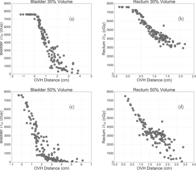
Using the nominal OVH to quantify anatomy, the DVH-OVH correlation showed a negatively linear relationship in both OARs for each fractional volume observed. Bladder dose showed a strong anticorrelation with distance, having a mean R = -0.79 over the four fractional volumes analyzed. Rectum dose also showed a strong anticorrelation with distance, having a mean R = -0.82 (Table 3). Figure 5 shows each nominal DVH-OVH scatter plot associated with each Pearson correlation coefficient listed in Table 3.

Table 3: Pearson correlation coefficients between nominal OVH distances and DVH dose-volumes of the bladder and rectum. An absolute value greater than 0.7 indicates a strong linear correlation with a maximum value of 1.

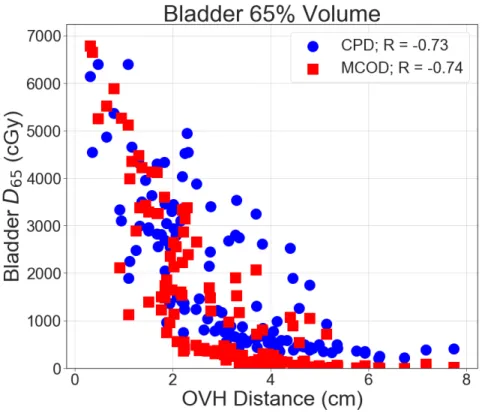
Dose-Volume DVH-OVH R Bladder D30 -0.92 D50 -0.83 D65 -0.74 D80 -0.66 Mean -0.79 Rectum D30 -0.94 D50 -0.86 D65 -0.78 D80 -0.70 Mean -0.82

The variation in distance-to-dose correlation across patients can be seen in Figure 5. For example, the reader is directed to the DVH-OVH plot for 65% of the rectum (Figure 5 (f)), where the range of D65 for an OVH distance of 2 cm was 643 to 3011 cGy. This spread in dose of greater

(36)

than 2300 cGy for a given OVH distance is consistent with previous studies and illustrates the motivation of the present study.52,63,70

Figure 5: Nominal DVH-OVH correlations for 30, 50, 65, and 80% dose-volumes of the bladder (a, c, e, g) and rectum (b, d, f, h).

(a) (b)

(37)

(Figure 5 continued)

2.2.2 SECOND-ORDER FACTORS

Each previously investigated second-order factor was introduced as a variable into the nominal DVH-OVH correlation for each fractional volume of the bladder and rectum via a color bar. The variables were visually inspected via these color bar scatter plots to assess relational dependence between the second-order factors and dose for the fractional OAR volumes. Of all the factors studied, only the in-field OAR volume showed any noticeable influence on OAR dose, as seen in Figure 6 (c) and (d). The data indicated that, as the in-field OAR volume increases, the dose-volume value for the associated OAR also increases. This trend was observed in all scatter plots for

3011 cGy

643 cGy

(e) (f)

(38)

every fractional volume DVH-OVH of the bladder and the rectum. For the other factors investigated, no such trends were noted (see Figure 6 (a) and (b)).

Figure 6: Sample color scatter plots for qualitative review of dependence on the examined second-order factors. There is no visible relationship between dose and PTV volume for neither 65% of the bladder (a) nor the rectum (b). When analyzing in-field OAR volume however, a clear relationship with D65 for the bladder (c) and rectum (d) can be seen.

Pearson correlation coefficients between second-order factors and bladder and rectum dose-volumes are listed in Table 4. Of the six variables inspected, only in-field OAR volume showed a strong correlation with OAR dose for both the bladder (mean R = 0.86) and the rectum (mean R = 0.76). The in-field OAR volume had a correlation coefficient of greater than 0.7 for each bladder and rectum dose-volume, except for D30 of the rectum. While the dOVH was strongly correlated

(a) (b)

(39)

with D30 (R = 0.75) and D50 (R = 0.74) of the rectum, the in-field OAR volume resulted in a

stronger correlation with rectum dose overall. This indicates in-field OAR volume had the strongest correlation with OAR dose out of the evaluated factors, confirming the qualitative indications. Table 4: Pearson correlation coefficients between each second-order factor and DVH dose-volumes for the bladder and rectum. The mean Pearson coefficient over the four fractional volumes is also listed. Only the in-field OAR volume was strongly correlated (mean greater than 0.7) for both the bladder and rectum.

Dose-Volume dOVH _DoseRx _VolumePTV _VolumeBladder _VolumeRectum In-field OAR _Volume Bladder D30 0.62 -0.44 0.50 -0.53 0.20 0.90 D50 0.56 -0.41 0.41 -0.55 0.19 0.88 D65 0.52 -0.41 0.39 -0.52 0.17 0.85 D80 0.48 -0.43 0.38 -0.53 0.18 0.83 Mean 0.54 -0.42 0.42 -0.53 0.19 0.86 Rectum D₃₀ 0.75 -0.60 0.77 0.16 -0.11 0.56 D50 0.74 -0.49 0.67 0.05 -0.07 0.74 D65 0.67 -0.43 0.56 -0.07 -0.02 0.87 D80 0.55 -0.53 0.60 -0.11 -0.09 0.85 Mean 0.68 -0.51 0.65 < 0.01 -0.05 0.76 2.2.3 IMPROVED DVH-OVH CORRELATION

The distance-to-dose correlation showed improvement when the in-field OAR volume was accounted for in the computation of the OVH (Table 5). For the bladder, the in-field OVH

strengthened the mean correlation coefficient from -0.79 to -0.85 over the four fractional volumes. While for the rectum, the mean correlation strengthened from -0.82 to -0.86. This increase in

correlation strength was especially noticeable at the 80% fractional volume level for both the bladder and rectum, where the 80% bladder DVH-OVH R strengthened from -0.66 to -0.77 and the value for 80% rectum improved from -0.70 to -0.86.

An illustrative example of the differences between the DVH-OVH correlations using the nominal OVH versus the in-field OVH can be seen in Figure 7. Accounting for the in-field OAR volume in the OVH computation resulted in an improvement in the distance-to-dose correlation for

(40)

65% and 80% of the bladder (Figure 7 (a) and (c) respectively) and rectum (Figure 7 (b) and (d) respectively). It is important to reiterate that the decrease in data points for the higher fractional in-field OAR volumes is due to certain database patients not meeting the given in-in-field OAR volume threshold.

Table 5: Pearson correlation coefficients between in-field OVH distances and DVH dose-volumes of the bladder and rectum. The correlation coefficients between the nominal OVH distances and DVH dose-volumes from Table 3 are also listed for comparison. Note that n refers to the number of database patients with in-field OAR volumes greater than or equal to the given dose-volume.

DVH-OVH R

Dose-Volume Nominal OVH In-field OVH Bladder D₃₀ -0.92 -0.91 (n = 108) D50 -0.83 -0.88 (n = 76) D65 -0.74 -0.85 (n = 52) D80 -0.66 -0.77 (n = 35) Mean -0.79 -0.85 Rectum D30 -0.94 -0.93 (n = 124) D50 -0.86 -0.84 (n = 117) D65 -0.78 -0.82 (n = 90) D80 -0.70 -0.86 (n = 49) Mean -0.82 -0.86

With regards to the representative example of the distance-to-dose correlation variation at 65% of the rectum introduced earlier (referencing Figure 5 (f)), Figure 7 (b) shows the reduction in the dose spread at an OVH distance of 2 cm from using the in-field OVH method. The group of patients with rectum D65 less than 10 Gy have very low doses to the rectum, most likely due to

having less than 65% of the rectum inside the treatment fields. The removal of these patients using the in-field OVH term reduces the dose spread at the OVH distance of 2 cm from over 20 Gy with the nominal OVH method to less than 10 Gy.