SFB 649 Discussion Paper 2005-020
A Dynamic
Semiparametric Factor
Model for Implied
Volatility String
Dynamics
Matthias R. Fengler*
Wolfgang K. Härdle**
Enno Mammen***
* Trading & Derivatives, Sal. Oppenheim jr. & Cie., Germany ** CASE – Center for Applied Statistics and Economics,
Humboldt-Universität zu Berlin, Germany
*** Department of Economics, University of Mannheim, Germany
This research was supported by the Deutsche
Forschungsgemeinschaft through the SFB 649 "Economic Risk". http://sfb649.wiwi.hu-berlin.de ISSN 1860-5664 SFB 649, Humboldt-Universität zu Berlin
S
FB
6
4
9
E
C
O
N
O
M
I
C
R
I
S
K
B
E
R
L
I
N
A Dynamic Semiparametric Factor Model for
Implied Volatility String Dynamics
∗
Matthias R. Fengler
†Trading & Derivatives, Sal. Oppenheim jr. & Cie. Untermainanlage 1, 60329 Frankfurt am Main, Germany
Wolfgang K. H¨
ardle
CASE – Center for Applied Statistics and Economics
Humboldt-Universit¨at zu Berlin,
Spandauer Straße 1, 10178 Berlin, Germany
Enno Mammen
Department of Economics, University of Mannheim L 7, 3–5, 68131 Mannheim, Germany
March 6, 2005
∗We gratefully acknowledge financial support by the Deutsche Forschungsgemeinschaft and the
Sonder-forschungsbereich 649 “ ¨Okonomisches Risiko”.
†Corresponding author: [email protected], TEL ++49 69 7134 5512, FAX ++49 69 7134 9
A Dynamic Semiparametric Factor Model for Implied Volatility String Dynamics
Abstract
A primary goal in modelling the implied volatility surface (IVS) for pricing and hedging aims at reducing complexity. For this purpose one fits the IVS each day and applies a principal component analysis using a functional norm. This approach, however, neglects the degenerated string structure of the implied volatility data and may result in a modelling bias. We propose a dynamic semiparametric factor model (DSFM), which approximates the IVS in a finite dimensional function space. The key feature is that we only fit in the local neighborhood of the design points. Our approach is a combination of methods from functional principal component analysis and backfitting techniques for additive models. The model is found to have an approximate 10% better performance than a sticky moneyness model. Finally, based on the DSFM, we devise a generalized vega-hedging strategy for exotic options that are priced in the local volatility framework. The generalized vega-hedging extends the usual approaches employed in the local volatility framework.
JEL classification codes: C14, G12
Keywords: smile, local volatility, generalized additive model, backfitting, functional principal
1
Introduction
Successful trading, hedging and risk managing of option portfolios crucially depends on the accuracy of the underlying pricing models. Consequently, new valuation approaches are
continuously developed in departing from the foundations of option theory laid by Black
and Scholes (1973), Merton(1973) and Harrison and Kreps(1979), and existing models are
refined. However, despite these pervasive developments, the model of Black and Scholes
(1973) remains a pivot in modern financial theory and an important benchmark for more
sophisticated models, be it from a theoretical or practical point of view.
The popularity of the Black and Scholes (BS) model is likely due to its clear and easy-to-communicate set of assumptions. Based on the geometric Brownian motion for the under-lying asset price dynamics, and continuous trading in a complete and frictionless market, simple closed form solutions for plain vanilla calls and puts are derived: given the current un-derlying price at time, the option’s strike price, its expiry date the prevailing riskless interest rate, and an estimate of the (expected) market volatility, option prices are straightforward to compute.
The crucial parameter in option valuation by BS is the market volatility. Since it is unknown,
one studiesimpliedvolatility, which is derived by inverting the BS formula for a cross section
of options with different strikes and maturities traded at the same point in time. As is visible
in the left panel of Figure 1 for May 2, 2000 (i.e. 20000502, a notation we will use from
now on), implied volatilities display a remarkable curvature across the strike dimension, and – albeit to a lesser degree – a term structure across time to maturity. For a given time to
maturity the phenomenon is called smile or smirk. This dependence given by the mapping
ˆ
σt : (κ, τ)→σˆt(κ, τ), where κdenotes the strike dimension scaled in moneyness and τ time
to maturity, is called implied volatility surface (IVS). The indext denotes time-dependence.
Apparently, it is in contrast with the BS framework in which volatility is assumed to be a constant across strikes, time to maturity and also time.
There is a considerable amount of literature which aims at reconciling this empirical antag-onism with financial theory. Generally speaking, this can be achieved by including another degree of freedom into option pricing models: well-known examples are stochastic volatility
IVS Ticks 20000502 0.16 0.28 0.40 0.51 0.63 0.56 0.71 0.87 1.02 1.18 0.26 0.32 0.38 0.44 0.50 Data Design 0.4 0.5 0.6 0.7 0.8 0.9 1 1.1 1.2 1.3 1.4 Moneyness 0 0.1 0.2 0.3 0.4 0.5 0.6 0.7 Time to maturity
Figure 1: Left panel: call and put implied volatilities observed on 2nd May, 2000. Right
panel: data design on 2nd May, 2000, ODAX. Lower left axis is moneyness κ def= K/Ft, where Ft denotes the futures price, lower right axis time to maturity
models (Hull and White, 1987; Stein and Stein, 1991; Heston, 1993), models with jump
diffusions (Bates,1996a,b), or models building on general L´evy processes, e.g. based on the
inverse Gaussian (Barndorff-Nielsen, 1997), and generalized hyperbolic distribution (
Eber-lein and Prause,2002). These approaches capture the smile and term structure phenomena
and the complexity of its dynamics to some extent, as is documented for instance in Das
and Sundaram (1999) and Bergomi (2004).
Nevertheless, the BS model and the IVS enjoy much popularity. Partly, this is due to the fact that the IVS is derived from a cross-section of option prices at a specific point in time. Therefore, unlike estimates based on historical data, the IVS is a widely accepted state
variable that reflects current market sentiments, Bakshi et al. (2000). More importantly,
however, the IVS plays a decisive role in trading: market makers at plain vanilla desks con-tinuously monitor and update the IVS they trade on; and exotic derivatives trader calibrate their pricing engines with an estimate of the IVS. This is particularly obvious for the pricing
Der-Model fit 20000502 0.14 0.23 0.32 0.41 0.50 0.80 0.88 0.96 1.04 1.12 -1.46 -1.30 -1.14 -0.98 -0.82
Semiparametric factor model fit 20000502
0.14 0.23 0.32 0.41 0.50 0.80 0.88 0.96 1.04 1.12 -1.47 -1.31 -1.16 -1.00 -0.85
Figure 2: Nadaraya-Watson estimator and DSFM fit for 20000502. Bandwidths for both
estimates h1 = 0.03 for the moneyness and h2 = 0.04 for the time to maturity dimension. Axes as in the left panel.
man and Kani (1994), they are in wide-spread use in form of the efficient implementations
by Andersen and Brotherton-Ratcliffe (1997) and Dempster and Richards (2000). Thus, refined statistical model building of the IVS determines vitally the accuracy of applications in trading and risk-management.
In modelling the IVS one faces two main challenges. First, the data have a degenerated
design: due to institutional conventions, observations of the IVS occur only for a small number of maturities such as one, two, three, six, nine, twelve, 18, and 24 months to expiry on the date of issue. Consequently, implied volatilities appear in a row like pearls strung on
a necklace, Figure 1, or, in short: as ‘strings’. This pattern is visible in the right panel of
Figure 1, which plots the data design as seen from top. Options belonging to the same string
have a common time to maturity. As time passes, the strings move through the maturity axis towards expiry while changing levels and shape in a random fashion. Second, also in the moneyness dimension, the observation grid does not cover the desired estimation grid at any point in time. Thus, even when the data sets are huge, for a large number of cases implied volatility observations are missing for certain sub-regions of the desired estimation
grid. This is particularly virulent when transaction based data are used. However, despite their appearance as strings, implied volatilities are thought as being the observed structure of a smooth surface. This is because in practice one needs to price and hedge OTC options whose expiry dates do not coincide with the expiry dates of the options that are traded at the futures exchange.
For the semi- or nonparametric approximations to the IVS that have been promoted by
A¨ıt-Sahalia and Lo (1998), Rosenberg (2000), A¨ıt-Sahalia et al. (2001b), Cont and da Fonseca
(2002),Fengler et al.(2003) and Fengler and Wang(2003), this design may pose difficulties.
For illustration, consider in Figure 2 (left panel) the fit of a standard Nadaraya-Watson
estimator. Bandwidths are h1 = 0.03 for the moneyness and h2 = 0.04 for the time to
maturity dimension (measured in years). The fit appears very rough, and there are huge holes in the surface, since the bandwidths are too small to ‘bridge’ the gaps between the maturity strings. In order to remedy this deficiency one would need to strongly increase the bandwidths which may induce a large bias. Moreover, since the design is time-varying, the bandwidths would also need to be adjusted anew for each trading day, which complicates
daily applications. Parametric models, e.g. as inShimko(1993),An´e and Geman(1999), and
Brockhaus et al. (2000, Chap. 2) among others, are less affected by these data limitations, but appear to offer too little functional flexibility to capture the salient features of IVS patterns. Thus, parametric estimates may as well be biased.
In this paper we provide a new principal component approach for modelling the IVS: the complex dynamic structure of the IVS is captured by a low-dimensional dynamic semipara-metric factor model (DSFM) with time-varying coefficients. The IVS is approximated by unknown basis functions moving in a finite dimensional function space. The dynamics can be understood by using vector autoregression (VAR) techniques on the time-varying co-efficients. Contrary to earlier studies, we will use only finite dimensional fits to implied
volatilities which are obtained in the local neighborhood of strikes and maturities, for which
implied volatilities are recorded at the specific day. Surface estimationanddimension
reduc-tion is achieved in one single step. Our technology can be seen as a combinareduc-tion of funcreduc-tional principal component analysis, nonparametric curve estimation and backfitting for additive models.
time, i.e. for fitting, the information contained in other observations dates in the sample
is exploited, see Section 2 for the details. This is possible due to the expiry effect which
is a unique feature present IVS data. As explained, this effect insures that observations gradually move through the entire observation space. To our knowledge there do not exist estimation techniques that explicitly take advantage of this effect.
To introduce our model, let us denote the implied volatility by Yi,j, where the index i is
the number of the day (i = 1, . . . , I), and j = 1, . . . , Ji is an intra-day numbering of the
option traded on day i. The observations Yi,j are regressed on two-dimensional covariables
Xi,j that contain moneynessκi,j and maturityτi,j. Moneyness is defined asκi,j
def
= Ki,j/Ft,i,j,
i.e. strike Ki,j divided by the underlying futures price Ft,i,j at timeti,j. We also considered
the one-dimensional case in which Xi,j =κi,j. However, since modelling the entire surface is
more interesting, we will present results for this case only. The DSFM is given by:
m0(Xi,j) + L
X
l=1
βi,lml(Xi,j), (1)
where ml are smooth basis functions (l = 0, . . . , L). The IVS is approximated by a weighted
sum of smooth functions ml with weights βi,l depending on time i. The factor loading
βi def
= (βi,1, . . . βi,L)> forms an unobserved multivariate time series. By fitting model (1),
to the implied volatility strings we obtain approximations βbi. We argue that the VAR
estimation based on βbi is asymptotically equivalent to estimation based on the unobserved
βi. A justification for this is given in Borak et al. (2005) where the relations to Kalman
filtering are discussed.
Lower dimensional approximations of the IVS based on principal components analysis (PCA)
have been used in Zhu and Avellaneda (1997) andFengler et al. (2002) in an application to
the term structure of implied volatilities, and in Skiadopoulos et al. (1999) and Alexander
(2001) in studies across strikes. Fengler et al. (2003) use a common principal components
approach to study several maturity groups across the IVS simultaneously, while Cont and
da Fonseca (2002) propose a functional PCA perspective for the IVS. All these approaches treat the IVS as a stationary process, and do not take particular care for the degenerated
Our modelling approach is also different in the following respect: for instance, in Cont and da Fonseca (2002) the IVS is fitted on a grid for each day. Afterwards a PCA using a functional norm is applied to the surfaces. This treatment follows the usual functional PCA
approach as described in Ramsay and Silverman (1997). In our approach the IVS is fitted
each day at the observed design points Xi,j. This leads to a minimization with respect to
functional norms that depend on timei. We loose a nice feature of the usual functional PCA
though: when fitting the data forLand L∗ =L+ 1, the linear space spanned bymb0, . . . ,mbL
may not be contained in the one spanned by mb∗0, . . . ,mb∗L∗. On the other hand we only make
use of values of the implied volatilities at regions where they are observed. This avoids bias effects caused by global daily fits used in standard functional PCAs.
The model can be employed in several respects: given the estimated functions mbl and the
time series βb, scenario simulations of potential IVS scenarios are straightforward. They can
help to give a more accurate assessment of market risk than previous approaches. Worst case scenarios can be identified, which provide additional supervision tools to risk managers. For trading, the model may be used as a tool of short range IVS prediction or as an input factor
in the local volatility models such as the one by Andersen and Brotherton-Ratcliffe(1997).
As we will demonstrate, the model also offers a unified tool to traders for vega hedging of complex option positions in a local volatility setting.
The paper is organized as follows: in the following section, implied volatilities are described
and the DSFM is introduced. In Section 3 the model is applied to DAX option implied
volatilities for the sample period 1998 to May 2001. Section 4 discusses the hedging of
complex option positions in the local volatility setting, Section 5 concludes.
2
Time-dependent implied volatility modelling
2.1
The semiparametric factor model
Implied volatilities are derived from the BS option pricing formula for European calls and
puts, Black and Scholes (1973). European style calls and puts are contingent claims on an
and max(K −St,0), respectively, for a strike K at a given expiry day T. The asset price
process St in the BS model is assumed to be a geometric Brownian motion. The BS option
pricing formula for calls is given by:
CtBS(St, K, τ, r, σ) = StΦ(d1)−e−rτKΦ(d2), (2) where d1 def = log(St/K)+(r+12σ2)τ σ√τ and d2 def = d1−σ √
τ. Φ(·) denotes the cumulative distribution
function of the standard normal distribution, τ def= T −t time to maturity of the option,
r the riskless interest rate over the option’s life time, and σ the diffusion coefficient of the
Brownian motion. Put prices Pt are obtained via the put-call-parityCt−Pt =St−e−τ rK.
The only unknown parameter in (2) is the volatility parameter σ. Given observed market
prices ˜Ct, implied volatility ˆσ is defined by:
CtBS(St, K, τ, r,σˆ)−C˜t= 0 . (3)
Due to monotonicity of the BS price in σ, there exists a unique solution ˆσ >0. Define the
moneyness metric κt
def
= K/Ft, where Ft denotes the futures price time t.
In the dynamic factor model, we regress Yi,j
def
= log{σˆi,j(κ, τ)} on Xi,j = (κi,j, τi,j) via
nonparametric methods. We work with log-implied volatility data, since the data appear less skewed and potential outliers are scaled down after taking logs. This is common practice
in the IVS literature, see e.g. Zhu and Avellaneda (1997) and Cont and da Fonseca (2002).
In order to estimate the nonparametric componentsmland the state variables βi,l in (1), we
borrow ideas from fitting additive models as in Stone (1986), Hastie and Tibshirani (1990)
and Horowitz et al. (2002). Our research is related to functional coefficient models such as Cai et al. (2000). Other semi- and nonparametric factor models include Connor and Linton (2000), Gouri´eroux and Jasiak (2001), Fan et al. (2003), and Linton et al. (2003).
Nonparametric techniques are now broadly used in option pricing, e.g. Broadie et al.(2000a),
Broadie et al. (2000b), A¨ıt-Sahalia et al. (2001a), and A¨ıt-Sahalia and Duarte (2003).
The estimatesmbl, (l = 0, . . . , L) andβbi,l(i= 1, . . . , I; l= 1, . . . , L) are defined as minimizers
of the following least squares criterion (βbi,0
def = 1): I X i=1 Ji X j=1 Z ( Yi,j− L X l=0 b βi,lmbl(u) )2 Kh(u−Xi,j) du . (4)
Here, Kh denotes a two-dimensional product kernel,Kh(u) =kh1(u1)×kh2(u2), h= (h1, h2),
based on a one-dimensional kernel kh(v)
def
= h−1k(h−1v).
In (4) the minimization runs over all functions mbl : R2 → R and all values βbi,l ∈ R. For
illustration let us consider the case L = 0 : implied volatilities Yi,j are approximated by a
surface mb0 that does not depend on time i. In this degenerated case, mb0(u) =
P
i,jKh(u−
Xi,j)Yi,j/Pi,jKh(u−Xi,j), which is the Nadaraya-Watson estimate based on the pooled
sample of all days.
Using (4), the implied volatility surfaces are approximated by surfaces moving in an L
-dimensional affine function space {mb0+
PL
l=1αlmbl: α1, . . . , αL∈R}.The estimates mbl are
not uniquely defined: they can be replaced by functions that span the same affine space.
In order to respond to this problem, we select mbl such that they are orthogonal. This will
facilitate the interpretation of the functions, as shall be seen in Section 3 and 4.
Replacing in (4)mblbymbl+δgwith arbitrary functionsg and taking derivatives with respect
to δ yields, for 0≤l0 ≤L: I X i=1 Ji X j=1 ( Yi,j− L X l=0 b βi,lmbl(u) ) b βi,l0Kh(u−Xi,j) = 0. (5)
Furthermore, by replacing βbi,l by βbi,l+δ in (4) and again taking derivatives with respect
to δ, we get for 1 ≤l0 ≤L and 1≤i≤I:
Ji X j=1 Z ( Yi,j− L X l=0 b βi,lmbl(u) ) b ml0(u)Kh(u−Xi,j) du= 0. (6)
Introducing the following notation, for 1 ≤i≤I
b pi(u) = 1 Ji Ji X j=1 Kh(u−Xi,j), (7) b qi(u) = 1 Ji Ji X j=1 Kh(u−Xi,j)Yi,j , (8)
we obtain from (5)-(6), for 1≤l0 ≤L,1≤i≤I: I X i=1 Jiβbi,l0 b qi(u) = I X i=1 Ji L X l=0 b βi,l0βbi,l b pi(u)mbl(u), (9) Z b qi(u)mbl0(u) du = L X l=0 b βi,l Z b pi(u)mbl0(u)mbl(u) du . (10)
We calculate the estimates by iterative use of (9) and (10). We start by initial valuesβb
(0) i,l for
b
βi,l. A possible choice of the initial βbcould correspond to fits of surfaces that are piecewise
constant on time intervals I1, . . . , IL. This means, for l = 1, .., L, put βb
(0)
i,l = 1 (for i ∈ Il),
and βb
(0)
i,l = 0 (for i /∈ Il). Here I1, ..., IL are pairwise disjoint subsets of {1, ..., I} and
L
S
l=1 Il
is a strict subset of {1, ..., I}. For r ≥0, we put βb
(r)
i,0 = 1. Define the matrix B
(r)(u) by its elements: B(r)(u)l,l0 def = I X i=1 Jiβb (r−1) i,l0 βb (r−1) i,l bpi(u), 0≤l, l 0 ≤ L , (11)
and introduce a vector Q(r)(u) with elements
Q(r)(u)l def = I X i=1 Jiβb (r−1) i,l qbi(u), 0≤l ≤L . (12)
In the r-th iteration the estimate mb = (mb0, . . . ,mbL)
> is given by:
b
m(r)(u) =B(r)(u)−1Q(r)(u). (13)
This update step is motivated by (9). The values of βb are updated in the r-th cycle as
follows: define the matrix M(r)(i)
M(r)(i)l,l0 def = Z b pi(u)mb (r) l0 (u)mb (r) l (u)du , 1≤l, l 0 ≤ L , (14)
and define a vector S(r)(i)
S(r)(i)l def = Z b qi(u)mbl(u) du− Z b pi(u)mb (r) 0 (u)mb (r) l (u) du , 1≤l ≤L . (15) Motivated by (10), put b βi,1(r), ...,βb (r) i,L > =M(r)(i)−1S(r)(i). (16)
The algorithm is run until only minor changes occur. In the implementation, we choose a
grid of points and calculate mbl at these points. In the calculation of M(r)(i) and S(r)(i),
we replace the integral by a Riemann sum approximation using the values of the integrated functions at the grid points.
As discussed above, mbl and βbi,l are not uniquely defined. Therefore, we orthogonolize
b
m0, . . . ,mbL in L
2(ˆp), where ˆp(u) = I−1PI
i=1pˆi(u), such that
PI
i=1βbi,12 is maximal, and
given βbi,1, b m0,mb1, PI i=1βb 2
i,2 is maximal, and so forth. These aims can be achieved by the
following two steps: first replace
b m0 by mb new 0 = mb0−γ >Γ−1 b m , b m by mbnew = Γ−1/2m ,b b βi,1 .. . b βi,L by b βnew i,1 .. . b βnew i,L = Γ1/2 b βi,1 .. . b βi,L + Γ−1γ , (17) where mb = (mb1, . . . ,mbL) >
and the (L×L) matrix Γ = R mb(u)mb(u)>pˆ(u)du, or for
clar-ity, Γ = (Γl,l0), with Γl,l0 = R
b
ml(u) mbl0(u)ˆp(u)du. Finally, we have γ = (γl), with γl =
R b
m0(u)mbl(u)ˆp(u)du.
Note that by applying (17), mb0 is replaced by a function that minimizes
R b
m20(u)ˆp(u)du.
This is evident because mb0 is orthogonal to the linear space spanned by mb1, . . .mbL. By the
second equation of (17), mb1, . . . ,mbL are replaced by orthonormal functions in L
2(ˆp).
In a second step, we proceed as in PCA and define a matrix B with Bl,l0 =PI
i=1βbi,lβbi,l0 and
calculate the eigenvalues of B, λ1 > . . . > λL, and the corresponding eigenvectors z1, . . . zL.
Put Z = (z1, . . . , zL). Replace b m by mbnew = Z> b m , (18) (i.e. mbnew l =z > l mb),and b βi,1 .. . b βi,L by b βnew i,1 .. . b βnew i,L = Z> b βi,1 .. . b βi,L . (19)
After application of (18) and (19) the orthonormal basis mb1, . . . ,mbL is chosen such that PI
i=1βb2i,1 is maximal, and – given βbi,1,mb0,mb1 – the quantity
PI
i=1βbi,22 is maximal, . . ., i.e.
b
m1 is chosen such that as much as possible is explained by βbi,1
b
m1. Next mb2 is chosen to
achieve maximum explanation by βbi,1
b
m1+βbi,2 b
m2, and so forth.
The functions mbl are not eigenfunctions of an operator as in usual functional PCA. This is
because we use a different norm, namely R f2(u)ˆpi(u)du, for each day. Through the norming
procedure the functions are chosen as eigenfunctions in an L-dimensional approximating
lin-ear space. The L-dimensional approximating spaces are not necessarily nested for increasing
L. For this reason the estimates cannot be calculated by an iterative procedure that starts
by fitting a model with one component, and that uses the old L−1 components in the
iteration step from L−1 toLto fit the next component. The calculation of mb0, . . . ,mbLhas
to be fully redone for different choices of L.
3
The dynamic factors of the DAX index IVS
3.1
Data description and preparation
Our data set contains tick statistics on DAX futures contracts and DAX index options traded at the futures exchange EUREX in Frankfurt/Main in the period from January 1998 to May 2001. Both futures price and option price data are contract based data, i.e. each single contract is registered together with its price, contract size, and time of settlement up to a hundredth second. Interest rate data in daily frequency, i.e. one-, three-, six-, and twelve-months FIBOR rates for the years 1998–1999 and EURIBOR rates for the period
2000–2001, were obtained from Thomson Financial Datastream. Interest rate data were
linearly interpolated to approximate the riskless interest rate for the option specific time to maturity.
In a first step, we recover the DAX index values. To this end, we group to each option price
observation the futures price Ft of the nearest available futures contract, which was traded
within a one minute interval around the observed option. The futures price observation was taken from the most heavily traded futures contract on the particular day, usually the
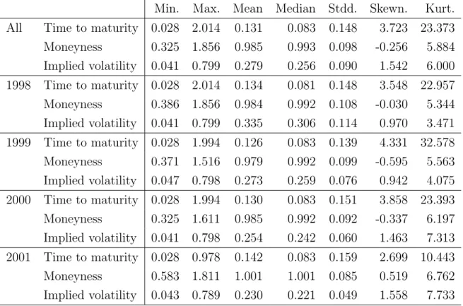
three-Min. Max. Mean Median Stdd. Skewn. Kurt.
All Time to maturity 0.028 2.014 0.131 0.083 0.148 3.723 23.373
Moneyness 0.325 1.856 0.985 0.993 0.098 -0.256 5.884 Implied volatility 0.041 0.799 0.279 0.256 0.090 1.542 6.000 1998 Time to maturity 0.028 2.014 0.134 0.081 0.148 3.548 22.957 Moneyness 0.386 1.856 0.984 0.992 0.108 -0.030 5.344 Implied volatility 0.041 0.799 0.335 0.306 0.114 0.970 3.471 1999 Time to maturity 0.028 1.994 0.126 0.083 0.139 4.331 32.578 Moneyness 0.371 1.516 0.979 0.992 0.099 -0.595 5.563 Implied volatility 0.047 0.798 0.273 0.259 0.076 0.942 4.075 2000 Time to maturity 0.028 1.994 0.130 0.083 0.151 3.858 23.393 Moneyness 0.325 1.611 0.985 0.992 0.092 -0.337 6.197 Implied volatility 0.041 0.798 0.254 0.242 0.060 1.463 7.313 2001 Time to maturity 0.028 0.978 0.142 0.083 0.159 2.699 10.443 Moneyness 0.583 1.811 1.001 1.001 0.085 0.519 6.762 Implied volatility 0.043 0.789 0.230 0.221 0.049 1.558 7.733
Table 1: Summary statistics on the data base from 199801 to 200105 for the IVS application
in Section 3.2, entirely and on an annual basis. 2001 is from 200101 to 200105, only.
months contract. The no-arbitrage price of the underlying index in a frictionless market
without dividends is given by St=Fte−rTF ,t(TF−t), whereSt andFt denote the index and the
futures price respectively, TF the futures contract’s maturity date, andrT,t the interest rate
with maturity T −t.
The DAX index is a capital weighted performance index, i.e. dividends less corporate tax
are reinvested into the index, Deutsche B¨orse (2002). Therefore, dividend payments should
have no impact on index options. However, when only the interest rate discounted futures price is used to recover implied volatilities by inverting the BS formula, implied volatilities of calls and puts can differ significantly. To accommodate for this fact we apply a correction
algorithm that is described in Appendix B. The entire data set is stored in the financial
database MD*base, www.mdtech.de, maintained at the Center for Applied Statistics and Economics (CASE), Berlin.
Since the data are transaction based and may contain misprints or outliers, a filter is applied before estimating the model: observations with implied volatility less than 4% and bigger than 80% are dropped. Furthermore, we disregard all observations having a maturity less than ten days. After this filtering, the entire number of observations is more than 4.48 million contracts, i.e. is around 5 200 observations per day.
Table 1 gives a short summary of our IVS data. Most heavy trading occurs in short term
contracts, as is seen from the difference between median and mean of the term structure distribution of observations as well as from its skewness. Median time to maturity is 30 days (0.083 years). Across moneyness the distribution is slightly negatively skewed. Mean implied volatility over the sample period is 27.9%.
3.2
Empirical evidence
We model log-implied volatility Yi,j on Xi,j = (κi,j, τi,j)>. The grid covers in moneyness
κ ∈ [0.80,1.20] and in time to maturity τ ∈ [0.05,0.5] measured in years. We employ
L = 3 basis functions, which capture around 96.0% of the variations in the IVS. To our
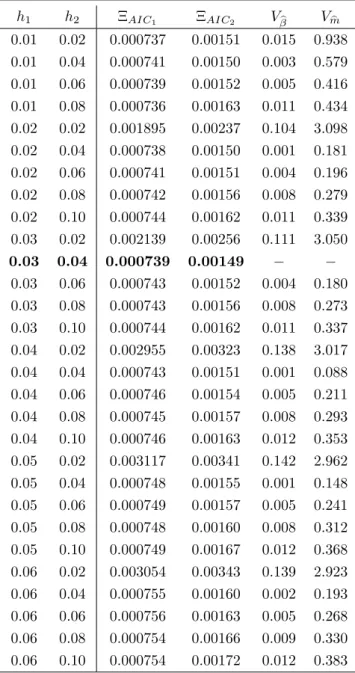
understanding, this is of sufficiently high accuracy. The bandwidths are h1 = 0.03 for
moneyness and h2 = 0.04 for time to maturity. This choice is justified by Table 3.2 which
presents the estimates for the two Akaike information criteria (AIC) that are explained in
detail in AppendixA. Both criterion functions become very flat near the minimum. Criterion
ΞAIC2 assumes its global minimum in the neighborhood of h
∗ = (0.03,0.04)>, which is why
we opt for these bandwidths. In being able to choose these small bandwidths, the strength of our modelling approach is demonstrated: indeed, the bandwidth in the time to maturity dimension is so small that in a fit of a particular day, data belonging to contracts with two
adjacent time to maturities do not enter together pbi(u) in (7) andqbi(u) in (8). In fact, for a
given u0, the quantitiespbi(u0) andqbi(u
0
) are zero most of the time, and only assume positive
values for dates i, when observations are in the local neighborhood ofu0. Of course, during
the entire observation period I, it is mandatory that observations for eachu for some dates
5 10 15 20 25 Number of Iterations -4 -3 -2 -1 0 1 2 3 4 5 6 log_10(Fitting Criterion) Average density 0.14 0.23 0.32 0.41 0.50 0.80 0.88 0.96 1.04 1.12 11.75 23.36 34.96 46.56 58.16
Figure 3: Left panel: convergence in the IVS models. Solid line shows the L1, the dotted
line the L2 measure of convergence. Total number of iterations is 25. Right panel: average density pˆ(u) = I−1PI
i=1pˆi(u). Bandwidths are h1 = 0.03 for moneyness and h2 = 0.04 for time to maturity.
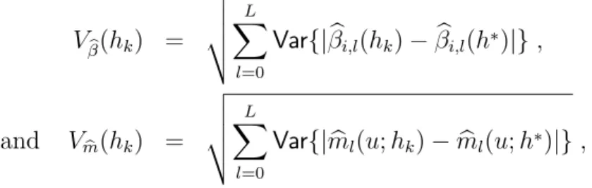
the basis functions change relative to the optimal bandwidth h∗. We compute:
V b β(hk) = v u u t L X l=0
Var{|βbi,l(hk)−βbi,l(h∗)|}, (20)
and Vmb(hk) = v u u t L X l=0 Var{|mbl(u;hk)−mbl(u;h ∗)|}, (21)
where hk runs over the values given in Table 3.2, and Var(x) denotes the variance of x. It
is seen that changes in mb are 10 to 100 times higher in magnitude than those for βb. This
corroborates the approximation in (32) that treats the factor loadings as known. In Figure3
we display an L1- and an L2-convergence measure of the algorithm, see Appendix A for
definitions. Convergence is achieved quickly, and we stop the iterations after 25 cycles, when
the L2 was less than 10−5.
h1 h2 ΞAIC1 ΞAIC2 Vβb Vmb 0.01 0.02 0.000737 0.00151 0.015 0.938 0.01 0.04 0.000741 0.00150 0.003 0.579 0.01 0.06 0.000739 0.00152 0.005 0.416 0.01 0.08 0.000736 0.00163 0.011 0.434 0.02 0.02 0.001895 0.00237 0.104 3.098 0.02 0.04 0.000738 0.00150 0.001 0.181 0.02 0.06 0.000741 0.00151 0.004 0.196 0.02 0.08 0.000742 0.00156 0.008 0.279 0.02 0.10 0.000744 0.00162 0.011 0.339 0.03 0.02 0.002139 0.00256 0.111 3.050 0.03 0.04 0.000739 0.00149 − − 0.03 0.06 0.000743 0.00152 0.004 0.180 0.03 0.08 0.000743 0.00156 0.008 0.273 0.03 0.10 0.000744 0.00162 0.011 0.337 0.04 0.02 0.002955 0.00323 0.138 3.017 0.04 0.04 0.000743 0.00151 0.001 0.088 0.04 0.06 0.000746 0.00154 0.005 0.211 0.04 0.08 0.000745 0.00157 0.008 0.293 0.04 0.10 0.000746 0.00163 0.012 0.353 0.05 0.02 0.003117 0.00341 0.142 2.962 0.05 0.04 0.000748 0.00155 0.001 0.148 0.05 0.06 0.000749 0.00157 0.005 0.241 0.05 0.08 0.000748 0.00160 0.008 0.312 0.05 0.10 0.000749 0.00167 0.012 0.368 0.06 0.02 0.003054 0.00343 0.139 2.923 0.06 0.04 0.000755 0.00160 0.002 0.193 0.06 0.06 0.000756 0.00163 0.005 0.268 0.06 0.08 0.000754 0.00166 0.009 0.330 0.06 0.10 0.000754 0.00172 0.012 0.383
Table 2: Bandwidth selection via AIC as given in (33) and (34) for different choices of h:
h1 refers to moneyness andh2 to time to maturity measured in years; the bandwidth chosen is highlighted in bold. In all cases L = 3. Vβb and V
b
m measure the change in βb and b
m as functions of h relative the optimal bandwidth h∗ = (0.03,0.04)>, compare (20) and (21).
display the invariant function mb0, since it essentially is the zero function of the affine space
fitted by the data: both mean and median are zero up to 10−2 in magnitude. We believe
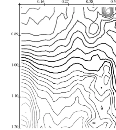
this to be estimation error. The remaining functions exhibit more interesting patterns: mb1
in Figure 4 is positive throughout, and mildly concave. There is little variability across
the term structure. Since this function belongs to the weights with highest variance, we
interpret it as the time dependent mean of the (log)-IVS, i.e. a shift effect. Function mb2,
depicted in Figure 5, changes sign around the at-the-money region, which implies that the
smile deformation of the IVS is exacerbated or mitigated by this eigenfunction. Hence we
consider this function as a moneyness slope effect of the IVS. Finally,mb3 is positive for the
very short term contracts, and negative for contracts with maturity longer than 0.1 years,
Figure 6. Thus, a positive weight in βb3 lowers short term implied volatilities and increases
long term implied volatilities: mb3 generates the term structure dynamics of the IVS, it
provides a term structure slope effect. These observations are line with the results of earlier
studies on the IVS, Skiadopoulos et al. (1999),Cont and da Fonseca (2002), and Fengler et
al.(2003). It is important to remark that the eigenfunctions appear quite rough, which is due
the small bandwidths we use here for demonstration. Depending on the specific application,
for instance the one we consider in Section 4it may be advisable to employ somewhat larger
bandwidths.
To appreciate the power of the DSFM, we inspect again the case of 20000502. In Figure 7,
we compare a Nadaraya-Watson estimator (left panel) with the DSFM (right panel). In the
first case, the bandwidths are increased to h= (0.06,0.25)> in order to remove all holes and
excessive variation in the fit, while for the latter the bandwidths are kept ath= (0.03,0.04)>.
While both fits look similar at first sight, the differences are best visible when both cases
are contrasted for each time to maturity string separately, Figures 8 to 11. Generally, the
standard Nadaraya-Watson fit exhibits a strong directional bias, especially in the wings. The DSFM is not entirely unbiased either, but clearly the fit is superior.
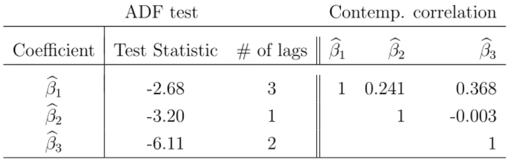
Figure 12 shows the time series of βb1 to βb3 and their correlograms. Summary statistics
are given in Table 3 and contemporaneous correlation in the right part of Table 4. The
ADF tests at the 5% level, left part of Table 4, indicate a unit root for βb1 and βb2. Thus,
one may model first differences of the first two loading series together with the levels of
b
0.14 0.23 0.32 0.41 0.50 0.80 0.88 0.96 1.04 1.12 0.70 0.84 0.99 1.14 1.28 0.89 1.00 1.10 1.20 0.16 0.27 0.38 0.50
Figure 4: Factor mb1 in the left panel (moneyness lower left axis, lower right axis time to
maturity). Right panel shows contour plots of this function (moneyness left axis, time to maturity top). Lines are thick for positive level values, thin for negative ones. The gray scale becomes increasingly lighter the higher the level in absolute value. Stepwidth between contour lines is 0.028, estimated from ODAX data 199801-200105.
Min. Max. Mean Median Stdd. Skewn. Kurt.
b β1 -1.541 -0.462 -1.221 -1.260 0.206 1.101 4.082 b β2 -0.075 0.106 0.001 0.002 0.034 0.046 2.717 b β3 -0.144 0.116 0.002 -0.001 0.025 0.108 5.175
Table 3: Summary statistics on (βb1,βb2,βb3)> from Section3.2.
significant, one may estimate the levels of the loading series in a rich VAR model. We opt for
the latter choice and use a VAR(2) model, Table 5. The estimation also includes a constant
and two dummy variables, assuming the value one right at those days and one day after, when the corresponding IV observations of the minimum time to maturity string (10 days to expiry) were to be excluded from the estimation of the DSFM. This is to capture possible seasonality effects introduced from the data filter.
0.14 0.23 0.32 0.41 0.50 0.80 0.88 0.96 1.04 1.12 -1.39 -0.36 0.67 1.70 2.73 0.89 1.00 1.10 1.20 0.16 0.27 0.38 0.50
Figure 5: Factor mb2 in the left panel (moneyness lower left axis, lower right axis time to
maturity). Right panel shows contour plots of this function (moneyness left axis, time to maturity top). Lines are thick for positive level values, thin for negative ones. The gray scale becomes increasingly lighter the higher the level in absolute value. Stepwidth between contour lines is 0.225, estimated from ODAX data 199801-200105.
and dummies are weakly significant, but not shown for the sake of clarity. As is seen
all factor loadings follow AR(2) processes. There are also a number of remarkable cross dynamics. Exploiting these cross dynamics is vital for the model’s performance, as shall be seen in the subsequent prediction contest.
3.3
Prediction contest
We now study the prediction performance of our model compared with a benchmark model.
Model comparisons that have been conducted, for instance by Bakshi et al. (1997),Dumas
et al. (1998), and Bates (2000), often reveal that simple trader models perform better than more sophisticated models. These models used by professionals simply assert that today’s implied volatility is tomorrow’s implied volatility. There are two versions: the sticky strike assumption pretends that implied volatility is constant at fixed strikes. The sticky moneyness
0.14 0.23 0.32 0.41 0.50 0.80 0.88 0.96 1.04 1.12 -3.66 -2.15 -0.63 0.88 2.40 0.89 1.00 1.10 1.20 0.16 0.27 0.38 0.50
Figure 6: Factor mb3 in the left panel (moneyness lower left axis, lower right axis time to
maturity). Right panel shows contour plots of this function (moneyness left axis, time to maturity top). Lines are thick for positive level values, thin for negative ones. The gray scale becomes increasingly lighter the higher the level in absolute value. Stepwidth between contour lines is 0.240, estimated from ODAX data 199801-200105.
Model fit 20000502 0.14 0.23 0.32 0.41 0.50 0.80 0.88 0.96 1.04 1.12 -1.47 -1.31 -1.16 -1.00 -0.85
Semiparametric factor model fit 20000502
0.14 0.23 0.32 0.41 0.50 0.80 0.88 0.96 1.04 1.12 -1.47 -1.31 -1.16 -1.00 -0.85
Figure 7: Nadaraya-Watson estimator with h = (0.06,0.25)> and DSFM with h =
Traditional string fit 20000502, 17 days to exp. 0.8 0.9 1 1.1 1.2 Moneyness -1.6 -1.4 -1.2 -1
Individual string fit 20000502, 17 days to exp.
0.8 0.9 1 1.1 1.2 Moneyness -1.6 -1.4 -1.2 -1
Figure 8: Bias comparison of the Nadaraya-Watson estimator with h = (0.06,0.25)> (left
panel) and the semi-parametric factor model with h = (0.03,0.04)> (right panel) for the 17 days to expiry data (black bullets) on 20000502.
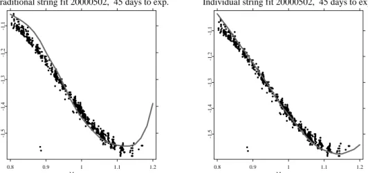
Traditional string fit 20000502, 45 days to exp.
0.8 0.9 1 1.1 1.2 Moneyness -1.5 -1.4 -1.3 -1.2 -1.1
Individual string fit 20000502, 45 days to exp.
0.8 0.9 1 1.1 1.2 Moneyness -1.5 -1.4 -1.3 -1.2 -1.1
Figure 9: Bias comparison of the Nadaraya-Watson estimator with h = (0.06,0.25)> (left
panel) and the semi-parametric factor model with h = (0.03,0.04)> (right panel) for the 45 days to expiry data (black bullets) on 20000502.
Traditional string fit 20000502, 80 days to exp. 0.8 0.9 1 1.1 1.2 Moneyness -1.5 -1.4 -1.3 -1.2 -1.1
Individual string fit 20000502, 80 days to exp.
0.8 0.9 1 1.1 1.2 Moneyness -1.5 -1.4 -1.3 -1.2 -1.1
Figure 10: Bias comparison of the Nadaraya-Watson estimator with h = (0.06,0.25)> (left
panel) and the semi-parametric factor model with h = (0.03,0.04)> (right panel) for the 80 days to expiry data (black bullets) on 20000502.
Traditional string fit 20000502, 136 days to exp.
0.8 0.9 1 1.1 1.2 Moneyness -1.6 -1.5 -1.4 -1.3 -1.2 -1.1
Individual string fit 20000502, 136 days to exp.
0.8 0.9 1 1.1 1.2 Moneyness -1.6 -1.5 -1.4 -1.3 -1.2 -1.1
Figure 11: Bias comparison of the Nadaraya-Watson estimator with h = (0.06,0.25)> (left
panel) and the semi-parametric factor model with h= (0.03,0.04)> (right panel) for the 136 days to expiry data (black bullets) on 20000502.
basis coeff. 1 1998 1999 2000 2001 Time -1.5 -1 -0.5 basis coeff. 2 1998 1999 2000 2001 Time -0.05 0 0.05 0.1 basis coeff. 3 1998 1999 2000 2001 Time -0.1 -0.05 0 0.05 0.1
basis coeff. 1: ACF
0 5 10 15 20 25 30 lag 0 0.5 1 acf
basis coeff. 2: ACF
0 5 10 15 20 25 30 lag 0 0.5 1 acf
basis coeff. 3: ACF
0 5 10 15 20 25 30 lag 0 0.5 1 acf
Figure 12: Upper panel: time series of weights (βb1,βb2,βb3)>. Lower panel: autocorrelation
functions.
We use the sticky moneyness model as our benchmark. There are two reasons for this choice:
first, from a methodological point of view, as has been shown byBalland(2002) and Daglish
et al. (2003), the sticky strike rule as an assumption on the stochastic process governing implied volatilities, is not consistent with the existence of a smile. The sticky moneyness rule, however, can be. Second, since we estimate our model in terms of moneyness, sticky moneyness rule is most natural.
Our methodology in comparing prediction performance is as follows: as presented in
Sec-tion 3.2, the resulting times series of latent factors βbi,l is replaced by a times series model
with fitted values βei,l(ˆθ) based on βbi0,l with i0 ≤ i−1 ,1 ≤ l ≤ L, where ˆθ is a vector of
estimated coefficients seen in Table5. As in Section2, we employ a variant of ΞAIC1 based on
thefittedvalues as an asymptotically unbiased estimate of mean square prediction error. The
ADF test Contemp. correlation
Coefficient Test Statistic # of lags βb1 βb2 βb3
b β1 -2.68 3 1 0.241 0.368 b β2 -3.20 1 1 -0.003 b β3 -6.11 2 1
Table 4: Left part: ADF tests on βb1 to βb3 for the full IVS model, intercept included in each
case. Third column gives the number of lags included in the ADF regression. For the choice of lag length, we started with four lags, and subsequently deleted lag terms, until the last lag term became significant at least at a 5% level. MacKinnon critical values for rejecting the hypothesis of a unit root are -2.87 at 5% significance level, and -3.44 at 1% significance level. Right part: contemporaneous correlation matrix.
three equations plus a constant and two dummy variables), see Appendix A.
This criterion, denoted by ΞeAIC, is compared with the squared one-day prediction error of
the sticky moneyness (StM) model:
ΞStM def = N−1 I X i Ji X j (Yi,j−Yi−1,j0)2 . (22)
In practice, since one hardly observes Yi,j at the same moneyness as in i −1, Yi−1,j0 is
obtained via a localized interpolation of the previous day’s smile. Time to maturity effects are neglected, and observations, the previous values of which are lost due to expiry, are deleted from the sample. Running the model comparison shows:
ΞStM = 0.00476 versus ΞeAIC = 0.00439 .
Thus, the model comparison reveals that the DSFM is approximate 10% better than the
sticky moneyness model. This is a substantial improvement given the high variance in
Equation
Dependent variable βb1,i βb2,i βb3,i
b β1,i−1 0.978 -0.009 0.047 [24.40] [-1.21] [ 3.70] b β1,i−2 0.004 0.012 -0.047 [ 0.08] [ 1.63] [-3.68] b β2,i−1 0.182 0.861 0.134 [ 0.92] [ 23.88] [ 2.13] b β2,i−2 -0.129 0.109 -0.126 [-0.65] [ 3.03] [-2.01] b β3,i−1 0.115 -0.019 0.614 [ 0.97] [-0.89] [ 16.16] b β3,i−2 -0.231 0.030 0.248 [-1.96] [ 1.40] [ 6.60] ¯ R2 0.957 0.948 0.705 F-statistic 2405.273 1945.451 258.165
Table 5: Estimation results of an VAR(2) of the factor loadings βbi. t-statistics given in
brackets, R¯2 denotes the adjusted coefficient of determination. The estimation includes an intercept and two dummy variables (both not shown), which assume the value one right at those days and one day after, when the corresponding IV observations of the minimum time to maturity string (10 days to expiry) were to be excluded from the estimation of the DSFM.
4
Hedging in local volatility models using the DSFM
Local volatility models are one-factor models, i.e. it is assumed that the asset price dynamics are governed by the stochastic differential equation
dSt St
=µ dt+σ(St, t)dWt, (23)
where Wt is a Brownian motion, µ denotes the drift, and σ(St, t) the local volatility
employed to calibrate the local volatility function to the market. Then, the BS partial dif-ferential equation with generalized volatility function is solved for pricing the exotic options,
Andersen and Brotherton-Ratcliffe (1997) and Dempster and Richards (2000). Therefore,
unlike to the BS model, prices depend on the entire IVS, and not simply on the implied
volatility at a specific strike. In consequence, the notion of vega hedging needs to be gener-alized. A usual attempt to respond to this problem, is to define a so called ‘parallel-shift-vega’ which corresponds to the sensitivity of the option price with respect to a parallel shift of the whole IVS. It is calculated via bumping the IVS by a certain factor and computing the difference quotient. From our empirical analysis, however, it is obvious that the IVS displays much more sophisticated dynamics as is manifest in the moneyness slope and term structure slope effects. While an up-and-down shift of the IVS may be the most important factor, the parallel-shift-vega leaves the slope and term structure risks, which the exotic option is exposed to, unhedged. Depending on the specific payoff profile of the option, these risks, however, can be of substantial size. For instance, for down-and-out puts, the probability of hitting the barrier is very much determined by the slope of the smile. In this case, it is desirable to hedge the slope risks of the IVS.
The DSFM gives a decomposition of the IVS into its most important factors. For path-dependent options, we therefore propose to define the hedge in terms of these factors. More precisely, given the decomposition
ˆ σt(κ, τ) = exp L X l=0 b βt,lmbl ! , (24)
the β1-greek, ∂β∂1, defines the sensitivity of the option with respect to up-and-down shifts of
the (log)-IVS. Theβ2-greek, ∂β∂2, is a slope-shift-vega of the (log)-IVS, and so on. For setting
up a hedge, one needs to define portfolios HP1, HP2, . . . consisting of plain vanilla options
that have approximately the same first order expansion in terms of these beta-greeks. Given the hedge-ratios the residual delta risk is hedged with the underlying. The particular nature of the hedge portfolio depends on the exotic option to be hedged, but may also depend on general targets in risk management such as to reduce gamma risks.
To make our approach more precise, we concentrate on the two-factor case with two hedge
portfoliosHP1 andHP2 and the aforementioned down-and-out putPdo. First, one computes
instance via a difference quotient. The hedge ratios a1 and a2 for a ‘beta-neutral’ hedge are
obtained by solving the linear system of equations:
∂HP1 ∂β1 ∂HP2 ∂β1 ∂HP1 ∂β2 ∂HP2 ∂β2 a1 a2 = ∂Pdo ∂β1 ∂Pdo ∂β2 . (25)
Equations (25) give an immediate suggestion of how to choose the hedge portfolios.
Obvi-ously, it is desirable to define HP1 and HP2 such that they have maximum exposure to β1
and β2, respectively, since in this case, ∂HP∂β21 ≈ 0 and ∂HP∂β12 ≈ 0. For the down-and-out put
considered here, a natural choice is to use a portfolio of at-the-money plain vanilla options
in HP1, and in HP2 a vega-neutral risk reversal. A risk reversal is a short position in an
out-of-the-money plain vanilla call and a long position in an out-of-the-money put (or vice versa). The value of a risk reversal primarily responds to changes in the wings of the IVS and by selecting the appropriate strikes, it can be set up in a vega-neutral way.
We expect this ‘beta-hedging’ approach to be superior to the usual parallel-shift-vega for a number of reasons: first, the parallel-shift-vega corresponds to a hedge in the DSFM with
only one factor. Second, it mimics the rich structure of the factor surface ofmb1that is visible
in Figure 4, only in an insufficient way. Finally, beta-hedging allows to reduce the slope and
curvature risks. Conducting a comparative hedging exercise along the lines of Bakshi et al.
(1997) and Dumas et al. (1998) is topic of our ongoing research on the DSFM.
5
Conclusion
In this study we present a modelling approach to the implied volatility surface (IVS) that takes care of the particular discrete string structure of implied volatility data. The technique comes from functional PCA and backfitting in additive models. Unlike other studies, our ansatz is tailored to the degenerated design of implied volatility data by fitting basis functions in the local neighborhood of the design points only. We thus avoid bias effects. Using transactions based DAX index implied volatility data from 1998 to May 2001, we recover a number of basis functions generating the dynamics of a single implied volatility string and surface. The functions may be intuitively interpreted as level, term structure and moneyness
slope effects, and a term structure twist effect, known from earlier literature. We study the time series properties of parameters weights and complete the modelling approach by fitting vector autoregressive models. A three-dimensional VAR(2) describes IVS dynamics best. In a prediction contest, we compare the performance of our model with a sticky moneyness model. Finally, based on these factors, we devise a generalized vega-hedging strategy for exotic options that are priced in the local volatility framework. The generalized vega-hedging extends the usual parallel-shift vega approaches that are typically employed.
There are two important topics for further research. First, from a practical point of view the DSFM must be put into a contest of competing hedging strategies for some prime examples of exotic options, such as barriers. Second, from a theoretical point of view, the DSFM has a natural relation with Kalman filtering. Kalman filtering is a way to recursively find
solutions to discrete-data linear filtering problems, Kalman (1960). For, writing our model
more compactly as:
Θp(B)βi = ui (26)
Yi,j = m0(Xi,j) + L
X
l=1
βi,lml(Xi,j) +εi,j , (27)
where ui and εi,j are noise, and Θp(B)
def
= 1−θ1B −θ2B2. . .−θpBp denotes a polynomial
of order p in the backshift operator B, we receive the typical state-space representation.
Equation (27) is called the state equationdepending on a parameter vector θ. It relates the
(unobservable) stateiof the system to the previous stepi−1. Themeasurement equation(27)
relates the state to the measurement, the IVS in our case. The difference to our work is
that the time series modelling of βi is done after recovering it. This integrated approach is
References
A¨ıt-Sahalia, Y. and Duarte, J. (2003). Nonparametric option pricing under shape restrictions,
Journal of Econometrics 116: 9–47.
A¨ıt-Sahalia, Y. and Lo, A. (1998). Nonparametric estimation of state-price densities implicit
in financial asset prices,Journal of Finance 53: 499–548.
A¨ıt-Sahalia, Y., Bickel, P. J. and Stoker, T. M. (2001a). Goodness-of-fit tests for regression
using kernel methods, Journal of Econometrics 105: 363–412.
A¨ıt-Sahalia, Y., Wang, Y. and Yared, F. (2001b). Do options markets correctly price the
probabilities of movement of the underlying asset?, Journal of Econometrics102: 67–110.
Alexander, C. (2001). Principles of the skew, RISK 14(1): S29–S32.
Andersen, L. B. G. and Brotherton-Ratcliffe, R. (1997). The equity option volatility smile:
An implicit finite-difference approach, Journal of Computational Finance 1(2): 5–37.
An´e, T. and Geman, H. (1999). Stochastic volatility and transaction time: An activity-based
volatility estimator, Journal of Risk 2(1): 57–69.
Bakshi, G., Cao, C. and Chen, Z. (1997). Empirical performance of alternative option pricing
models, Journal of Finance 52(5): 2003–2049.
Bakshi, G., Cao, C. and Chen, Z. (2000). Do call and underlying prices always move in the
same direction?, Review of Financial Studies 13(3): 549–584.
Balland, P. (2002). Deterministic implied volatility models, Quantitative Finance 2: 31–44.
Barndorff-Nielsen, O. E. (1997). Normal inverse Gaussian distributions and stochastic
volatil-ity modelling, Scandinavian Journal of Statistics 24: 1–13.
Bates, D. S. (1996a). Dollar jump fears, 1984:1992, distributional anomalies implicit in
currency futures options, Journal of International Money and Finance 15: 65–93.
Bates, D. S. (1996b). Jumps and stochastic volatility: Exchange rate processes implicit in
Bates, D. S. (2000). Post-’87 crash fears in the S&P 500 futures option market, Journal of Econometrics 94(1-2): 181–238.
Bergomi, L. (2004). Smile dynamics, RISK17(9): 117–123.
Black, F. and Scholes, M. (1973). The pricing of options and corporate liabilities, Journal
of Political Economy 81: 637–654.
Borak, S., Fengler, M. R., H¨ardle, W. and Mammen, E. (2005). Semiparametric state space
factor models, CASE Discussion Paper, Humboldt-Universit¨at zu Berlin.
Broadie, M., Detemple, J., Ghysels, E. and Torr`es, O. (2000a). American options with
stochastics dividends and volatility: A nonparametric investigation, Journal of
Econo-metrics 94: 53–92.
Broadie, M., Detemple, J., Ghysels, E. and Torr`es, O. (2000b). Nonparametric estimation
of American options exercise boundaries and call prices, Journal of Economic Dynamics
and Control 24: 1829–1857.
Brockhaus, O., Farkas, M., Ferraris, A., Long, D. and Overhaus, M. (2000). Equity
deriva-tives and market risk models, Risk Books, London.
Cai, Z., Fan, J. and Yao, Q. (2000). Functional-coefficient regression models for nonlinear
time series, Journal of the American Statistical Association 95: 941–956.
Connor, G. and Linton, O. (2000). Semiparametric estimation of a characteristic-based
factor model of stock returns, Technical report, LSE, London.
Cont, R. and da Fonseca, J. (2002). The dynamics of implied volatility surfaces,Quantitative
Finance 2(1): 45–60.
Daglish, T., Hull, J. C. and Suo, W. (2003). Volatility surfaces: Theory, rules of thumb,
and empirical evidence, Working paper, J. L. Rotman School of Management, University
of Toronto.
Das, S. and Sundaram, R. (1999). Of smiles and smirks: A term-structure perspective,
Dempster, M. A. H. and Richards, D. G. (2000). Pricing American options fitting the smile,
Mathematical Finance 10(2): 157–177.
Derman, E. (1999). Regimes of volatility, RISK12(4): 55–59.
Derman, E. and Kani, I. (1994). Riding on a smile, RISK 7(2): 32–39.
Deutsche B¨orse (2002). Leitfaden zu den Aktienindizes der Deutschen B¨orse, 4.3 edn,
Deutsche B¨orse AG, 60284 Frankfurt am Main.
Dumas, B., Fleming, J. and Whaley, R. E. (1998). Implied volatility functions: Empirical
tests, Journal of Finance 80(6): 2059–2106.
Dupire, B. (1994). Pricing with a smile, RISK 7(1): 18–20.
Eberlein, E. and Prause, K. (2002). The generalized hyperbolic model: Financial derivatives
and risk measures, in H. Geman, D. Madan, S. Pliska and T. Vorst (eds), Mathematical
Finance - Bachelier Congress 2000, Springer Verlag, Heidelberg, New York, pp. 245 – 267.
Fan, J., Yao, Q. and Cai, Z. (2003). Adaptive varying-coefficient linear models, J. Roy.
Statist. Soc. B. 65: 57–80.
Fengler, M. R. and Wang, Q. (2003). Fitting the smile revisited: A least squares kernel
estimator for the implied volatility surface,SfB 373 Discussion Paper 2003-25,
Humboldt-Universit¨at zu Berlin.
Fengler, M. R., H¨ardle, W. and Schmidt, P. (2002). Common factors governing VDAX
move-ments and the maximum loss, Journal of Financial Markets and Portfolio Management
16(1): 16–29.
Fengler, M. R., H¨ardle, W. and Villa, C. (2003). The dynamics of implied volatilities: A
common principle components approach, Review of Derivatives Research6: 179–202.
Gouri´eroux, C. and Jasiak, J. (2001). Dynamic factor models, Econometrics Review
20(4): 385–424.
Hafner, R. and Wallmeier, M. (2001). The dynamics of DAX implied volatilities,
H¨ardle, W., Klinke, S. and M¨uller, M. (2000). Xplore – Learning Guide, Springer Verlag, Heidelberg.
Harrison, J. and Kreps, D. (1979). Martingales and arbitrage in multiperiod securities
markets, Journal of Economic Theory 20: 381–408.
Hastie, T. and Tibshirani, R. (1990). Generalized additive models, Chapman and Hall,
London.
Heston, S. (1993). A closed-form solution for options with stochastic volatility with
appli-cations to bond and currency options, Review of Financial Studies 6: 327–343.
Horowitz, J., Klemela, J. and Mammen, E. (2002). Optimal estimation in additive models,
Preprint.
Hull, J. and White, A. (1987). The pricing of options on assets with stochastic volatilities,
Journal of Finance 42: 281–300.
Kalman, R. E. (1960). A new approach to linear filtering and prediction problems,
Trans-actions of the ASME–Journal of Basic Engineering 82: 35–45.
Linton, O., Nguyen, T. and Jeffrey, A. (2003). Nonparametric estimation of single factor
Heath-Jarrow-Morton term structure models and a test for path independence, Technical
report, LSE, London.
Merton, R. C. (1973). Theory of rational option pricing, Bell Journal of Economics and
Management Science4(Spring): 141–183.
Ramsay, J. O. and Silverman, B. W. (1997). Functional Data Analysis, Springer, New York,
Berlin.
Rosenberg, J. (2000). Implied volatility functions: A reprise,Journal of Derivatives7: 51–64.
Shimko, D. (1993). Bounds on probability, RISK 6(4): 33–37.
Skiadopoulos, G., Hodges, S. and Clewlow, L. (1999). The dynamics of the S&P 500 implied
Stein, E. M. and Stein, J. C. (1991). Stock price distributions with stochastic volatility: An
analytic approach, Review of Financial Studies 4: 727–752.
Stone, C. J. (1986). The dimensionality reduction principle for generalized additive models,
The Annals of Statistics 14: 592–606.
Zhu, Y. and Avellaneda, M. (1997). An E-ARCH model for the term-structure of implied
A
Model selection
The model selection for the DSFM entails the the choice of the model sizeL, the bandwidth
vector h, and measuring the convergence of the backfitting algorithm. This is detailed in
this appendix.
For the model size we use the residual sum of squares for different L:
RV(L)def= PI i PJi j n Yi,j −PLl=0βbi,l b ml(Xi,j) o2 PI i PJi j (Yi,j −Y¯)2 , (28)
where ¯Y denotes the overall mean of the observations. The quantity 1−RV(L) is the portion
of variance explained in the approximation, and Lcan be increased until a sufficiently high
level of fitting accuracy is achieved. This is a common selection method also in ordinary PCA.
For a data-driven choice of bandwidths, we propose a weighted AIC. We use a weighted
criterion, since the distribution of observations is very unequal, Figure 3. This can lead
to nonconvexity in the criterion and typically results into inacceptably small bandwidths, see Fengler et al. (2003) for a first description of this problem. It is natural to punish the
criterion in areas where the distribution is sparse. For a given weight function w, consider:
4(m0, . . . , mL) def = E 1 N X i,j {Yi,j − L X l=0
βi,lml(Xi,j)}2w(Xi,j), (29)
for functionsm0, . . . , mL. The expectation operator is denoted byE. We choose bandwidths
such that4(mb0, . . . ,mbL) is minimal. According to the AIC this is asymptotically equivalent
to minimizing: ΞAIC1 def = 1 N X i,j {Yi,j − L X l=0 b βi,lmbl(Xi,j)} 2w(X i,j) exp 2L NKh(0) Z w(u)du . (30)
Alternatively, one may consider the computationally more easy criterion:
ΞAIC2 def = 1 N X i,j {Yi,j− L X l=0 b βi,lmbl(Xi,j)} 2 exp 2L NKh(0) R w(u)du R w(u)p(u)du . (31)
Putting w(u) def= 1, delivers the common AIC. This, however, does not take into account the quality of the estimation at the boundary regions or in regions where data are sparse,
since in these regions p(u) is small. We propose to choose w(u)def= p−1(u), which gives equal
weight everywhere as can be seen by the following considerations:
4(m0, . . . , mL) = E 1 N X i,j ˆ ε2w(Xi,j) + E 1 N X i,j " L X l=0
βi,l{ml(Xi,j)−mbl(Xi,j)} #2 w(Xi,j) ≈ σε2 Z w(u)p(u)du + 1 N X i,j Z " L X l=0 βi,l{ml(u)−mbl(u)} #2 w(u)p(u)du , (32)
where ε denotes the residual and σ2
ε def
= Var(ε).
The two criteria finally are:
ΞAIC1 def = 1 N X i,j {Yi,j− L X l=0 b βi,lmbl(Xi,j)} 2pˆ(X i,j) exp 2L NKh(0) Z 1 ˆ p(u)du , (33) and ΞAIC2 def = 1 N X i,j {Yi,j− L X l=0 b βi,lmbl(Xi,j)} 2 exp 2L NKh(0)µ −1 λ Z 1 ˆ p(u)du , (34)
where µλ denotes the Lebesgue measure of the design set.
Under some regularity conditions, the AIC is an asymptotically unbiased estimate of the mean averaged square error (MASE). In our setting it would be consistent if the density of
Xi,j did not depend on day i. Due to the irregular design, this is an unrealistic assumption.
For this reason, ΞAIC1 and ΞAIC2 estimate a weighted versions of MASE.
In our AIC the penalty term does not punish for the number parameters βbi,l that are
em-ployed to model the time series. This can be neglected because we will use a finite dimensional
smoothing penalty term. For the prediction contest, however, we use a penalty term that
takes care of the specific parametric model of βe(θ). More precisely, for the model contest,
we use criterion ΞAIC1 with w(u)
def
= 1. This results in:
e ΞAIC def = N−1 I X i Ji X j ( Yi,j− L X l=0 e βi,l(ˆθ)mbl(Xi,j) )2 ×exp 2 L NKh(0)µλ+ 2 dim(θ) N . (35)
Thus, we penalize for the dimension of the model.
Clearly, the choice of hand L are not independent. From this point of view, one may think
about minimizing (33) or (34) over both parameters. However, our practical experience
shows that for a given L, changes in the criteria from variation in h is small, compared to
variation in L for a givenh. To reduce the computational burden, we use (28) to determine
model size L, and then (33) and (34) to optimize h for a given L.
Convergence of the iterations is measured by
Qk(r) def = I X i=1 Z L X l=0 b βi(r)mb(r)l (u)−βb (r−1) i mb (r−1) l (u) k du . (36)
The rth cycle of the estimation is denoted by (r). Here, we approximate the integral by
simple sums over the estimation grid. Putting k = 1,2, we have an L1- and an L2-measure
B
Dividend correction scheme
Here, we explain the dividend correction algorithm. To illustrate the aforementioned
div-idend problem consider Figure 13. There, for the calculation of implied volatilities, the
DAX spot price has been approximated by simply discounting the DAX futures price. As is visible, implied volatilities of calls (crosses) and puts (circles) fall apart, and violate the
put-call-parity. As an explanation, Hafner and Wallmeier (2001) argue that the individual
tax scheme of the marginal investor can be different from the one actually assumed to com-pute the DAX index. Consequently, the net dividend for this investor is higher or lower than the one used for the index computation. This discrepancy, which the authors call ‘difference dividend’, has the same impact as a dividend payment for an unprotected option, i.e. it
drives a wedge into the option prices and hence into implied volatilities. Denote by ∆Dt,T
the timeT value of this difference dividend incurred betweent andT. Consider the dividend
adjusted formula for a futures price:
Ft=erF(TF−t)St−∆Dt,TF , (37)
and the dividend adjusted put-call parity:
Ct−Pt =St−∆Dt,THe
−rH(TH−t)−e−rH(TH−t)K (38)
with TH denoting the call’sCt and the put’s Pt maturity date. Inserting equation (37) into
(38) yields Ct−Pt =e−rF(TF−t)Ft+ ∆Dt,TH,TF −e −rH(TH−t)K , (39) where ∆Dt,TH,TF def = ∆Dt,TFe −rF(TF−t)−∆D t,THe
−rH(TH−t) is the desired difference dividend.
The ‘adjusted’ index level
˜
St=e−rF(TF−t)Ft+ ∆Dt,TH,TF (40)
is that index level, which ties put and call implied volatilities exactly to the same levels when used in the inversion of the BS formula.
For an estimate of ∆ ˆDt,TH,TF, pairs of puts and calls of the strikes and same maturity
Implied Volatility Surface Ticks 0.08 0.11 0.14 0.17 0.20 0.72 0.82 0.92 1.02 1.12 0.25 0.29 0.32 0.35 0.39
Figure 13: IVS ticks on April 4, 2000, derived from futures prices that are interest rate
discounted only. Put implied volatility are circles, call implied volatility crosses.
∆Dt,TH,TF is derived from equation (39). To ensure robustness ∆ ˆDt,TH,TF is estimated by the
median of all ∆Dt,TH,TF of the pairs for a given maturity at day t. Implied volatilities are
recovered by inverting the BS formula using the corrected index value ˜St = Fte−rF(TF−t)+
∆ ˆDt,TH,TF. Note that ∆Dt,TH,TF = 0, when TH = TF. Indeed, when calculated also in this
case, ∆ ˆDt,TH,TF proved to be very small (compared with the index value), which supports
the validity of this approach. The described procedure is applied on a daily basis throughout the entire data set from 199801 to 200105.
In Figure 14, we present the data after correcting the discounted futures price with an
implied difference dividend ∆ ˆDt = (10.3,5.0,1.9)>, where the first entry refers to 16 days,
the second to 45 days and the third to 73 days to maturity. Implied volatilities of puts and calls converge two one single string, while the concavity of the put volatility smile is
remedied, too. Note that the overall level of implied volatility string is not altered through
Implied Volatility Surface Ticks 0.08 0.11 0.14 0.17 0.20 0.72 0.82 0.92 1.02 1.12 0.26 0.29 0.33 0.36 0.40
Figure 14: IVS ticks on April 4, 2000, derived from futures prices that are interest rate
discounted and corrected with the implied difference dividend. Put implied volatility are circles, call implied volatility crosses.
SFB 649 Discussion Paper Series
For a complete list of Discussion Papers published by the SFB 649, please visit http://sfb649.wiwi.hu-berlin.de.
001 "Nonparametric Risk Management with Generalized Hyperbolic Distributions" by Ying Chen, Wolfgang Härdle and Seok-Oh Jeong, January 2005.
002 "Selecting Comparables for the Valuation of the European Firms" by Ingolf Dittmann and Christian Weiner, February 2005.
003 "Competitive Risk Sharing Contracts with One-sided Commitment" by Dirk Krueger and Harald Uhlig, February 2005.
004 "Value-at-Risk Calculations with Time Varying Copulae" by Enzo Giacomini and Wolfgang Härdle, February 2005.
005 "An Optimal Stopping Problem in a Diffusion-type Model with Delay" by Pavel V. Gapeev and Markus Reiß, February 2005. 006 "Conditional and Dynamic Convex Risk Measures" by Kai
Detlefsen and Giacomo Scandolo, February 2005.
007 "Implied Trinomial Trees" by Pavel Čížek and Karel Komorád, February 2005.
008 "Stable Distributions" by Szymon Borak, Wolfgang Härdle and Rafal Weron, February 2005.
009 "Predicting Bankruptcy with Support Vector Machines" by Wolfgang Härdle, Rouslan A. Moro and Dorothea Schäfer, February 2005.
010 "Working with the XQC" by Wolfgang Härdle and Heiko Lehmann, February 2005.
011 "FFT Based Option Pricing" by Szymon Borak, Kai Detlefsen and Wolfgang Härdle, February 2005.
012 "Common Functional Implied Volatility Analysis" by Michal Benko and Wolfgang Härdle, February 2005.
013 "Nonparametric Productivity Analysis" by Wolfgang Härdle and Seok-Oh Jeong, March 2005.
014 "Are Eastern European Countries Catching Up? Time Series Evidence for Czech Republic, Hungary, and Poland" by Ralf Brüggemann and Carsten Trenkler, March 2005.
015 "Robust Estimation of Dimension Reduction Space" by Pavel
Čížek and Wolfgang Härdle, March 2005.
016 "Common Functional Component Modelling" by