Simplicial Complexes From Graphs Toward Graph Persistence

SCUOLA DI SCIENZE

Corso di Laurea Magistrale in Matematica

SIMPLICIAL COMPLEXES FROM GRAPHS

TOWARDS GRAPH PERSISTENCE

Tesi di Laurea Magistrale in Topologia Algebrica

Relatore:

Prof. Massimo Ferri

Correlatore:

Dott. Mattia G. Bergomi

Presentata da:

Lorenzo Zuffi

Sessione III

Introduzione 3

Introduction 5

Preliminary standard definitions 9

1 Simplicial compexes built from a graph 15

1.1 Abstract . . . 15

1.2 Complex of Cliques . . . 17

1.3 Complex of Independent sets . . . 19

1.4 Complex of Neighbours . . . 21

1.5 Acyclic subsets . . . 25

1.5.1 Complex of induced acyclic subgraphs . . . 25

1.5.2 Complex of acyclic subsets of the edge set . . . 25

1.5.3 Complex of removable acyclic subgraphs . . . 26

1.6 Complex of enclaveless sets . . . 28

1.6.1 Enclaveless sets implementations . . . 29

2 Graph persistence 33 2.1 Persistent homology: a brief introduction . . . 33

2.2 Persistent homologic properties for simplicial complexes from a graph 36 2.2.1 Case study: edge filtrations on𝐾4 . . . 37

2.2.2 Filtration on edge-induced subgraphs: a simple example . . . . 48

2.2.3 Complexes from acyclic subsets and persistent homology . . . 48

2.3 Other Persistent properties: blocks and edge-blocks . . . 51

2.3.1 The persistent block number . . . 52

2.3.2 The persistent edge-block number . . . 53

3 Other methods to build simplicial complexes 57 3.1 The complex ofk-cyclesCy𝑗 ,𝑘(𝐺 ) . . . 57

3.2 The complex of connected cliques . . . 59 1

Appendix

63

Lo scopo di questo elaborato `e di esplorare diversi metodi attraverso i quali ottenere complessi simpliciali a partire da un grafo, suggerendo alcuni risultati originali in tal senso. L’obiettivo `e introdurre, in un articolo di prossima pubblicazione, una general-izzazione della teoria dell’omologia persistente [9] in un contesto di teoria dei grafi.

La teoria dei grafi, disciplina a cavallo tra matematica e informatica, si occupa di studiare i grafi, oggetti combinatori costituiti da vertici e da spigoli che collegano i vertici tra loro. La scelta di tale ambito, cos`ı pervasivo della matematica e di tutte le scienze applicate, `e motivata dalla volont`a di introdurre in questa disciplina alcune potenti tecniche di analisi fornite dalla topologia algebrica.

L’omologia persistente `e una di queste tecniche ed `e quella su cui ci siamo

concen-trati. Serve per calcolare propriet`a topologiche e geometriche di spazi topologici su cui siano definitefunzioni filtrantiche convogliano determinate qualit`a d’interesse per

l’osservatore. L’omologia persistente, tra l’altro, ha la capacit`a di distinguere quantita-tivamente tra caratteristiche essenziali dello spazio e caratteristiche transitorie, classi-ficabili come “rumore topologico”. `E stata introdotta con il nome di Teoria della Taglia [12] e ha trovato applicazione in svariati campi (shape analysis[2], neuroscienze [20],

diagnostica [11] e altri).

Nel nostro lavoro useremo l’omologia persistente per studiare le caratteristiche geometriche e topologiche di alcuni complessi simpliciali. L’omologia persistente pre-vede che tale complesso simpliciale venga studiato progressivamente lungo una suc-cessione non decrescente di suoi sottocomplessi (questa sucsuc-cessione `e dettafiltrazione).

Il nostro punto di partenza `e un grafo𝐺 = (𝑉 , 𝐸)e nostro il primo problema consiste

nel ricavare da esso un complesso simpliciale.

Ottenere un complesso simpliciale da un grafo `e un argomento ben noto in lettera-tura (si vedano per esempio [15], [8], [3]) ed `e un risultato che pu`o essere ottenuto con una grande quantit`a di metodi. Alcuni di questi metodi sono molto studiati, come ad esempio il complesso delle cricche (section 1.2) o il complesso dei vicini (section 1.4).

Una volta fissato il metodo, il secondo problema consiste nella costruzione della filtrazione sul complesso simpliciale ottenuto. Per far dipendere la filtrazione dal grafo di partenza supponiamo di ordinare gli spigoli del grafo attraverso una biiezione𝑤 ∶ 𝐸 → {1, 2, … , |𝐸|}. In questo modo definiamo due famiglie di sottografi di𝐺:

𝐺_𝑘 = (𝑉 , 𝑤−1({1, 2, … , 𝑘 }) ̃

𝐺𝑘 = ({𝑣 ∈ 𝑉 | {𝑣, ⋅} ∈ 𝑤 −1

({1 … , 𝑘 })}, 𝑤−1_{({1, … , 𝑘 }))}

In pratica,𝐺𝑘 contiene i primi𝑘spigoli (ordinati secondo𝑤) e tutti i vertici di𝐺,

mentre _𝐺̃

𝑘 contiene i primi 𝑘 spigoli e i vertici che sono alle estremit`a degli spigoli

considerati.

I complessi simpliciali costruiti da questi sottografi forniscono le nostre filtrazioni per lo studio dell’omologia persistente. I risultati ottenuti in questo studio vanno poi interpretati e ricondotti al grafo𝐺da cui eravamo partiti.

Le idee che stanno alla base della teoria persistenza sono molto potenti e proficua-mente esportabili in nuovi contesti matematici. In particolare la teoria dei grafi `e un buon ambito tentare questo approccio. Dunque abbiamo cercato di applicare sui grafi tecniche simili a quelle che vengono utilizzate nell’omologia persistente sui complessi simpliciali. Le direzioni in cui `e possibile sviluppare questa intuizione sono molte e degne di indagine: noi in questo lavoro abbiamo svolto uno studio sulla persistenza di blocchi e di edge-blocchi lungo una filtrazione di sottografi (section 2.3).

Struttura della tesi. La tesi si apre con alcune definizioni introduttive su grafi,

complessi simpliciali e omologia simpliciale.

Il primo capitolo descrive i principali metodi che abbiamo considerato per costruire complessi simpliciali a partire da un grafo. Alcuni di questi sono gi`a ampiamente pre-senti in letteratura (come il complesso delle cricche, degli insiemi indipendenti e dei vicini, studiati in misura minore sono invece i complessi derivanti da sottografi aci-clici), mentre per quanto riguarda il complesso deglienclavelessnon abbiamo trovato

riferimenti nella letteratura precedente. In questo capitolo vengono fatte osservazioni basilari sulla natura del complesso simpliciale a partire dal grafo di partenza e si indaga quali complessi simpliciali siano costruibili a partire da un grafo qualunque.

Il secodo capitolo si occupa invece di persistenza. Vengono richiamate rapidamente le nozioni di omologia persistente, e si applicano queste osservazioni alle filtrazioni dei sottografi, attraverso un caso-studio su𝐾4(filtrazione su𝐺𝑖) e un altro dettagliato

esempio su un grafo su 6 vertici (filtrazione su_𝐺̃

𝑖). L’ultima parte del capitolo `e dedicata

all’indagine sui diagrammi persistenti di blocchi ed edge-blocchi lungo una filtrazione. Anche qui viene mostrato un esempio dettagliato.

Il terzo capitolo tratta di altri due metodi, proposti per la costruzione di complessi simpliciali a partire da un grafo: il complesso dei𝑘-cicli e il complesso delle cricche

connesse.

The aim of this work is to explore various methods to build simplicial complexes from a graph, and suggest some novel results in this filed. The purpose is to introduce in a forthcoming paper a generalisation of persistent homology [9] in the graph theory context.

Graph theory is a field ranging from mathematics to information theory, that stud-ies graphs, combinatorial objects made of vertices and edges connecting those vertices. We choose this discipline, that is so pervasive of mathematics and all applied sciences, because we want to introduce some powerful algebraic topology techniques into this discipline.

Persistent homology is one of those techniques and is the one we focus on. It is

useful to analyse topological spaces, of which it is capable to compute topological and geometrical properties. Moreover, persistent homology enables us to distinguish be-tween meaningful features and “topological noise”. It was introduced under the name of Size Theory [12] and it has been applied in various fields ever since (shape analysis

[2], neuroscience [20], diagnostics [11] and others).

In our work we use persistent homology to examine geometrical and topological features of a simplicial complexes. Persistent homology examines the simplicial com-plex progressively, along a non-decreasing sequence of subcomcom-plexes. This sequence is called afiltration.

Our starting point is a graph 𝐺 = (𝑉 , 𝐸) and our fist problem is to associate a

simplicial complex to𝐺.

Obtaining a simplicial complex out of a graph is a well-known subject in the lit-erature (see for example [15], [8], [3]). This result can be archived with a multitude of methods. Some of those methods are well studied, as for example the complex of cliques (section 1.2), either or the complex of neighbours (section 1.4).

Once we set the method, our second problem is to search for a filtration. To do this we sort the edges of the graph through a bijection𝑤 ∶ 𝐸 → {1, 2, … , |𝐸|}. This way

we define two families of subgraphs of𝐺: 𝐺𝑘 = (𝑉 , 𝑤

−1

({1, 2, … , 𝑘 })

̃

𝐺𝑘 = ({𝑣 ∈ 𝑉 | {𝑣, ⋅} ∈ 𝑤 −1

({1 … , 𝑘 })}, 𝑤−1_{({1, … , 𝑘 }))}

Essentially𝐺𝑘 contains the first𝑘edges (sorted thanks to𝑤), and all vertices of𝐺,

while_𝐺̃

𝑘contains the first𝑘 edges, and their end-points as vertices.

The simplicial complexes built from these subgraphs form our filtrations to study persistent homology. The results obtained through this process will be interpreted and reconsidered toward the graph𝐺 from where we started.

Core ideas of persistence theory are very powerful and profitably applicable in new mathematical context. In particular, graph theory is a field where such an approach could be revelatory. So we tried to apply on graphs techniques akin to the ones used in persistent homology on simplicial complexes. There are multiple research paths that can be followed using this intuition. In this work we studied block persistence and edge-block persistence along a filtration of subgraphs (section 2.3).

Structure of this thesis.The first section contains some introductory definitions

on graphs, simplicial complexes and simplicial homology.

The first chapter describes the main methods we considered to build simplicial com-plexes from a graph. Some of those methods are well studied in the literature (such as complexes of cliques, independent sets and neighbours, other methods are less known, as the complexes from acyclic subsets), while we could not find any previous reference in the literature about the complex of enclaveless sets. In this chapter there are basic observations on the complexes, on the relationship with the original graph and on the possibility of building a given simplicial complex from any graph.

The second chapter deals with persistence. We recall the definitions at the begin-ning of the chapter. Then filtrations on graphs are studied through a case study on

𝐾₄ (filtrations on 𝐺_𝑖), and a detailed example on a graph on 6 vertices (filtrations on ̃

𝐺𝑖). The last part of the chapter is about persistent diagrams of blocks and edge-blocks

along a filtration, featuring another detailed example.

The third chapter deals with other two methods we proposed to build simplicial complexes from a graph: the complex of𝑘-cycles and the complex of connected cliques.

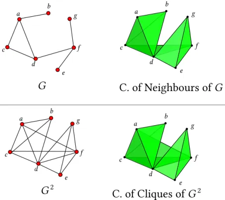
How to read figures. Each part of this thesis contains many examples illustrated

by figures where graphs and simplicial complexes were put beside. Graphs are drawn with red points as vertices, while vertices of simplicial complexes are black, and sim-plices of higher dimension are colored in green.

G

=({

a,b,c,d

}

,

{

ab,bc,ac,dc

})

Δ

=<

a,b,c

>

∪

<

c,d

>

d

c

a

b

d

c

Graphs

Definition 1(Graph). An (undirected, simple) graph𝐺 is an ordered pair𝐺 = (𝑉 , 𝐸)

where𝑉 is a set of vertices, and𝐸is a set of edges, which are 2-element subsets of𝑉.

So every edge is a couple of two distinct unordered vertices.

Definition 2. Let𝐺 = (𝑉 , 𝐸)be a graph.

• (Adjacent vertices) An adjacent vertex of𝑣 ∈ 𝑉 is a vertex that is connected to𝑣

by an edge.

• (Paths and Cycles) Let𝑣 , 𝑤 ∈ 𝑉. A path from𝑣 to𝑤 is a sequence of pairwise

adjacent vertices𝑣 𝑣1𝑣2⋯ 𝑣𝑛𝑤. The path is simple if no vertex is repeated in the

sequence. The path is a cycle if𝑣 = 𝑤. The path has length𝑘if it pass through𝑘

edges. The distance between𝑣and𝑤 is the minimum length of the paths from 𝑣to𝑤. If such a path does not exists, the distance is said to be infinite.

• (Connected graph)𝐺 is connected if for every couple𝑣 , 𝑤 ∈ 𝑉 exists a path from

𝑣to𝑤.

• (Isomorphism of graphs) Let𝐺 = (𝑉 , 𝐸)and𝐻 = (𝑊 , 𝐹 ) be two graphs. We say

that 𝐺 and 𝐻 are isomorphic if there is a bijection 𝜑 ∶ 𝑉 → 𝑊 such that: ({𝑣 , 𝑤 } ∈ 𝐸 ⇔ {𝜑(𝑣 ), 𝜑(𝑤 )} ∈ 𝐹 ).

• (Induced Graph) Let 𝑊 ⊂ 𝑉 and 𝐸(𝑊 ) = {{𝑖, 𝑗 } ∈ 𝐸 ∶ 𝑖, 𝑗 ∈ 𝑊 }. We define

𝐺 [𝑊 ] = (𝑊 , 𝐸(𝑊 ))the subgraph of𝐺induced by𝑊. Equivalently,𝐺 [𝑊 ]is the

subgraph formed from the vertices in 𝑊 and all of the edges in𝐸 connecting

pairs of vertices in𝑊.

• (Tree) A tree is an acyclic connected graph.

• (Complementary graph) The complementary graph of𝐺is:

𝐺𝐶 = (𝑉 , {{𝑥 , 𝑦 } ∶ 𝑥 , 𝑦 ∈ 𝑉 , 𝑥 ≠ 𝑦 and{𝑥 , 𝑦 } ∉ 𝐸}

Equivalently, 𝐺𝐶 is the graph whose vertices are the vertices of 𝐺 and whose

edges are the edges that are not present in𝐺.

• A set of vertices of a graph of cardinality𝑛will be denoted𝑉𝑛

• (Complete graph on𝑛 vertices) 𝐾𝑛 = (𝑉𝑛, 𝐸(𝐾𝑛)), is defined as follows: for every

𝑣1, 𝑣2 ∈ 𝑉𝑛 ⇒ {𝑣1, 𝑣2} ∈ 𝐸(𝐾𝑛)

• (Complete bipartite graph on𝑛and𝑚vertices)𝐾𝑛,𝑚 = (𝑉𝑛∪ 𝑉𝑚, 𝐸𝑛,𝑚), is defined as

follows: ⎧ ⎪ ⎪ ⎪ ⎪ ⎪ ⎨ ⎪ ⎪ ⎪ ⎪ ⎪ ⎩ 𝑉𝑛 ∩ 𝑉𝑚 = ∅, ∀ 𝑣1∈ 𝑉𝑛, 𝑣2∈ 𝑉𝑚 ⇒ {𝑣1, 𝑣2} ∈ 𝐸𝑛,𝑚, ∀ 𝑣1, 𝑣2∈ 𝑉𝑛 ⇒ {𝑣1, 𝑣2} ∉ 𝐸𝑛,𝑚, ∀ 𝑣1, 𝑣2∈ 𝑉𝑚 ⇒ {𝑣1, 𝑣2} ∉ 𝐸𝑛,𝑚

• (Complete𝑚-partite graph)𝐾_𝑛

1,𝑛2,…,𝑛𝑚 is a graph whose set of vertices can be

par-titioned in𝑚subsets of respective cardinality𝑛1, … , 𝑛𝑚, where an edge is present

if and only if its ends are in different subsets of the partition.

• (Chromatic number) The chromatic number 𝛾 (𝐺 ) of a graph 𝐺 is the smallest

number of colors needed to color the vertices of𝐺so that no two adjacent

ver-tices share the same color. We say that𝐺is𝑘-colorable for every𝑘 ≤ 𝛾 (𝐺 ).

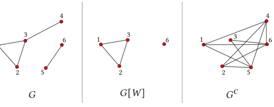
Example. The graph𝐺represented in fig. 1, along with𝐺𝐶, and𝐺 [𝑊 ], where𝑊 = {1, 2, 3, 6}: 𝐺 =({1, 2, 3, 4, 5, 6}, {{1, 2}, {2, 3}, {1, 3}, {3, 4}, {5, 6}}) 𝐺 [𝑊 ] =({1, 2, 3, 6}, {{1, 2}, {2, 3}, {1, 3}}) 𝐺𝐶 =({1, 2, 3, 4, 5, 6}, { {1, 4}, {1, 6}, {1, 5}, {2, 4}, {2, 5}, {2, 6}, {3, 5}, {5, 6}, {4, 5}, {4, 6} } )

Simplicial complexes

Definition 3(Abstract simplicial complex). A familyΔ of finite subsets of a set𝑉 is

anabstract simplicial complexif, for every𝜎 ∈ Δ, every subset𝜏 ⊂ 𝜎 also belongs toΔ

(inheritance property). We will call every set𝜎 ∈ Δof cardinality(𝑛 + 1)an𝑛-simplex,

1 2 3 4 5 6 G _{G [W]} GC 1 2 3 6 1 2 3 4 5 6

Figure 1: A simple graph 𝐺 on 6 vertices and 5 edges, along with the induced graph 𝐺 [𝑊 ]on the set of vertices𝑊 = {1, 2, 3, 6}, and the complementary graph𝐺𝐶.

Notation. We will indicate the power set of the set{𝑥₀, … , 𝑥_𝑛}as< 𝑥₀, … , 𝑥_𝑛 >. So,

if𝜎 is an𝑛-simplex on the vertices𝑥0, … , 𝑥𝑛, the simplicial complex made of𝜎 and all

its faces will beΔ =< 𝑥0, … , 𝑥𝑛 >.

Remark 4. I stick to the definition given by Jonsson in [15], including the emptyset

∅in every simplicial complex.

Definition 5 (Barycentric subdivision). The Barycentric Subdivision of a simplex Δ

is the simplicial complex sd(Δ)on a set 𝑉. 𝑉 is in bijection with the faces ofΔ and

very sequence 𝐹0, 𝐹1, … , 𝐹𝑛 of faces ofΔ, totally ordered by inclusion, is an𝑛-simplex

of sd(Δ), with vertices{𝑣0, … , 𝑣𝑛}. Each vertex𝑣𝑖 is called the barycenter of the face

𝐹𝑖.

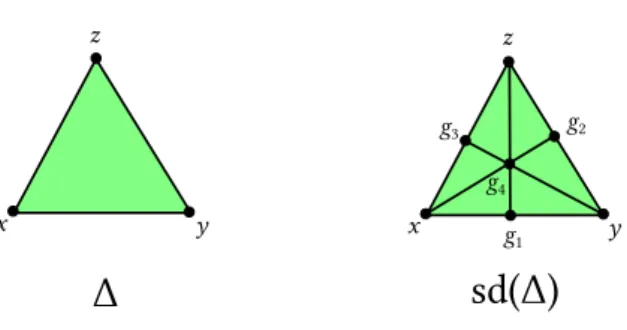
Example. The following simplicial complex (fig. 2) represent a 2-simplex and all its

faces: Δ = { ∅, {𝑥 }, {𝑦 }, {𝑧 }, {𝑥 , 𝑦 }, {𝑦 , 𝑧 }, {𝑥 , 𝑧 }, {𝑥 , 𝑦 , 𝑧 } } =< 𝑥 , 𝑦 , 𝑧 >

And this is its first barycentric subdivision: sd(Δ) = { ∅, {𝑥 }, {𝑦 }, {𝑧 }, {𝑔1}{𝑔2}, {𝑔3}, {𝑔4}, {𝑥 , 𝑔1}, {𝑔1, 𝑦 }, {𝑦 , 𝑔2}, {𝑔2, 𝑧 }, {𝑧 , 𝑔3}, {𝑔3, 𝑥 }, {𝑔1, 𝑔4}, {𝑔4, 𝑧 }, {𝑔2, 𝑔4}, {𝑔4, 𝑥 }, {𝑔3, 𝑔4}, {𝑔4, 𝑦 }, {𝑥 , 𝑔₁, 𝑔₄}, {𝑥 , 𝑔₃, 𝑔₄}, {𝑦 , 𝑔₁, 𝑔₄}, {𝑦 , 𝑔₃, 𝑔₄}, {𝑧 , 𝑔₁, 𝑔₄}, {𝑧 , 𝑔₂, 𝑔₄} } = < 𝑥 , 𝑔₁, 𝑔₄> ∪ < 𝑥 , 𝑔₃, 𝑔₄> ∪ < 𝑦 , 𝑔₁, 𝑔₄ > ∪ < 𝑦 , 𝑔₂, 𝑔₄> ∪ ∪ < 𝑧 , 𝑔₂, 𝑔₄> ∪ < 𝑧 , 𝑔₃, 𝑔₄ >

x y z x y z g3 g2 g1 g4

Δ

sd(

Δ

)

Figure 2: The simplicial complex described in the example and its first barycentric subdivision.

Definition 6(𝑘-skeleton of a simplicial complex). LetΔbe a simplicial complex and 𝑘 ∈_N∪{0}. The𝑘-skeleton ofΔis the simplicial complexΓ = {𝜎 ∈ Δ ∶ |𝜎 | < (𝑘 + 1)}.

For example the 1-skeleton of a simplicial complex Δ is the simplicial complex

containing all 0-simplices and 1-simplices inΔ.

Definition 7(Join). The join of two non-empty familiesΔandΓ(assumed to be defined

on disjoint ground sets) is the family:

Δ ∗ Γ = {𝜎 ∪ 𝜏 ∶ 𝜎 ∈ Δ, 𝜏 ∈ Γ}

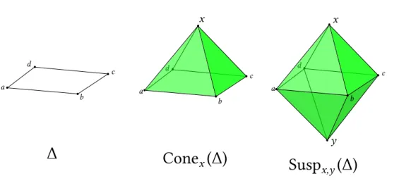
Definition 8 (Cones and Suspensions). The cone of a family Δ is the join with a

0-simplex:

Cone𝑥(Δ) = {∅, {𝑥 }} ∗ Δ

The suspension ofΔis the join with two 0-simplices:

Susp𝑥 ,𝑦(Δ) = {∅, {𝑥 }, {𝑦 }} ∗ Δ

Simplicial Homology

Homology is a standard in Algebraic Topology subject, that we will only consider in the simplicial case, although it can be described in more general settings (see for example [13],[22]). Moreover, we only consider homology on the fieldZ2 = Z/2Z, while it

could be defined also on an arbitrary group, or module over a ring. Our choice allows us not to require an orientation on simplices. In addition, homology groups will not show any torsion.

Definition 9(𝑛-chains). Let𝐾 be a simplicial complex. A simplicial𝑛-chain (𝑛 ∈ _Z)

is a formal sum of𝑛-simplices of𝐾: 𝑐 =

𝑘

∑

𝑖=1

d d

Δ

Cone

x

(

Δ

)

Susp

_x,y

(

Δ

)

x x y a d b c a b c a b c

Figure 3: The Cone and the Suspension of the simplicial complex Δ = {∅, {𝑎}, {𝑏}, {𝑐 }, {𝑑 }, {𝑎, 𝑏}, {𝑏, 𝑐 }, {𝑐 , 𝑑 }, {𝑑 , 𝑎}}

We can assume that every𝑛-simplex is present in each𝑛-chain: the formal sum does

not change adding any 𝑛-simplex with coefficient 𝛼𝑖 = 0. We define the sum of two

𝑛-chains𝑐1 = ∑ 𝛼𝑖𝜎𝑖, 𝑐2 = ∑ 𝛽𝑖𝜎𝑖 as: 𝑐1+ 𝑐2= ∑(𝛼𝑖 + 𝛽𝑖)𝜎𝑖.

The set of𝑛-chains, denotedC_𝑛orC_𝑛(𝐾 ), equipped with this operation of sum, is a

group where the neutral element is the null chain (that is the chain with every𝛼𝑖 = 0)

and the opposite of 𝑐 ∈ C𝑛 is𝑐 itself, since the coefficients sum up inZ2. The group

inherits the commutative property byZ2. Remark that the group of𝑛-chains is trivial

if𝑛is less than 0 or greater than the dimension of𝐾.

Definition 10(Boundaries). The boundary of an𝑛-simplex𝜎 = {𝑣0, … , 𝑣𝑛}is defined

as the chain of its(𝑛 − 1)-faces: 𝜕𝑛(𝜎 ) =

𝑛

∑

𝑖=0

{𝑣0, … , ̂𝑣𝑖, … , 𝑣𝑛}

where the hat means that the vertex was eliminated from the set:

{𝑣0, … , ̂𝑣𝑖, … , 𝑣𝑛} = {𝑣0, … , 𝑣𝑖−1, 𝑣𝑖+1, … , 𝑣𝑛}. Remark that𝜕𝑛(𝜎 ) ∈ C𝑛−1.

The𝑛-boundary of a simplicial complex is defined as the sum of boundaries of its 𝑛-simplices. This definition implies that𝜕_𝑛 ∶C_𝑛 →C_𝑛−1is a group homomorphism: if 𝑐1, 𝑐2 ∈C𝑛 then𝜕𝑛(𝑐1+ 𝑐2) = 𝜕𝑛(𝑐1) + 𝜕𝑛(𝑐2).

We have a sequence of abelian groups that we call achain complex: … 𝜕𝑛+2 ← ←←←←←←←←←←←←←←←←←←←←→C𝑛+1 𝜕𝑛+1 ← ←←←←←←←←←←←←←←←←←←←←→C𝑛 𝜕𝑛 ← ←←←←←←←←←←→ … 𝜕1 ← ←←←←←←←←←←→C0 𝜕0 ← ←←←←←←←←←←→ 0

Every𝑐 ∈ C𝑛 such that𝜕𝑛(𝑐 ) = 0is called an𝑛-cycle. We denote the set of𝑛-cycles by

Any𝑎 ∈ C𝑛 such𝜕𝑛+1(𝑏) = 𝑎for some𝑏 ∈C𝑛+1is called an𝑛-boundary. We denote

the set of𝑛-boundaries asB_𝑛.B_𝑛 ⊆C_𝑛 is the image of𝜕_𝑛+1and a subgroup ofC_𝑛.

Lemma 11(Homology lemma). 𝜕𝑛−1◦ 𝜕𝑛 = 0for every𝑛 ∈Z

Proof. For every simplex𝜎 = {𝑣0, … , 𝑣𝑛}we have:

𝜕𝑛−1(𝜕𝑛(𝜎 )) = 𝜕𝑛−1 ( 𝑛 ∑ 𝑖=0 {𝑣0, … , ̂𝑣𝑖, … , 𝑣𝑛} ) = 𝑛 ∑ 𝑖=0 𝜕𝑛−1({𝑣0, … , ̂𝑣𝑖, … , 𝑣𝑛}) = 𝑛 ∑ 𝑖=0( 𝑖−1 ∑ 𝑗 =0 {𝑣₀, … , ̂𝑣_𝑗, … , ̂𝑣_𝑖, … , 𝑣_𝑛} + 𝑛 ∑ 𝑗 =𝑖+1 {𝑣₀, … , ̂𝑣_𝑖, … , ̂𝑣_𝑖… , 𝑣_𝑛} )

In the last sum we have the same chains added twice, so the result is zero. Then, for linearity,𝜕_𝑛−1◦ 𝜕_𝑛 = 0holds for every simplicial complex.

From lemma 11 follows thatB𝑛 ⊂Z𝑛, because𝑏 ∈ B𝑛if𝑏 = 𝜕𝑛+1(𝑐 )for some𝑐 ∈C𝑛+1,

then𝜕𝑛(𝑏) = 𝜕𝑛(𝜕𝑛+1(𝑐 )) = 0. This remark allows us to give the next definition.

Definition 12. The 𝑛th simplicial homology group of a simplicial complex 𝐾 is the

quotient of abelian groups:

H𝑛(𝐾 ) =

Z𝑛(𝐾 )

/_B

𝑛(𝐾 )

All the sets we considered so far (C𝑛,Z𝑛,B𝑛,H𝑛) are groups, but also Z2-vector

spaces for every𝑛 ∈_Z. Thus the following dimensional equations holds: 𝜋 ∶Z𝑛 → Z𝑛/B𝑛 =H𝑛

⇒dim(Z_𝑛) =dim(ker(𝜋 )) +dim(Im(𝜋 )) =dim(B_𝑛) +dim(H_𝑛) 𝜕𝑛 ∶ C𝑛 → B𝑛−1

⇒dim(C𝑛) = dim(ker(𝜕𝑛)) +dim(Im(𝜕𝑛)) =dim(Z𝑛) +dim(B𝑛−1)

Definition 13. The𝑛thBetti number of a simplicial complex is the dimension of its𝑛th

homology group:

Simplicial compexes built from a

graph

Contents

1.1 Abstract . . . 15

1.2 Complex of Cliques . . . 17

1.3 Complex of Independent sets . . . 19

1.4 Complex of Neighbours . . . 21

1.5 Acyclic subsets . . . 25

1.5.1 Complex of induced acyclic subgraphs . . . 25

1.5.2 Complex of acyclic subsets of the edge set . . . 25

1.5.3 Complex of removable acyclic subgraphs . . . 26

1.6 Complex of enclaveless sets . . . 28

1.6.1 Enclaveless sets implementations . . . 29

1.1

Abstract

When considering a graph there are several methods to analyse its topology. It is possible to tackle this problem by building an abstract simplicial complex out of the graph, in order to use algebraic topology tools. The analysis of the resulting complex could provide topological insights about the original graph.

There are many well-studied methods to associate simplicial complexes out of a graph. In the literature the approach is twofold: on the one hand, there is the study of a family of simplicial complexes derived from graphs, where simplicial complexes

are studied with an interest in their own right (see [15], [4]). On the other hand, the study of a simplicial complex coming from a specific graph, in order to grasp additional information from the simplicial interpretation of the graph (see, e. g., [17], [21], [1]). This work mainly focuses on the latter approach: we want to find topological properties of the simplicial complex that could describe the original graph.

The following list provides a summary the methods described to build an abstract simplicial complex out of a graph. We also give here the references of various authors who use those methods to build simplicial complexes. In particular in [15] it is possible to find an encompassing description of several methods we do not consider in this work.

1. The complex of Cliques: consider every(𝑛 + 1)-clique of the graph as an

ab-stract𝑛-simplex (see for example: [15],[17], [21]);

2. The complex of Independent Sets:consider every(𝑛 + 1)-independent set of

the graph as an abstract𝑛-simplex (see for example: [15]);

3. The complex of neighbours: for every vertex 𝑣 ∈ 𝑉 consider the simplices

given by every subset of the set {𝑣 } ∪ {𝑤 ∈ 𝑉 ∶ 𝑤 is adjacent to𝑣 } (see for

example: [15] [16], [17]);

4. Complexes built from acyclic subsets:

• The complex of induced acyclic subsets: a set of vertices is a simplex if its induced graph is acyclic;

• The complex of acyclic subsets of the edge set: every edge is a 0-simplex and𝑛-simplices are given by(𝑛 + 1)edges forming an acyclic graph;

• The complex of removable acyclic subsets: simplices are given by non-disconnecting acyclic subsets of edges of a connected graph;

(Even though some references for these complexes can be found in [15], the at-tempts we made to explore these methods are due to professor Fabrizio Caselli’s suggestions.)

5. The complex of enclaveless sets:consider every enclaveless set of cardinality

(𝑛 + 1)as an𝑛-simplex (we could not find any reference for this method in the

1.2

Complex of Cliques

Definition 14(Clique). Let𝐺 = (𝑉 , 𝐸)be a simple graph. A set of vertices is a clique

in𝐺if the induced subgraph is complete. Formally, a subset𝐶 ⊂ 𝑉 is a clique of𝐺 if

for every pair𝑣 , 𝑤 ∈ 𝐶,𝑣 ≠ 𝑤, the edge{𝑣 , 𝑤 }is in𝐸.

Definition 15 (Complex of Cliques). The abstract simplicial complex of cliques of a

graph𝐺 = (𝑉 , 𝐸)is the abstract simplicial complex whose𝑛-simplices are the cliques

of𝐺 of cardinality(𝑛 + 1). This complex will be denoted asCl_𝐺.

Remark 16. Since every subset of a clique is still a clique,Cl𝐺 is well-defined.

This is the simplest way to build a simplicial complex out of a graph. In fact, the 1-skeleton of the complex is isomorphic to the graph, and where the graph is “dense” enough the complex is “filled” with simplices of higher dimension.

G

Δ

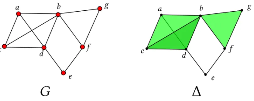
a b c _d e f g _{a b} c _d e f g

Figure 1.1: Example of a graph 𝐺 and its complex of cliques Δ =< 𝑎, 𝑏, 𝑐 , 𝑑 > ∪ < 𝑏, 𝑓 , 𝑔 > ∪ < 𝑑 , 𝑒 > ∪ < 𝑓 , 𝑒 >

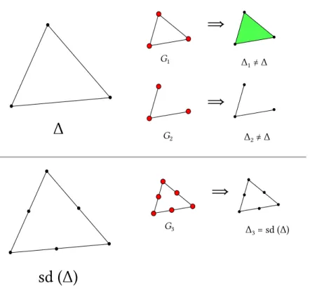
Observable simplicial complexes

Remark 17. Given a simplicial complexΔ, it is not possible to find a graph𝐺 = (𝑉 , 𝐸)

such thatCl𝐺 = Δ. As a counterexample see fig. 1.2.

The problem is that there is no graph𝐺 = (𝑉 , 𝐸)such thatCl𝐺 = 2 𝑉

⧵ {𝑉 }. However,

if we accept to subdivide the simplicial complex we want to be represented, we can find a suitable𝐺, as stated in the proposition 18.

Proposition 18. LetΔ be a simplicial complex and let sd(Δ) be its first barycentric

subdivison. If we consider the 1-skeleton of sd(Δ)as a graph𝐺 = (𝑉 , 𝐸), then we have

⇒

⇒

G1 G2 Δ₁ ≠ Δ Δ2 ≠ Δ

Δ

⇒

G3 _{Δ3 = sd (Δ)}

sd (

Δ

)

Figure 1.2: It is impossible to find a graph𝐺 such that its complex of cliques is the

simplicial complexΔ(boundary of the 2-simplex), but it is possible to find a graph such

that its complex of cliques is sd(Δ).

Proof. We show that sd(Δ)is both a subset and a superset ofCl𝐺.

𝜎 ∈sd(Δ) ⇒ 𝜎 ∈Cl𝐺:

this is straightforward, since every simplex in sd(Δ)is necessarily a clique in𝐺, thus a

simplex inCl𝐺.

𝜎 ∈Cl_𝐺 ⇒ 𝜎 ∈sd(Δ):

𝜎 ∈Cl𝐺 means that𝜎 is a clique of the 1-skeleton of sd(Δ).

By induction on𝑛 = |𝜎 |we are going to show:

𝑃 (𝑛) ∶for every clique𝜎in𝐺, its vertices are barycenters of simplices forming a chain of faces of the same simplex.

This will prove the claim, since𝑃 (𝑛)is precisely the definition of a simplex𝜎 in sd(Δ).

For𝑛 = 1,𝑃 (1)is trivial.

𝑃 (𝑛 − 1) ⇒ 𝑃 (𝑛): in a barycentric subdivision every barycenter belongs to a simplex

of dimension different from the adjacent barycenters. For every clique𝜎 we consider

clique). Thus the (𝑛 − 1) adjacent vertices are barycenters of faces of 𝜏, and, by the

induction hypothesis, they all belong to the same face. This proves𝑃 (𝑛).

Homology of the complex of cliques

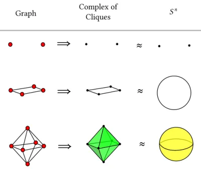
Proposition 19(Suspensions). Let 𝐺 = (𝑉 , 𝐸)be a graph, let Cl𝐺 be its complex of

cliques, and𝑥 , 𝑦 ∉ 𝑉. Let CSusp(𝐺 )be the graph:

CSusp(𝐺 ) ∶= (𝑉 ∪ {𝑥 , 𝑦 }, 𝐸 ∪ { {𝑣 , 𝑥 }, {𝑣 , 𝑦 } ∶ 𝑣 ∈ 𝑉 } )

Then the complex of cliques of CSusp(𝐺 )is Susp

𝑥 ,𝑦(Cl𝐺).

Proof. By definition of suspension:𝜎 ∈Susp

𝑥 ,𝑦(Cl𝐺)if and only if one of the following

conditions holds: 1. 𝜎 ∈Cl𝐺;

2. (𝜎 ⧵ 𝑥 ) ∈Cl𝐺;

3. (𝜎 ⧵ 𝑦 ) ∈Cl𝐺.

In each of the three cases, the definition of CSusp guarantees that 𝜎 is a clique in

CSusp(𝐺 ). In fact every subgraph of 𝐺 is still a subgraph of CSusp(𝐺 ), thus the first

case is proved. As for the second and the third case: consider(𝜎 ⧵ 𝑥 ) ∈ Cl𝐺, then, by

construction, each element of the clique (𝜎 ⧵ 𝑥 ) is connected to the vertex𝑥 in the

graph CSusp(𝐺 ). So𝜎 is a clique in CSusp(𝐺 ).

Remark 20. By definition CSusp(𝐺 )is obtained from𝐺by adding two vertices

com-pletely connected to the other vertices of 𝐺, but not with each other. If we iterate𝑛

times the suspension of the graph𝐺 = ({𝑥 , 𝑦 }, ∅)we obtain graphs that are represented

by a simplicial complex of cliques whose euclidean embedding is homeomorphic to the sphere𝑆𝑛(see fig. 1.3). Thus the reduced homology groups of that simplicial complex

are all trivial, except the𝑛-th.

1.3

Complex of Independent sets

Definition 21(Independent set). Let𝐺 = (𝑉 , 𝐸)be a simple graph. A set of vertices is

an independent set in𝐺if the induced subgraph does not contain any edge. Formally,

a subset𝐼 ⊂ 𝑉 is an independent set of𝐺, if every pair𝑣 , 𝑤 ∈ 𝐼 is such that{𝑣 , 𝑤 } ∉ 𝐸.

Definition 22(Complex of Independent sets). The abstract simplicial complex of

in-dependent sets of a graph𝐺 = (𝑉 , 𝐸)is the one whose𝑛-simplices are the independent

⇒

⇒

⇒

≈

≈

≈

Graph Complex of_Cliques S n

Figure 1.3: The first two suspensions of the graph𝐺 = ({𝑥 , 𝑦 }, ∅)

Lemma 23(Complex of cliques is the complex of independent sets of the

complemen-tary). Let𝐺 = (𝑉 , 𝐸)be a graph. ThenCl_𝐺 =I_𝐺𝐶.

Proof. To prove the lemma it suffices to remark that, by definition of complementary

graph, a clique in𝐺is an independent set of𝐺𝐶.

Remark 24.lemma 23 implies that everything we previously stated about the complex

of cliques holds also for the complex of independent sets of the complementary graph. By the way we will briefly recall those results in the following propositions.

Proposition 25. Let Δ be a simplicial complex and let sd(Δ)be its first barycentric

subdivison. If we consider the 1-skeleton of sd(Δ)as a graph 𝐺 = (𝑉 , 𝐸), thenI_𝐺𝐶 =

sd(Δ).

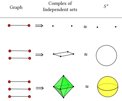
Proposition 26 (Suspensions). Let 𝐺 = (𝑉 , 𝐸) be a graph, and let 𝑥 , 𝑦 ∉ 𝑉. Let

ISusp(𝐺 )be the graph:

ISusp(𝐺 ) ∶= (𝑉 ∪ {𝑥 , 𝑦 }, 𝐸 ∪ { {𝑥 , 𝑦 } } )

Then the complex of independent sets of ISusp(𝐺 )is Susp

𝑥 ,𝑦(I𝐺).

Remark 27. By definition ISusp(𝐺 )ISusp(𝐺 ) is𝐺obtained with the addition of two

suspension of the graph𝐺 = ({𝑥 , 𝑦 }, {𝑥 , 𝑦 })we obtain graphs that are represented by

a simplicial complex of independent sets that is homeomorphic to the sphere𝑆𝑛 (see

fig. 1.4. Thus the reduced homology groups of that simplicial complex are all trivial, except the𝑛-th.

⇒

⇒

⇒

≈

≈

≈

Graph _{Independent sets}Complex of S n

Figure 1.4: The first two suspensions of the graph𝐺 = ({𝑥 , 𝑦 }, {𝑥 , 𝑦 })

1.4

Complex of Neighbours

Definition 28 (neighbours). Let 𝐺 = (𝑉 , 𝐸) be a graph and let 𝑣 ∈ 𝑉. The set of

neighbours of𝑣is

𝑁 (𝑣 ) = {

𝑤 ∈ 𝑉 ∶ {𝑣 , 𝑤 } ∈ 𝐸 }

Definition 29(Complex of neighbours). Simplices of the abstract simplicial complex

of neighbours of a graph𝐺 = (𝑉 , 𝐸)are all the subsets of{𝑣 } ∪ 𝑁 (𝑣 ), for every𝑣 ∈ 𝑉.

This complex will be denotedNb𝐺.

Remark 30. The inheritance property is included in the definition, so the simplicial

complex is well-defined.

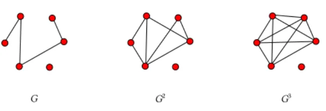
We have various obvious straightforward relations between thedegree of the

G G2 _G3

Figure 1.5: An example of graph and its powergraphs.

is equal to the greatest dimension of the simplices of the complex of neighbours. More-over if𝐺 is a regular graph (every vertex has the same degree)Nb𝐺 is a homogeneous

simplicial complex.

Observable simplicial complexes

Definition 31(Power graph). Let 𝐺 = (𝑉 , 𝐸). For𝑘 ∈ _Nwe define the power graph 𝐺𝑘 as the graph that has𝑉 as a set of vertices and where two vertices are adjacent if

their distance in𝐺is at most𝑘.

Lemma 32 (Complex of neighbours is subcomplex of the complex of cliques of the

power graph). Let𝐺 = (𝑉 , 𝐸)be a graph. ThenNb𝐺 ⊂Cl𝐺2.

Proof. Let 𝜎 ∈ Nb𝐺, then there is a vertex 𝑣 ∈ 𝜎 such that𝜎 ⊆ {𝑣 } ∪ 𝑁 (𝑣 ). Thus the

distance among the vertices of𝜎 is at most 2 (they all have a common neighbour) and

this implies that the set of vertices𝜎 is a clique in𝐺2.

Remark 33. The converse ( Cl𝐺2 ⊆ Nb

𝐺) is not true. For example fig. 1.6 is a

coun-terexample.

Remark 34. Not all simplicial complexes are observable. For example there is not

such a graph whose simplicial complex is an empty triangle: it is sufficient to observe that if the graph has maximum degree bigger than 1, then we have at least a 2-simplex. Moreover the first barycentric subdivision does not provide the homeomorphism of the bodies (as the complex of cliques provided), but probably we could have homotopic equivalence (see fig. 1.7).

Homology and Homotopy of the complex of neighbours

The complex of neighbours, as stated in lemma 32, is a super-complex of the complex of cliques of𝐺, and a sub-complex of the complex of cliques of𝐺2. This fact prevents

G

C. of Neighbours of

G

a b c d e f g a b c d e f g

G

2 a b c d e f g _a b c d e f g

C. of Cliques of

G

2

Figure 1.6: Example of the complex of neighbours of a graph𝐺: Nb𝐺 =< 𝑎, 𝑏, 𝑐 , 𝑑 >

∪ < 𝑑 , 𝑒, 𝑓 , 𝑔 > ∪ < 𝑐 , 𝑑 , 𝑓 >. Moreover we have: Cl𝐺2 =< 𝑎, 𝑏, 𝑐 , 𝑑 > ∪ < 𝑑 , 𝑒, 𝑓 , 𝑔 > ∪ < 𝑎, 𝑐 , 𝑑 , 𝑓 >, soNb_𝐺 ⊊Cl_𝐺2

≈

≈

⇒

⇒

Figure 1.7: Refining a triangle does not give a complex of neighbours PL-equivalent to an empty triangle, but at least provide homotopical equivalence

The main preserved information about the original graph is the connectedness. To each connected component of the graph corresponds a connected component of the simplicial complex, and connected components of a graph are preserved via the power graph.

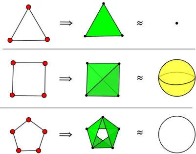
Definition 35(Chordless cycle). A chordless cycle in a graph𝐺 is a cycle such that

no two vertices of the cycle are connected by an edge that does not itself belong to the cycle.

Remark 36(𝑛-cycles). Let𝐺 = (𝑉 , 𝐸)be a chordless cycle on𝑛 vertices and letNb𝐺

be its complex of neighbours. • if𝑛 = 3, thenNb𝐺 = 2

𝑉 is a 2-simplex.

• if𝑛 = 4, thenNb𝐺 = 2 𝑉

⧵ 𝑉. That is: Nb𝐺 is the complex containing the faces

of a 3-simplex but not the 3-simplex itself (i.e. is an empty tetrahedron). So it is simply connected and has the homotopy type of the 2-sphere𝑆2.

• if 𝑛 ≥ 5, Nb𝐺 is homotopically equivalent to 𝑆

1. [ In particular is not simply

connected, and a representant of the fundamental group is the loop given by the simplexes forming the cycle in𝐺.]

⇒

⇒

≈

⇒

≈

≈

Figure 1.8: Illustration of the graphs and the simplicial complexes of neighbours con-sidered in remark 36

We state now a result form Lov´asz [16], which relates the connectedness of the complex of neighbours with the chromatic number of the original graph. A topological

space𝑇is called𝑛-connectedif each continuous mapping of the surface𝑆𝑟of the(𝑟 + 1)

-dimensional ball into𝑇 extends continuously to the whole ball, for𝑟 ∈ {0, 1, … , 𝑛}.

Theorem 37. If the complex of neighbours of𝐺 is(𝑘 + 2)-connected, then 𝐺 is not 𝑘-colorable.

1.5

Acyclic subsets

We acknowledge professor Fabrizio Caselli1_{, for his valuable contribution to this}

sec-tion, in which we describe three methods to build simplicial complexes from acyclic subgraphs.

1.5.1

Complex of induced acyclic subgraphs

Definition 38. Let 𝐺 = (𝑉 , 𝐸)be a simple graph. The simplicial complex of induced

acyclic subgraphs of𝐺is the simplicial complexΔsuch that𝜎 ⊂ 𝑉 is a simplex inΔif

the induced subgraph𝐺 [𝜎 ]is acyclic.

Remark 39. The simplicial complex is well-defined since if𝜏 ⊂ 𝜎 then𝐺 [𝜏 ] ⊂ 𝐺 [𝜎 ],

and every subgraph of an acyclic graph is still acyclic.

The 1-skeleton of the complex of induced acyclic subgraphs of every graph 𝐺 = (𝑉 , 𝐸)is always isomorphic to the complete graph on|𝑉 |vertices. In fact, let𝑥 , 𝑦 ∈ 𝑉.

Then𝐺 [𝑥 , 𝑦 ]is acyclic in any case: both if𝐺 [𝑥 , 𝑦 ] = ({𝑥 , 𝑦 }, ∅), either or if𝐺 [𝑥 , 𝑦 ] = ({𝑥 , 𝑦 }, {𝑥 , 𝑦 }).

Moreover this complex preserves very little topological information of the orig-inal graph: every acyclic induced subgraph on (𝑛 + 1)-vertices is represented by an 𝑛-simplex, regardless of the structure of the subgraph (see fig. 1.9).

1.5.2

Complex of acyclic subsets of the edge set

Definition 40. Let 𝐺 = (𝑉 , 𝐸) be a graph and let 𝜑 ∶ 𝐼 → 𝐸 be a bijection. The

simplicial complex of acyclic subsets of the edge set is the simplicial complex on 𝐼

such that𝜎 ⊂ 𝐼 is a simplex if𝜑(𝜎 )is an acyclic subgraph of𝐺.

Remark 41. In the simplicial complex of acyclic subsets of the edge set 0-simplices

are represented by the edges of the graph, while in the previous methods 0-simplices were represented by the vertices of the graph. The complex is well-defined since every subgraph of an acyclic graph is still acyclic.

⇒

⇒

⇒

⇒

Figure 1.9: Every acyclic graph on 5 vertices is represented (as a complex of induced acyclic subgraphs) by a simplicial complex containing a 4-simplex and all its faces.

We lose much topological information about the original graph: every acyclic sub-graph on𝑛 + 1edges is represented by an 𝑛-simplex,while the pieces of information

about inner structure, connected components, degree of the vertices of the acyclic sub-graph is lost (see fig. 1.10).

Remark 42. A special case of subcomplex of the acyclic subsets of the edge set is the

well studiedmatching complex (see [8] and [3]), where the vertex set of this complex

is the set of edges of𝐺and its faces are sets of edges of𝐺 with no two edges meeting

at a vertex.

1.5.3

Complex of removable acyclic subgraphs

Definition 43. Let𝐺 = (𝑉 , 𝐸)be a connected graph and let𝜑 ∶ 𝐼 → 𝐸 be a bijection.

The simplicial complex of removable acyclic subgraphs is the simplicial complex on𝐼

such that𝜎 ⊂ 𝐼 is a simplex if𝜑(𝜎 )is an acyclic subgraph of𝐺 and𝐺′= (𝑉 , 𝐸 ⧵ 𝜑(𝜎 ))

is still connected.

Remark 44. This graph is well-defined because, as usual, a subgraph of an acyclic

graph is still acyclic, and if we remove a smaller number of edges the graph is still connected.

As in remark 39 and remark 41 the structure of the removed subgraph is not sig-nificant.𝑛-simplices are generated by sets of(𝑛 + 1)edges, regardlessly of the

a b c d a b c d a b c d a b c d

⇒

⇒

⇒

Figure 1.10: Every acyclic graph on 4 edges is represented (as a complex of acyclic subgraphs of the edge set) by a simplicial complex containing a 3-simplex and all its faces.

Proposition 45. In the complete graph on 𝑛 vertices𝐾_𝑛, the complex of removable

acyclic subgraphs is homogeneous of dimension(𝑛 − 2)and the simplices of maximal

dimension are𝑛𝑛−2− 𝑛.

Proof. The dimension of the complex comes from two standard graph theory theorems

about trees and spanning trees: every tree has exactly as much vertices as the number of edges minus one, and every graph is connected if and only if it has a spanning tree (see [6, theorem 4.3, theorem 4.6]).

As for the number of simplices: in𝐾𝑛 there are𝑛

𝑛−2spanning trees (Cayley’s

for-mula, see [6, theorem 4.8]). We are now going to show that, if we remove from𝐾𝑛 the

edges of one of these trees, the resulting graph is disconnected only in𝑛 cases. This

will prove that the simplices of maximal dimension are𝑛𝑛−2− 𝑛.

In order to disconnect𝐾𝑛it is necessary to divide at least one vertex from the others,

that is: we have to remove each of the𝑛 − 1edges starting from that vertex.

Another possibility, for example, is to disconnect a couple of vertices from the others: this can be achieved removing 𝑛 − 2edges from the first vertex and 𝑛 − 2

from the second vertex, while the edge connecting the two vertices can be preserved. Thus we removed2(𝑛 − 2)edges overall.

Similarly, to disconnect a clique of𝑘vertices from the rest of the graph we have to

remove at least𝑘 (𝑛 − 𝑘 )edges.

Moreover, those edges must belong to an acyclic subgraph of𝐾𝑛, so their number

must be smaller than𝑛 − 1.

fol-lowing constraint on the number of the removed edges:

𝑘 (𝑛 − 𝑘 ) ≤ 𝑛 − 1 𝑛 ∈_N, 𝑛 ≥ 2 −𝑘2+ 𝑘 𝑛 − 𝑛 + 1 ≤ 0

This second degree inequality is solved for𝑘 ≤ 1 or𝑘 ≥ 𝑛 − 1. Both the acceptable

solutions𝑘 = 1and 𝑘 = 𝑛 − 1mean are separating one of the 𝑛 vertices from 𝐾_𝑛 by

removing its𝑛 − 1 incident edges. So there are only 𝑛 spanning trees whose edges

disconnect𝐾𝑛.

1.6

Complex of enclaveless sets

We did not find any reference in the literature that used this method to build simpli-cial complexes out of a graph. The definition of enclaveless set and further results in domination in graphs can be found in[14].

Definition 46(Enclaves and Enclaveless sets). Let𝐺 = (𝑉 , 𝐸)be a simple graph. For 𝑆 ⊂ 𝑉 a vertex𝑣 ∈ 𝑆 is an enclave if𝑁 (𝑣 ) ⊂ 𝑆. A set is said to be enclaveless if it does

not contain any enclaves.

Definition 47(Dominating set). Let𝐺 = (𝑉 , 𝐸)be a simple graph. A set of vertices𝐷

is dominating in𝐺if for every𝑣 ∈ 𝑉,𝑣 ∈ 𝐷or exist𝑤 ∈ 𝐷such that{𝑣 , 𝑤 } ∈ 𝐸. That

is: a set of vertices𝐷is dominating if every vertex in𝑉 is either in𝐷or adjacent to a

vertex in𝐷.

Remark 48. It is possible to characterize an enclaveless set as complementary of a

dominating set. In fact, if𝐷 is a dominating set, then every 𝑣 ∈ 𝑉 ⧵ 𝐷 adjacent to

a vertex in𝐷, so𝑁 (𝑣 ) is not a subset of𝑉 ⧵ 𝐷. Thus𝑉 ⧵ 𝐷is enclaveless for every

dominating set𝐷. Vice versa, if 𝑆 ⊂ 𝑉 is enclaveless, then every 𝑣 ∈ 𝑉 is either in 𝑉 ⧵ 𝑆or adjacent to it, because𝑁 (𝑣 )is not a subset of𝑆.

Definition 49 (Complex of enclaveless sets). The abstract simplicial complex of

en-claveless sets of a graph𝐺 = (𝑉 , 𝐸)is the one whose 𝑛-simplices are the enclaveless

sets of𝐺of cardinality(𝑛 + 1). We will denote this complex withEl_𝐺.

Remark 50. This complex is well defined. The inheritance property comes from the

fact that every superset of a dominating set is still a dominating set, thus a subset of an enclaveless set is still an enclaveless set.

Remark 51. There are many restrictions when we try to find a specific graph to build

a given simplicial complex. For example it is not possible to build a simplicial complex of enclaveless sets made by an 𝑛-simplex alone. Every time we have an 𝑛-simplex,

there is always a further 0-simplex in the complex, and this is due to the topological structure of a graph containing an enclaveless set of cardinality𝑛 + 1(see fig. 1.11).

⇒

Figure 1.11: On the left, the smallest graph with an enclaveless set of cardinality 6. On the left, its complex of enclaveless sets, made of a 5-simplex and a 0-simplex. In general, the smallest graph with an enclaveless set of cardinality 𝑛 has the same

structure: acyclic on𝑛 + 1vertices with a vertex of degree𝑛. Analogously its complex

of enclaveless sets is composed by an 𝑛-simplex (generated by the enclaveless set of

vertices of degree 1) and a 0-simplex (generated by the vertex of degree𝑛).

Homology of the complex of enclaveless sets

Proposition 52. The body of the geometric complexEl𝐾𝑛 is homeomorphic to𝑆

𝑛−2.

Proof. Minimal dominating sets of𝐾𝑛are the singletons, thus maximal enclaveless sets

of𝐾𝑛are subsets of vertices of cardinality(𝑛 − 1). So, in the complex of enclaveless sets

there are all the(𝑛 − 2)-simplices on𝑛vertices, and this is the geometric representation

of the boundary of an(𝑛 − 1)-simplex, and the body of this boundary is homeomorphic

to𝑆𝑛−2.

Proposition 53 (Suspensions). Let 𝐺 = (𝑉 , 𝐸) be a graph, and let 𝑥 , 𝑦 ∉ 𝑉. Let

ESusp(𝐺 )be the graph:

ESusp(𝐺 ) ∶= (𝑉 ∪ {𝑥 , 𝑦 }, 𝐸 ∪ { {𝑥 , 𝑦 } } )

Then the complex of enclaveless sets of ESusp(𝐺 )is Susp

𝑥 ,𝑦(El𝐺).

Remark 54. The definition of the graph ESusp(𝐺 )and ISusp(𝐺 )(see proposition 26) is

the same: the addition of two vertices connected with each other only. As in the case of the complex of independent sets, if we iterate𝑛times the suspension of the graph 𝐺 = ({𝑥 , 𝑦 }, {𝑥 , 𝑦 }) we obtain graphs that are represented by a simplicial complex

of independent sets that is homeomorphic to the sphere 𝑆𝑛 (the figure is identical to

fig. 1.4). Thus the reduced homology groups of that simplicial complex are all trivial, except the𝑛-th.

1.6.1

Enclaveless sets implementations

Looking for minimal dominating sets. We adapted the method designed to find

We define a symbolic way to refer to the subsets of the power set of𝑉. Let𝑣 , 𝑤 ∈ 𝑉,

then𝑣 + 𝑤is the set{{𝑣 }, {𝑤 }}and𝑣 ⋅ 𝑤is the set{{𝑣 , 𝑤 }}. These are logic operations:

we define the sum of two vertices to be “the first vertex either or the second vertex”

and the product of vertices to be “the first vertex and the second”. Those definitions

are generalizable to represent elements of the power set2𝑉 (products) and subsets of

the power set (additions of products). Using the distributive and associative properties we can exploit symbolic computations to manipulate the sets. It is possible to find all the minimal dominating sets of a graph𝐺following this procedure:

S =∅ for𝑣 ∈ 𝑉 do Nv ={{v}} for𝑤 ∈ 𝑁 (𝑣 )do Nv = Nv + w end S = S⋅Nv end

The main idea is that in every dominating set𝐷, every vertex of𝑉 must be either

in𝐷or at least have a neighbour contained in𝐷. So in the end we have: 2𝑉 ⊃ 𝑆 = ∏ 𝑣 ∈𝑉( 𝑣 + ∑ 𝑤 ∈𝑁 (𝑣 ) 𝑤 )

Once performed all the calculations, each product of vertices is a minimal dominating set.

Simplifications. There are a couple useful simplifications for the computation:

1. duplicates of every vertex that appears more than once in a product are remov-able (e.g.:𝑣 𝑤 𝑥 𝑣becomes𝑣 𝑤 𝑥).

2. if in a sum there are a couple of addends such that one is contained in the other, then the bigger addend is removable (e.g.𝑣 𝑤 𝑥 + 𝑣 𝑤 𝑥 𝑦 becomes𝑣 𝑤 𝑥).

3. let𝑝𝑖be products of vertices and𝑣𝑘be vertices. Then we can simplify the product

(𝑝₁+ ⋯ + 𝑝_𝑠)(𝑣₁+ ⋯ + 𝑣_𝑟). Let𝑝′

1, … , 𝑝 ′

ℎbe the products containing at least one of

the vertices𝑣1, … , 𝑣𝑟 and let𝑝 ′′ 1, … , 𝑝

′′

𝑘 be the products not containing any of the

vertices𝑣1, … , 𝑣𝑟. Then the product can be simplified in:

𝑝′ 1+ ⋯ + 𝑝 ′ ℎ+ (𝑝 ′′ 1 + ⋯ + 𝑝 ′′ 𝑘)(𝑣1+ ⋯ + 𝑣𝑟)

a

b c

d e

Figure 1.12: Example of a graph. The first step in the computation of minimal domi-nating sets for the graph above is the following:(𝑎 + 𝑏 + 𝑑 + 𝑒)(𝑏 + 𝑎 + 𝑐 )(𝑐 + 𝑏 + 𝑑 )(𝑑 + 𝑐 + 𝑎 + 𝑒)(𝑒 + 𝑎 + 𝑑 ).

Implementation. We tried to implement this strategy using the following idea:

ev-ery vertex is associated to a prime number and then computations are made with ar-rays: every element of the array is an addend of the sum and every element is a product of prime numbers. This way simplifications are easily performed: for simplification 1 it suffices to reduce every element of the array to a product of primes raised to the first power; for simplification 2, if an element of the array divides the other, then the divisible element is deleted (see appendix).

This solution is an elegant one, but the evidence shows that numbers grow steadily while the number of vertices grows and computations becomes challenging and the elaboration time slows down. So it is advisable to find another implementation strat-egy.

Graph persistence

Contents

2.1 Persistent homology: a brief introduction . . . 33 2.2 Persistent homologic properties for simplicial complexes from

a graph . . . 36 2.2.1 Case study: edge filtrations on𝐾₄ . . . 37

2.2.2 Filtration on edge-induced subgraphs: a simple example . . 48 2.2.3 Complexes from acyclic subsets and persistent homology . 48 2.3 Other Persistent properties: blocks and edge-blocks . . . 51 2.3.1 The persistent block number . . . 52 2.3.2 The persistent edge-block number . . . 53

2.1

Persistent homology: a brief introduction

Persistent homology is a useful method for computing topological features of a space. It was introduced by Patrizio Frosini and collaborators under the name of Size Theory [12] and used for shape recognition. This theory was also independently developed by Edelsbrunner et al. [9]. We consider only the case of persitent homology on simplicial complexes, but the general setting of the theory refers to topological spaces.

Let 𝐾 be a finite simplicial complex. We want to define a nested sequence of

in-creasing subcomplexes of 𝐾 called a filtration. So, let𝑓 ∶ 𝐾 → _R be a real valued

function such that 𝑓 is non-decreasing on increasing sequences of faces. That is: if 𝜎 , 𝜏 ∈ 𝐾 and𝜎 ⊂ 𝜏, then𝑓 (𝜎 ) ≤ 𝑓 (𝜏 ).

For every 𝑎 ∈ _R the sublevel set 𝐾 (𝑎) = 𝑓−1((−∞, 𝑎])is a subcomplex of 𝐾. The

hypothesis on𝑓 ensure that the ordering of the simplices provided by the values of𝑓

induces afiltration, that is an ordering on the sublevel complexes: ∅ = 𝐾0⊊ 𝐾1⊊ ⋯ ⊊ 𝐾𝑝 = 𝐾

Where𝐾𝑖 = 𝐾 (𝛼𝑖)and𝛼𝑖 ∈ [𝑎𝑖, 𝑎𝑖+1)for some𝑎𝑖 ∈R.

For every couple of 𝑖, 𝑗 such that 0 ≤ 𝑖 ≤ 𝑗 ≤ 𝑝, the inclusion 𝐾_𝑖 ↪ 𝐾_𝑗 induces a

homomorphism on the simplicial homology groups for each dimension𝑛: 𝑓𝑖,𝑗

𝑛 ∶H𝑛(𝐾𝑖) →H𝑛(𝐾𝑗)

For every 𝑛 ∈ {0, … , 𝑝} the 𝑛th persistent homology groups are the images of these

homomorphisms and the𝑛thpersistent Betti number are the ranks of those groups: 𝛽𝑖,𝑗

𝑛 =dim(Im𝑓 𝑖,𝑗 𝑛 )

Persistent Betti numbers count how many homology classes of dimension 𝑛 survive

the passage from𝐾_𝑖 to𝐾_𝑗. We say that a homology class 𝛼 ∈ H_𝑛(𝐾_𝑖)is born entering

in𝐾𝑖 if𝛼 does not come from a previous subcomplex, that is𝛼 ∉ Im𝑓 𝑖−1,𝑖

𝑛 . Similarly, if

𝛼 is born in 𝐾𝑖, itdies entering 𝐾𝑗 if the image of the map induced by𝐾𝑖−1 ⊂ 𝐾𝑗 −1 does

not contain the image of𝛼 but the image of the map induced by𝐾_𝑖−1⊂ 𝐾_𝑗 does. In this

case thepersistenceof𝛼 is𝑗 − 𝑖.

We can draw thepersistence diagramwhere we represent the points(𝑖, 𝑗 )where𝑖is

the birth of an homological class and𝑗is its death. If the class does not die we represent

a vertical line called cornerline, starting from the diagonal in correspondence of the

moment of its birth. In the diagram we usually draw the diagonal of the first and third quadrant.

This pairing of homology classes generalizes the pairing that Edelsbrunner calls “the elder rule”. The reason for this name is easily understood in the study of persis-tence for single variable functions𝑔 ∶_R→_R. When a new component is introduced

(a local minimum is found) in 𝑔−1(−∞, 𝑡 ] we say that the local minimum represent

the component (birth of the component at time𝑡). When passing a local maximum

and merging two components, we pair the maximum with the “younger” of two local minima that represent the two components, and the other minimum is now the rep-resentative of the component resulting from the merger [9]. This is the same strategy we will use to define other persistent properties of a graph in section 2.3.

Example. We show now a simple example of a simplicial complex and its

Let the filtration be the following sequence of nested simplicial complexes (see fig. 2.1): 𝐾0= ∅ 𝐾1 = {{𝑎, 𝑏}, {𝑎}, {𝑏}, ∅} 𝐾2 = {{𝑐 , 𝑑 }, {𝑐 }, {𝑑 }, {𝑎, 𝑏}, {𝑎}, {𝑏}, ∅} 𝐾₃ = {{𝑒, 𝑓 }, {𝑒}, {𝑓 }, {𝑐 , 𝑑 }, {𝑐 }, {𝑑 }, {𝑎, 𝑏}, {𝑎}, {𝑏}, ∅} 𝐾₄ = {{𝑎, 𝑏, 𝑐 }, {𝑎, 𝑐 }, {𝑏, 𝑐 }, {𝑒, 𝑓 }, {𝑒}, {𝑓 }, {𝑐 , 𝑑 }, {𝑐 }, {𝑑 }, {𝑎, 𝑏}, {𝑎}, {𝑏}, ∅} 𝐾5 = {{𝑎, 𝑐 , 𝑑 }, {𝑎, 𝑑 , 𝑓 }, {𝑓 , 𝑑 , 𝑐 }, {𝑎, 𝑑 }, {𝑎, 𝑓 }, {𝑓 , 𝑑 }, {𝑑 , 𝑒}, {𝑎, 𝑏, 𝑐 }, {𝑎, 𝑐 }, {𝑏, 𝑐 }, {𝑒, 𝑓 }, {𝑒}, {𝑓 }, {𝑐 , 𝑑 }, {𝑐 }, {𝑑 }, {𝑎, 𝑏}, {𝑎}, {𝑏}, ∅}

This example shows how to build a persistence diagram according to the definition above. 0 1 2 3 4 5 1 2 3 4 5 "death" of {a,b} ∞

birth of {birth of {a,b} c,d} birth of {e,f } death of {c,d} death of {e,f } 0 1 2 3 4 5 1 2 3 4 5 ∞ 0 1 2 2 3

⊂

⊂

⊂

⊂

⊂

K

₅ a b c d e f

K

₀ a

∅

a b c d e f

K

1 a b c d e f

K

2 a b c d e f

K

3 a b c d e f a

K

4 b c d e f

Figure 2.1: Example of a filtration (on top), its zero-persistence diagram (on the left), and the persistent betti number function (on the right)

2.2

Persistent homologic properties for simplicial

com-plexes from a graph

Definition 55. Aweighted graph𝐺 = (𝑉 , 𝐸, 𝑤 )is a graph𝐺 = (𝑉 , 𝐸)where theweight

function 𝑤 is a bijection 𝑤 ∶ 𝐸 → {1, 2, … , |𝐸|}. On 𝐺 = (𝑉 , 𝐸, 𝑤 ) we define the

subgraph𝐺_𝑖 = (𝑉 , 𝑤−1({1, 2, … , 𝑖}).

Ourfiltrationwill be the sequence of complexes associated to each𝐺𝑖 (see for

ex-ample fig. 2.2)

This setting allows us to study the persistence of the simplicial complexes described in chapter 1 (built from the various stages of the filtration of the edges).

⇒

⇒

⇒

1 2 3 4 6 7 8 9 5 G=(V,E,w) 1 2 3 4 G4 1 2 3 4 6 5 G7 1 2 3 4 6 7 8 9 5 G9 7

Figure 2.2: The weighted graph𝐺 = (𝑉 , 𝐸, 𝑤 ) and some subgraphs in the filtration: 𝐺₄ = (𝑉 , 𝑤−1({1, … , 4})), 𝐺₇ = (𝑉 , 𝑤−1({1, … , 7})), 𝐺₉ = (𝑉 , 𝑤−1({1, … , 9})) and their

complexes of cliques

Notation warnings. According to our definition, when we refer to weighted

graphs, we are talking about graphs with a relation of total order on the edge set. By contrast, in the literature weighted graphs are usually defined with a weight function𝑤 ∶ 𝐸 →̄ _Rwhere every edge is associated to a real number. This induces a

filtration as well, where𝐺_𝑎= (𝑉 ,𝑤̄−1((−∞, 𝑎]))for all𝑎 ∈ _R.

Our definition is less general, but gives us a complete sorting of the edges of 𝐺,

while in the general case two edges with the same weight (i.e. 𝑤 (𝑒̄ 1) = 𝑤 (𝑒̄ 2)) would

appear at the same time.

Weights could also be associated to vertices, but in this work we will only consider weights on edges.

2.2.1

Case study: edge filtrations on

𝐾

4

In this section we are going to deal with a simple example to show some features of the persistent homology for simplicial complexes from graphs. We suppose that in the step 0 of the filtration all vertices are added, then edges are added one by one. This choice leads to “monodimensional” zero-persistence diagrams (see fig. 2.9), that is: all the information of the diagram is contained in the leftmost cornerline and its internal cornerpoints. See section 2.2.2 for a different initial step in the filtration.

First, we present some notations that is going to be standard in the remainder of this section.

Notations. There are 10 classes of isomorphic graphs on 4 vertices (seefig. 2.3 on

page 41). The notation for each equivalence class is a letter ranging from (a) to(k).

Here we present a representative for each equivalence class (the bigger graph of each class in fig. 2.3), and the number of elements in each class.

Equivalence classes of graphs up to isomorphism:

(a) ∋ ({𝑣 , 𝑤 , 𝑥 , 𝑦 }, ∅), 1 element. (b) ∋ ({𝑣 , 𝑤 , 𝑥 , 𝑦 }, {{𝑣 , 𝑦 }}), 6 elements. (c) ∋ ({𝑣 , 𝑤 , 𝑥 , 𝑦 }, {{𝑣 , 𝑦 }, {𝑦 , 𝑥 }}), 12 elements. (d) ∋ ({𝑣 , 𝑤 , 𝑥 , 𝑦 }, {{𝑣 , 𝑦 }, {𝑤 , 𝑥 }}), 3 elements. (e) ∋ ({𝑣 , 𝑤 , 𝑥 , 𝑦 }, {{𝑣 , 𝑦 }, {𝑦 , 𝑥 }, {𝑥 , 𝑣 }}), 4 elements. (f) ∋ ({𝑣 , 𝑤 , 𝑥 , 𝑦 }, {{𝑣 , 𝑦 }, {𝑦 , 𝑥 }, {𝑦 , 𝑤 }}), 4 elements. (g) ∋ ({𝑣 , 𝑤 , 𝑥 , 𝑦 }, {{𝑣 , 𝑦 }, {𝑦 , 𝑥 }, {𝑥 , 𝑤 }}), 12 elements. (h) ∋ ({𝑣 , 𝑤 , 𝑥 , 𝑦 }, {{𝑣 , 𝑦 }, {𝑦 , 𝑥 }, {𝑥 , 𝑣 }, {𝑣 , 𝑤 }}), 12 elements. (i) ∋ ({𝑣 , 𝑤 , 𝑥 , 𝑦 }, {{𝑣 , 𝑦 }, {𝑦 , 𝑥 }, {𝑥 , 𝑤 }, {𝑣 , 𝑤 }}), 3 elements. (j) ∋ ({𝑣 , 𝑤 , 𝑥 , 𝑦 }, {{𝑣 , 𝑦 }, {𝑦 , 𝑥 }, {𝑥 , 𝑣 }, {𝑣 , 𝑤 }, {𝑤 , 𝑥 }}), 6 elements. (k) ∋ ({𝑣 , 𝑤 , 𝑥 , 𝑦 }, {{𝑣 , 𝑦 }, {𝑦 , 𝑥 }, {𝑥 , 𝑣 }, {𝑣 , 𝑤 }, {𝑤 , 𝑥 }, {𝑤 , 𝑦 }}), 1 element.

The directed graph𝐷(see fig. 2.4 on page 42), represents the filtrations on𝐾₄: each

node is a class of equivalence of isomorphic graphs on 4 vertices, while each arrow represent the insertion of an edge. Figure 2.5 on page 43 explains the route of each filtration.

Possible filtrations (in each step an edge is added) along the classes are all the pos-sible paths in𝐷 starting from the node(𝑎):

1 :(𝑎) → (𝑏) → (𝑐 ) → (𝑒) → (ℎ) → (𝑗 ) → (𝑘 ) 2 :(𝑎) → (𝑏) → (𝑐 ) → (𝑓 ) → (ℎ) → (𝑗 ) → (𝑘 ) 3 :(𝑎) → (𝑏) → (𝑐 ) → (𝑔 ) → (ℎ) → (𝑗 ) → (𝑘 ) 4 :(𝑎) → (𝑏) → (𝑐 ) → (𝑔 ) → (𝑖) → (𝑗 ) → (𝑘 ) 5 :(𝑎) → (𝑏) → (𝑑 ) → (𝑔 ) → (ℎ) → (𝑗 ) → (𝑘 ) 6 :(𝑎) → (𝑏) → (𝑑 ) → (𝑔 ) → (𝑖) → (𝑗 ) → (𝑘 )

Weights of the digraph of filtrations: the graph𝐷in fig. 2.4 can be equipped with

weights on the arrows. In fact, a filtration is the sorting of the edge set. We can suppose that the sorting is made through a stochastic process where each edge is picked out at random with homogeneous probability among the edges still to be chosen. Then every arrow weight is the inherited probability of transition from the two classes, according to the defined stochastic process.

We can see that in our digraph most weights are obviously equal to 1. The weight is equal to 1 in the cases where, no matter the choice of the next edge, the resulting graphs after the any insertion are all isomorphic. This is the case for the oriented edges

(a)(b), (d)(g), (e)(h), (f)(h), (h)(j), (i)(j),and(j)(k).

Consider now the class(c). For each representative there are 4 possible edges to be

added. The insertion of one of them would result in a graph isomorphic to a 3-cycle and an external vertex (that is, a graph in(e)), the insertion of another edge would

result in a graph with a vertex of degree 3 and the other vertices of degree 1 (a graph in(f)). The insertion of one of the other two possible edges would result in a graph

that is a path of 3 adjacent edges (a graph in(g)). So the transition probabilities from

the class(c)give the following weights: 1

4 for(c)(e), 1

4 for(c)(f)and

2

4 for(c)(g).

Similar arguments give the weights: 4

5 for(b)(c), 1 5 for(b)(d), 2 3 for(g)(h), and 1 3 for (g)(i).

This allows us to compute how probable is a filtration with respect to the sorting of the edges done through a uniform random choice.

1 :1 ⋅ 4 5⋅ 1 4 ⋅ 1 ⋅ 1 ⋅ 1 = 3 15 2 :1 ⋅ 4 5⋅ 1 4 ⋅ 1 ⋅ 1 ⋅ 1 = 3 15 3 :1 ⋅ 4 5⋅ 2 4 ⋅ 2 3⋅ 1 ⋅ 1 = 4 15 4 :1 ⋅ 4 5⋅ 2 4 ⋅ 1 3⋅ 1 ⋅ 1 = 2 15

5 :1 ⋅1 5⋅ 1 ⋅ 2 3 ⋅ 1 ⋅ 1 = 2 15 6 :1 ⋅1 5⋅ 1 ⋅ 1 3 ⋅ 1 ⋅ 1 = 1 15

Remark 56. The weighted graph𝐷is a Markov Chain and could be considered as such

in the analysis of the persistence. We did not investigate this aspect, but this could be an interesting topic for further research on filtrations on a graph. For a definition of Markov Chain and some applications on graphs see for example [7].

We depict in fig. 2.6 on page 44 a summary table of the simplicial complexes derived from the classes of graphs on 4 vertices: the complex of cliquesCl𝐺, the complex of

in-dependent setsI𝐺, the complex of neighboursNb𝐺 and the complex of enclaveless sets

El𝐺. The complexes built from acyclic subsets are not represented in this table, since

those methods mostly build simplicial complexes out of edges, and not vertices, so they are not easily comparable (for further clarification see section 2.2.3). In our comparison we will not consider the complex of independent sets either for two reasons:

1. the inclusion of the complexes runs backward with respect to the filtration: the filtration is not non-decreasing as required in the definition of persistence, but

non-increasing. This does not prevent us from defining persistent Betti numbers

simply reversing birth and death of the classes, but the comparison with other methods is not possibile.

2. for lemma 23 we have that all the information provided in the complex of inde-pendent sets can be retrieved from the complex of cliques of the complementary graph.

Zero-persistence diagrams. Now we consider all the filtrations and their features

in the complexes of cliques, neighbours and enclaveless.

The sequences of simplicial complexes along the filtrations are represented in fig. 2.7 and fig. 2.8 on pages 45 and 46. The zero-persistence diagrams of those filtrations are represented in fig. 2.9 on page 47.

Correspondences are the following:Cl𝐺 andNb𝐺 have always the same zero-

per-sistence diagram in each filtration. In particular 2 , 3 , 4 , 5 , 6 have I as

persis-tence diagram, while the filtration 1 has II.El𝐺shows III as a persistence diagram for

filtrations 3 , 5 and 6 , IV for 1 and 4 , and V for the filtration 2 .

Cl𝐺andNb𝐺zero-persistence diagrams give only information about the connection

of the subgraph considered. The number of connected components at the beginning of the filtration is exactly equal to the number of vertices of𝐺. This number decrease

along the filtration down to 1, reached at the𝑗thstep, when the graph𝐺_𝑗 is connected.

Since the only information retrieved from the zero-persistence of the simplicial complexes ofCl𝐺 andNb𝐺 is only about connected components of the original graph,

the zero-persistence diagrams ofCl𝐺 andNb𝐺 are always equal (in fact the connected

components inCl𝐺 and Nb𝐺 are made of the same vertices). This is not the case for

the one-persistence diagrams: the first homology group of the complex of cliques and of the complex of neighbours may be different. For example, consider the class of isomorphic graphs (𝑖)in fig. 2.6: the complex of cliques is a 4-cycle (thusH1 is

non-trivial), while the complex of neighbours is a hollow tetrahedron (thusH1 is trivial,

but,H2is not).

As for the enclaveless, isolated vertices of 𝐺 do not represent a connected

com-ponent in El𝐺. So the persistence diagram is different: at the beginning𝐺0 is made

of isolated vertices and thus El𝐺0 is the empty complex; two connected components

arise together with the first edge of the filtration (this way there are two dominant set whose complementary has at least one element).

In particular that first edge determines the first two connected components that will eventually merge to a single connected component. This merging occurs in different steps of the three filtrations: second step in diagram III, third step in diagram IV, and fourth step in diagram V.

0-edges: (a)

1-edge: (b)

2-edges: (c) (d)

3-edges: (e) (



) (g)

4-edges: (h) (i)

5-edges: (j)

6-edges: (k)

v y w x v y w x v y w x v y w x v y w x v y w x v y w x v y w x v y w x v y w x v y w x

Figure 2.3: The 11 equivalence classes of isomorphic graphs on 4 vertices. The repre-sentative we will refer to is the biggest.

4_/ 5 1_/ 3 1_/ 5 2_/ 4 1_/ 4 1_/ 4 2_/ 3 (a) (b) (c) (d) (j) (k) (i) (h) (e) () (g) 1 1 1 1 1 1 1

Figure 2.4: The oriented graph𝐷. Vertices are the equivalence classes of graphs on

4 vertices, while arrows represent the insertion of an edge in the graph. Arrows are labelled with their probabilities.

1 2 3 4 5 6 1 2 3 4 5 6 1 2 3 5 4 6 1 2 3 4 5 6 1 2 3 4 5 6 1 2 3 4 5 6 (a) (b) (c) (d) (e) () (i) (j) (k) (g) (h) 1 3 4 6 5 2

Figure 2.5: The 6 filtrations on the edges of𝐾4, or, equivalently, paths from(𝑎)to(𝑘 )

(a) (b) (c) (d) (e) () (i) (j) (k) (h) (g)

Cl

_G

I

_G

N

_G

El

_G v w x y <v>, <w>, <x>, <y> v w x y <v,w,x,y> v w x y <v>, <w>, <x>, <y> <> v w x y <v,y>, <w>, <x> w v x y <v,w,x>, <w,x,y> v w x y <v,y>, <w>, <x> v w x y <v,y,x>, <w> v w x y <v,w,x>, <w,y> v w x y _<v,y>, <x,y>, <w> v w x y <v,y>, <w,x> v w x y <v,w>, <w,y>, <y,x>, <x,v> v w x y _<v,y>, <w,x> v w x y v w x y <v,w>, <y,w>, <x,w> v w x y v w x y <v,y>, <w,y>, <x,y> v w x y <v,w,x>, <y> v w x y v y <v>, <y>, v x y _<v,x>, <y> v w x y v x y <v,y>, <y,x>, <x,v> v w x y <v,w,x>, <y> v w x y v w x y <v,y>, <v,x>, <w,x,y> v w x y v w x y _<v,y,x>, <w,y,x> v w x y v w x y <v,y>, <v,x>, <v,w>, <w,y>, <w,x>, <x,y> <v,y,w>, <w,y,x>, <v,x> v w x y