Estimating intrinsic currency values

P

eople talk about the strengthening and weakening of individual currencies all the time, even though the forex market trades currency pairs. The intuition behind such statements is the idea of intrinsic currency values, which means value can be associated with individual currencies in their own right.

One standard way to measure changes in an individual currency’s value is by referencing changes in the value of the corresponding trade-weighted basket. However, when applied simultaneously to several different currencies, the trade-weighted basket approach produces results that are inconsistent with the forex market. Purchasing power parity (PPP) is another methodology, but that is also inconsistent with the forex market. Both those methods are based on qualitative arguments, so the purpose of this article is to present a more quantitative and practical approach that is consistent with the valuations observed in the forex market, because market consistency is important for finance professionals.

What currencies are ‘in play’ is a fundamental question in the forex market. One way to try to answer that question is to analyse forex rates using minimum spanning trees (McDonald et al, 2005). However, the result of the work presented here is a method that quantifies the percentage rise or fall in the value of a single currency in its own right, without using another currency as numéraire. This provides a more direct answer to that question.

In the past, some work has been done in connection with intrinsic currency volatility. Mahieu & Schotman (1994) used the intrinsic currency value concept in the form of latent variables for modelling forex volatility and, independently, Doust (2007) showed how to calculate the intrinsic currency covariance matrix from implied forex option market volatilities. This article follows Doust (2007) and models intrinsic currency values using geometric Brownian motion processes, and then uses a maximum likelihood estimation (MLE) technique to estimate intrinsic currency values given market forex rates.

One aspect of the methodology presented here is the expected drift in the intrinsic currency values over time. This is deduced by linking intrinsic currency values to the price of real goods in the money quantity equation from macroeconomics. It shows that intrinsic currency values should decline at the corresponding rate of inflation, corresponding to the fact that inflation erodes the value of money over time.

A new technique for estimating the covariance matrix of intrinsic

currency values is also presented, which uses spot forex data instead of the implied forex option market volatilities in Doust (2007). The new technique works by minimising the correlations between the time series of the different intrinsic currency values. The resulting minimum correlation matrix is a reasonable match for the correlation structure found in Doust (2007). Furthermore, it is shown that the correlations calculated from the time series of intrinsic currency values that the MLE technique produces are consistent with the correlations obtained from both of the other techniques.

As an example, intrinsic currency analysis is used to identify activity in the carry trade from June 2007 to September 2007. As mentioned above, one standard way of measuring changes in the value of a currency is by referencing the corresponding trade-weighted basket, so arguments are presented to show why the MLE method is better. Basic model for intrinsic currency values and spot forex rates As discussed in Doust (2007), the goal of intrinsic currency analysis is to find variables X_i to represent the intrinsic values of currencies, where the ratios X_i/X_j recover the observed spot forex rates between currencies i and j, and where variations in the X_i have a limited influence on each other where possible. With variables X_i that do not influence each other, the behaviour of each X_i should represent what is going on in each individual currency.

As in Doust (2007), intrinsic currency values will be modelled

using correlated lognormal stochastic processes so that:

dXit Xit

= α_idt+ σ_idWit, dWitdWjt= ρijdt

(1)

where a superscript t is used to denote a quantity at a particular point in time. Then the observed spot forex rates Xt

ij are given by:

Xijt = Xi t

Xtj

(2)

so that Xt

ij is the number of units of currency j corresponding to one

unit of currency i. This scheme is consistent with the standard assumption of lognormally distributed forex rates Xt

ij.1 Note that,

although the overall scale of Xt

i cannot be determined because we

can multiply all Xt

i by any arbitrary constant scale factor and still

recover the same forex rates Xt

ij via (2), the percentage changes of

Xt

i do not depend on the scale.

Forex market practitioners constantly talk about the strengthening or weakening

of individual currencies. In this article,

Jian Chen

and

Paul Doust

present a new

methodology to quantify these statements in a manner that is consistent with

forex market prices

Estimating intrinsic

currency values

The core problem is to estimate time series of intrinsic currency values Xt

i, constrained so that at each point in time the spot market

forex rates Xt

ij are recovered via (2). With N currencies there are N – 1

independent exchange rates, so given N – 1 such exchange rates, the

N intrinsic currency values can be determined if some way can be found to fix the one remaining independent degree of freedom.

It is convenient to work in log space where the N – 1 constraints can be written as linear equations. Hence define:

Zit=ln X

( )

it

(3)

so that the constraints are:

ln X

( )

ijt =Zit−Zjt

(4)

Then the column vector DZt_=Zt+1_–Zt _{corresponds to the percentage}

changes of the intrinsic currency values. Using Itô’s lemma, it can be shown that the joint distribution of DZt _{is a multivariate normal}

distribution with mean mDt and covariance matrix ΩDt, where:

µi= αi−1₂σi2

Ω_ij = ρ_ijσ_iσ_j

(5)

Then the task is to determine DZt _{at each time step t, given the}

distribution of DZt _{and the constraints:}

∆Zit− ∆Ztj= ∆ln X

( )

ijt

(6)

for all currency pairs i and j. As shown below, an MLE technique will be used to estimate DZt_{. However, before discussing MLE, the}

parameters in (1) need to be determined, which is the task of the following two sections. The drift rates a_i will be determined by making a link to the money quantity equation in macroeconomics. Parameters s_i and r_ij can either be obtained by doing a best fit to the

forex option market implied volatilities (Doust, 2007), or by using the new correlation minimisation technique described below.

The macroeconomics behind intrinsic currency values

In macroeconomic theory (Blankchard, 2005, and Mankiw, 2006), if an economy reaches equilibrium – that is, if the money supply equals the money demand – then:

MV=PY

(7)

where M is the quantity of money in the economy (so the units of M

are money, for example, dollars, euros, yen, sterling); V is the transaction velocity of money that measures the rate at which money circulates in the economy (the units of V are 1/time, corresponding to the time period one is looking at); P is the price of a unit of real goods (the units of P are money/goods); and Y is the real GDP, that is, the real income in terms of goods (the units of Y are goods/time).

Equation (7) is called the money quantity equation. It describes how even when money isn’t backed by physical commodities, it is valuable because it can be used to buy goods. So using goods to measure the value of money suggests that the intrinsic value of the money in an economy is given by 1/P. Putting this in a multi-currency context and using the same goods basket to measure P in each economy, then the resulting exchange rates between the different currencies will, by definition, be the PPP exchange rates. Hence PPP intrinsic currency values can be defined by:

XiPPP= _P1 i

= Yi

MiVi

(8)

so that the ratio X_iPPP_/X j

PPP _{will be the PPP exchange rate between}

currency i and currency j. This shows that the units of intrinsic currency values are goods/money. Taking this further and writing:

MiVi

(

)

XiPPP=Yi

(9)

shows that, if changes in GDP DY_i are absorbed by changes in intrinsic currency values DX_iPPP_{, then correlations between}

economies will correspond to correlations between intrinsic currency values. This is what was observed in Doust (2007), which showed that the intrinsic currency correlation matrix reflects the economic links between the associated economies.

One popular example of using goods to measure currency values is the Big Mac index, introduced by The Economist in the 1980s. Choosing the Big Mac as the unit of goods, the intrinsic value of each currency is the reciprocal of the price of a Big Mac in that currency, so that the intrinsic currency value corresponds to the number of Big Macs that can be bought with one currency unit. The relationship of PPP to the forex market has been analysed in depth elsewhere (Blankchard, 2005, and Mankiw, 2006).

Economic arguments show that P_i grows at the inflation rate in currency i, so X_iPPP _{= 1/P}

i will fall at the rate of inflation. Although

these arguments apply to the PPP intrinsic currency values, it is reasonable to assume that the forex market intrinsic currency values Xt

i will also drift downwards at the rate of inflation. Intuitively this

corresponds to the fact that money becomes less valuable over time. Furthermore, this behaviour is supported by the extreme case of hyperinflation in a currency and the corresponding depreciation that 1 _{Although it will not be used here, one of the results of this work is an expression for the real-world}

stochastic process for the forex rate Xt

ij, which can be written:

This is distinct from the risk-neutral stochastic process forXt

ij, where the drift is the difference between the

short-term interest rates in the two currencies

A. Intrinsic currency correlations

r

_ij

, calculated from

implied forex option volatilities, averaged over the

six-month period Oct 2006–Mar 2007

r_ij USD EUR JPY GBP CHF AUD CAD NZD SEK NOK USD 1.00 –0.08 0.21 0.12 –0.04 0.02 0.39 0.00 –0.01 –0.02 EUR –0.08 1.00 –0.07 0.38 0.82 –0.07 –0.07 0.02 0.65 0.54 JPY 0.21 –0.07 1.00 –0.02 0.07 –0.04 –0.02 –0.02 0.04 0.04 GBP 0.12 0.38 –0.02 1.00 0.44 0.00 0.01 0.11 0.29 0.29 CHF –0.04 0.82 0.07 0.44 1.00 0.02 –0.02 0.05 0.56 0.47 AUD 0.02 –0.07 –0.04 0.00 0.02 1.00 0.04 0.48 0.06 0.07 CAD 0.39 –0.07 –0.02 0.01 –0.02 0.04 1.00 0.05 0.04 0.08 NZD 0.00 0.02 –0.02 0.11 0.05 0.48 0.05 1.00 0.07 0.04 SEK –0.01 0.65 0.04 0.29 0.56 0.06 0.04 0.07 1.00 0.51 NOK –0.02 0.54 0.04 0.29 0.47 0.07 0.08 0.04 0.51 1.00

is occasionally observed in the forex market. To implement this, the last assumption is that although different countries use different goods baskets to measure inflation, the ai in (1) can all be set equal

to the negative of the inflation rates published by each country.

A correlation minimisation technique for calculating Ω from

spot forex data

A typical example of the correlation matrix r_ij that can be obtained from implied forex volatility data (Doust, 2007) is shown in table A. In this section, we show that a similar correlation structure can be obtained from historical daily spot forex data.

It was mentioned above that multiplying all the Xt

i by a constant

scale leaves all forex rates unchanged in (2). In fact this degree of freedom exists at each point in time, so the transformation:

Xit→Xitβt

(10)

recovers all forex rates for any bt_{. Assuming that b}t _{is independent}

of Xt

i, (10) implies that:

(11)

and it is easy to see that bt _{affects the correlation matrix of the dX}t

i.

For example, if bt _{= exp (x}t_{) where x is a huge positive number}

then the correlations of the transformed dXt

i would all be very close

to one. This shows that the covariance matrix of the dXt i can be

used to get a handle on the changes of this independent degree of freedom, thus allowing the percentage changes of the Xt

i themselves

to be estimated.

As discussed above, variations in the different Xt

i should have a

limited influence on each other, where possible. To implement this in connection with time series of Xt

ij we look for Xit that generate

low correlations, that is, we look for:

(12)

where the weights l_ij are constant and wherer^_ij is defined as:

(13)

and where the constraints (6) are imposed for all currency pairs. Given an initial guess for Xt

i that satisfies the constraints, the

minimisation (12) operates over all possible bt _{in (10).}

The weights l_ij in (12) play an identical role to the l_ij that were used in the previous article (Doust, 2007) when r_ij was estimated from implied forex volatilities. That article discussed two schemes for l_ij, namely:

n fully damped, where the same weights l_ij = l > 0 are used for all currency pairs; and

n partially damped, where lij = 0 is used when it is evident that zero correlations are not appropriate between a particular currency pair, and where the same lij = l > 0 is used for all other currency pairs. In practice, this means that currency pairs such as USD/CAD,

AUD/NZD and European currencies with each other have l_ij = 0, and moving into the emerging markets so do currency pairs such as USD/CNY and USD/RUB.

Doust (2007) went on to show that, although many results are similar between the two schemes, there were reasons for preferring the partially damped model. In fact, a further justification for the partially damped model became evident in summer 2007 when, as a result of market turmoil, there were days when the partially damped model worked fine but where the fully damped model produced some intrinsic currency volatility estimates s^i = 0, which makes no

physical sense. Hence the focus here will be on the partially damped model. In connection with the carry trade example below, both the partially damped and fully damped models will be used and it will be seen that both approaches produce similar results.

The minimisation (12) was done numerically using the quasi-Newton line search algorithm in Matlab. Using many different random starting points, it was found that the covariance matrix and hence the corresponding correlation matrix that satisfies (12) is unique. However, it was found that infinitely many bt _{produce that}

covariance matrix2_{, so the intrinsic currency values themselves}

cannot be determined by this technique.

Using this procedure with daily data from 1999 to 2007, the minimum correlation matrix for 10 major market currencies is shown in table B for the fully damped scheme and table C for the partially damped scheme. The effect of pulling the significantly positive correlations towards zero in the fully damped scheme has the effect of forcing the low correlations negative. This is exactly the same effect that was observed in Doust (2007). As discussed in connection with (9), intrinsic currency correlations should reflect the economic links between currencies, so with, for example, a zero EUR/GBP correlation in table B versus 0.35 in table C, the partially damped model is preferable.

The correlation matrix in table A is an average of daily snapshots estimated from implied forex volatilities using the partially damped model, and is forward looking because implied volatilities describe the expected future behaviour of the market. The correlations in table C, however, are long-term historical averages. Nonetheless, the two correlation matrices are in reasonable agreement with each other. This shows that paths for intrinsic currency values can be found that are consistent with the correlations calculated from implied forex volatilities, even though those paths are not unique. However, it will 2 _{To see why this is the case, consider the sample covariance matrix of a time series of vectors DZ}t _{for 0 ≤t≤}

n – 1, given by: where:

and where ′ denotes transpose. Then for any time series of scalars bt _{that has the same sample covariance c}

with all entries of the vector DZ so that:

the time series:

where:

satisfies Ω(DZ~ _)=Ω(DZ)

be shown in the next section that a unique path can be constructed with a MLE technique, and that this path also results in a correlation matrix that is close to the matrices shown in tables A and C.

The MLE technique below requires the covariance matrix Ω, and one way of calculating this is using Doust’s methodology with implied forex option volatility data. However, to get the whole matrix all currency pair volatilities are required, which is a problem when including emerging market currencies where forex options are frequently illiquid, and if available, perhaps only against USD. This minimum correlation method provides an alternative way to estimate Ω and only requires historical spot forex rates against USD, which are always available.

MLE

A convenient way to specify the constraints and parameterise the one remaining degree of freedom st _{at each point in time is to write:}

(14)

where 1 is the column vector with every element set to one, and where Rt _{is defined by:}

(15)

In this definition st _{corresponds to DZ}t

1 and Rt corresponds to the constraints in (6). Since the quantities Xt

1i are the observed forex

rates of the currencies against currency one, all the Rt

i can be

immediately calculated. Although currency one has been used as the reference currency in (15) so that Rt

1= 0 for all t, it will be shown below that the same final results are obtained whichever currency is used as the reference.

To obtain unique estimates X^t

iof intrinsic currency values, the

probability distribution of st _{will be calculated and the point that}

gives the maximum likelihood will be chosen. Given (5), the probability distribution p(DZt_{) is:}

(16)

where ′ denotes matrix transpose and where Dt corresponds to the time period from t to t + 1. Substituting (14) into (16) and rearranging shows that st _{is normally distributed:}

(17)

Hence the maximum likelihood point for st _is:

(18)

and the standard deviation ss of st is given by:

(19)

From (14), st _{shifts the DZ}t _{for all currencies equally, so the error}

bar s_s is the same for all DZ^t

i. If m and Ω are constant over time,

then using (14) and (19), the final result can be written:

(20)

where the error bar on Z^t

i is ss√t. Using real data, it turns out that ss

decreases as the number of currencies being considered increases, so using more currencies improves the estimation accuracy. This result (20) has two important properties. First note that sums of the Rt

i over time can be written as:

(21)

where Qt_{i = ln(X}t_i/X0_{i). Hence S}t

u–1=0Rui does not depend on any of the

forex rates Xu_ij at times 1 ≤u≤t – 1, so the maximum likelihood estimator (20) is path-independent. In other words, as long as m

and Ω are constant over time,X^t

ionly depends on the forex rates

observed at time zero and time t and not at any intermediate time points. This means that evolving X^0

iforward in time with tick data

and daily data gives the same results. Furthermore, a bad forex market data point will only influence one estimation.

Lastly, note that using (21) in the form St_u–1=0Ru _{= –Q11}t _{+ Q}t_{, then}

(20) can be written as:

B. The minimum correlation matrix calculated from daily

spot forex data from Jan 4, 1999 to Mar 15, 2007 using

the fully damped scheme

USD EUR JPY GBP CHF AUD CAD NZD SEK NOK

USD 1.00 –0.16 0.43 0.39 –0.17 0.22 0.64 0.17 –0.14 –0.14 EUR –0.16 1.00 –0.15 0.00 0.75 –0.10 –0.19 –0.08 0.33 0.31 JPY 0.43 –0.15 1.00 0.20 –0.08 0.17 0.32 0.12 –0.18 –0.13 GBP 0.39 0.00 0.20 1.00 0.00 0.10 0.24 0.09 –0.15 –0.15 CHF –0.17 0.75 –0.08 0.00 1.00 –0.19 –0.19 –0.16 0.15 0.21 AUD 0.22 –0.10 0.17 0.10 –0.19 1.00 0.36 0.73 –0.04 –0.10 CAD 0.64 –0.19 0.32 0.24 –0.19 0.36 1.00 0.27 –0.11 –0.11 NZD 0.17 –0.08 0.12 0.09 –0.16 0.73 0.27 1.00 –0.09 –0.12 SEK –0.14 0.33 –0.18 –0.15 0.15 –0.04 –0.11 –0.09 1.00 0.21 NOK –0.14 0.31 –0.13 –0.15 0.21 –0.10 –0.11 –0.12 0.21 1.00

C. The minimum correlation matrix calculated from daily

spot forex data from Jan 4, 1999 to Mar 15, 2007 using

the partially damped scheme

USD EUR JPY GBP CHF AUD CAD NZD SEK NOK

USD 1.00 0.01 0.28 0.19 0.03 –0.02 0.51 –0.03 0.01 0.01 EUR 0.01 1.00 0.00 0.35 0.89 0.04 –0.07 0.06 0.70 0.68 JPY 0.28 0.00 1.00 –0.02 0.09 –0.04 0.11 –0.07 –0.04 0.00 GBP 0.19 0.35 –0.02 1.00 0.38 –0.15 –0.05 –0.09 0.23 0.23 CHF 0.03 0.89 0.09 0.38 1.00 0.00 –0.04 0.03 0.61 0.63 AUD –0.02 0.04 –0.04 –0.15 0.00 1.00 0.13 0.65 0.08 0.04 CAD 0.51 –0.07 0.11 –0.05 –0.04 0.13 1.00 0.06 –0.02 –0.01 NZD –0.03 0.06 –0.07 –0.09 0.03 0.65 0.06 1.00 0.05 0.03 SEK 0.01 0.70 –0.04 0.23 0.61 0.08 –0.02 0.05 1.00 0.63 NOK 0.01 0.68 0.00 0.23 0.63 0.04 –0.01 0.03 0.63 1.00

(22)

Therefore, the result no longer depends on the fact that currency one was used as the reference currency in the definition of Rt_,

because the Qt

1 dependence in (20) cancels out. So, even though one currency must be chosen to do the calculations, all estimates of the intrinsic currency values X^t

i, including the reference currency,

are changing through time and would be the same for different choices of the reference currency. Hence the X^t

i are reflecting

strength or weakness in each currency.

n The mechanism behind MLE. The correlations in tables A and

C are typically either positive or close to zero. However, in some situations, the MLE scheme can produce negative correlations that are not close to zero. For example, in the extreme case where there are only two currencies that have the same volatility and m = 0, then the correlation of the movements given by MLE is always minus one, whatever the input correlation is in Ω. In this case, MLE always gives a 50%–50% movement to each currency, as shown in figure 1, which makes sense because MLE does not know which currency drives the movement in the exchange rate.

In practice, using more currencies solves this problem, because with more currencies there is more information, so MLE knows more about which currency drives each movement and the 50%– 50% assignment dissipates between all the currencies in the most appropriate way. This argument is consistent with the fact that s_s is lower when more currencies are used.

Results

Daily forex data were obtained from Reuters between 39 currencies3

from January 4, 1999 to March 15, 2007, a total of 2,139 business days. Most of the results presented are for the first 10 major market currencies, although the calculations are based on all 39 currencies. To implement (22), the partially damped minimum correlation technique was used to determine Ω. Inflation rates are also required for calculating m, and these are readily available. The correlations of the first 10 currencies are shown in table C, and their standard deviations s_i are shown in table D.

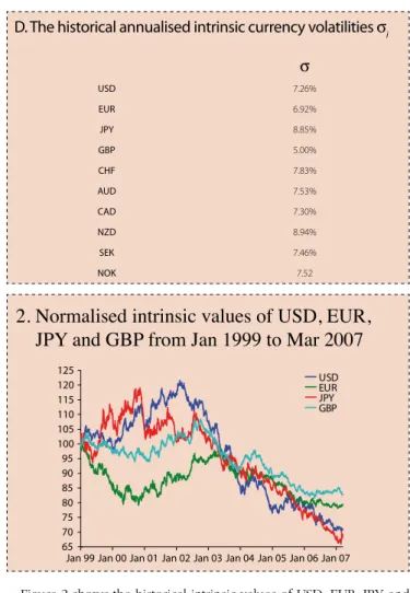
Figure 2 shows the historical intrinsic values of USD, EUR, JPY and GBP estimated using MLE. The start points are all normalised to 100 so that the movements can be seen as percentage changes. The resulting graphical representation of forex market movements is very intuitive compared with the alternative of showing the six forex rates between the currencies, which mixes the effects of each individual currency. The fact that the intrinsic values of all currencies are lower than 100 in 2007 corresponds to inflation eroding the value of all the currencies.

n The carry trade during the subprime crisis.In recent years,

an important driving force in the forex market has been the carry trade, which involves a trader borrowing money in a low interest rate currency lending in a high interest rate currency. This activity creates demand and hence strength in high interest rate currencies, with corresponding weakening in low interest rate currencies. Even though the carry trade is driven by interest rate differences that have nothing to do with the intrinsic currency calculations presented above, intrinsic currency analysis can detect activity in the carry trade because it shows the strength and weakness of individual currencies. Strengthening in high interest rate currencies with corresponding weakening in low interest rate currencies indicates trading activity going into the carry trade, while trading out of the carry trade is characterised by the opposite behaviour.

An example from summer 2007 using both the fully damped and partially damped correlation matrices is shown in figures 3 and 4.

–∆Z21 –∆Z1 –∆Z2 –∆Z21 –∆Z2 – ∆Z1 = ∆Z21 (– ____, ____)∆Z21∆Z21 2 2

In this illustrative example, we only have two currencies. They have the same variance, with ρ12 = 0 and µ = 0. The circles correspond to the contours of different probability densities. The dotted line is the constraint ∆Z2 – ∆Z1 = ∆Z21. The point on the line with the maximum likelihood is (–1/2 ∆Z21, 1/2 ∆Z21), which is the closest point to the mean

1. Maximum likelihood estimation example

Jan 99 Jan 00 Jan 01 Jan 02 Jan 03 Jan 04 Jan 05 Jan 06 Jan 07 65 70 75 80 85 90 95 100 105 110 115 120 125 _USD EUR JPY GBP

2. Normalised intrinsic values of USD, EUR,

JPY and GBP from Jan 1999 to Mar 2007

D. The historical annualised intrinsic currency volatilities

s

_i

s

USD 7.26% EUR 6.92% JPY 8.85% GBP 5.00% CHF 7.83% AUD 7.53% CAD 7.30% NZD 8.94% SEK 7.46% NOK 7.52

3 _{They are USD, EUR, JPY, GBP, CHF, AUD, CAD, NZD, SEK, NOK, CZK, SKK, PLN, HUF,}

TRY, ILS, ZAR, MXN, BRL, CLP, COP, ARS, THB, KRW, TWD, PHP, IDR, INR, SGD, CNY, HKD, RUB, XAU, XAG, HRK, KWD, PEN, PYG and ROL

During this period, the lowest interest rate currency was was JPY and the highest interest rate currency was NZD, and it is clear in both figures that the movements of JPY and NZD are mirroring each other. Together with the relatively calm performance of USD, EUR and GBP, this strongly suggests activity into the carry trade up to around July 20, 2007, and out of the carry trade thereafter. This is consistent with the commonly held belief that in late July 2007 many market participants were reducing their risk appetite. Furthermore, these results show that both the fully damped and the partially damped correlation estimation schemes produce similar results.

This example illustrates how intrinsic currency analysis can be used to answer the question ‘What currencies are ‘in play’?’. Other uses for intrinsic currency analysis include asset allocation, for example, helping investors determine the most stable currency mix, that is, the portfolios with the lowest intrinsic volatility.

n The correlations of the changes in intrinsic currency values.

Having calculated time series of intrinsic currency values, the correlations between the daily changes in the intrinsic values of the different currencies can be calculated. With the 10-currency data set, many negative correlations are found, whereas the correlations obtained from the 39-currency data set shown in table E are a reasonable match for the correlations shown in tables A and C. These

results show that using more currencies does provide more information to MLE, thus producing a more consistent correlation matrix.

n The error bars of the MLE technique. Using (19), the estimation

errors can be quantified. Table F shows the confidence intervals for using 10 and 39 currencies in the MLE. Again, the 39-currency case gives a much better estimation. Table F shows that errors accumulate as time passes. However, the same error applies to all intrinsic currency values, so the error does not affect the relative valuation of the different currencies. Also, over short time periods, the errors are relatively small and, in these cases, it is possible to quantify the percentage rises or falls in a currency’s value with reasonable accuracy.

Comparison to trade-weighted currency indexes

The idea behind trade-weighted currency indexes is to gauge the strength or weakness of a country’s currency by looking at its value relative to the currencies of its trading partners, weighted according to trade volume. Trade-related forex transactions are important because, unlike speculative transactions, they will not be subsequently unwound, and it is also trade-related transactions that act over long periods of time to drag exchange rates towards PPP exchange rates.

Formally, the trade-weighted indexes It

i for currency i at time t

are often defined (White, 1997) using:

(23)

where the trade weights wj satisfy:

and where the choice of the initial values I0

i is arbitrary. Figure 5

compares the trade-weighted index for the eurozone with the intrinsic value of EUR calculated using MLE, and it is clear that there are important differences between the two graphs.

The only consideration in constructing the It

i is to give due weight

to each of the economy’s trading partners, so that these indexes are likely to be good indicators of changes in an economy’s competitiveness that results from changes in its exchange rates with its trading partners. However, the problems with using the It

i to

gauge intrinsic currency values are that:

nThe ratios I_i/I_j have no real meaning, so taken together the I_i are

Jun 1 Jun 15 Jun 29 Jul 13 Jul 27 Aug 10 Aug 24 Sep 7 90 92 94 96 98 100 102 104 106 108 110 USD EUR JPY GBP NZD

Note: the way the graphs of JPY and NZD mirror each strongly suggests activity into and then out of the carry trade

3. Intrinsic currency values of USD, EUR, JPY, GBP

and NZD from Jun 2007 to Sep 2007 calculated

using the fully damped correlation matrix

Jun 1 Jun 15 Jun 29 Jul 13 Jul 27 Aug 10 Aug 24 Sep 7 90 92 94 96 98 100 102 104 106 108 110 USD EUR JPY GBP NZD

Note: this graph is extremely similar to figure 3, where the fully damped correlation matrix was used

4. Intrinsic currency values of USD, EUR, JPY, GBP

and NZD from Jun 2007 to Sep 2007 calculated

using the partially damped correlation matrix

E. Intrinsic currency correlations

r

_ij

, calculated from

implied forex option volatilities, averaged over the

six-month period Oct 2006–Mar 2007

USD EUR JPY GBP CHF AUD CAD NZD SEK NOK

USD 1.00 –0.02 0.27 0.16 0.01 –0.04 0.49 –0.06 –0.02 –0.02 EUR –0.02 1.00 –0.03 0.32 0.89 0.01 –0.10 0.03 0.69 0.68 JPY 0.27 –0.03 1.00 –0.05 0.07 –0.06 0.09 –0.09 –0.07 –0.02 GBP 0.16 0.32 –0.05 1.00 0.36 –0.19 –0.09 –0.12 0.20 0.20 CHF 0.01 0.89 0.07 0.36 1.00 –0.02 –0.06 0.01 0.60 0.62 AUD –0.04 0.01 –0.06 –0.19 –0.02 1.00 0.11 0.65 0.05 0.01 CAD 0.49 –0.10 0.09 –0.09 –0.06 0.11 1.00 0.04 –0.05 –0.04 NZD –0.06 0.03 –0.09 –0.12 0.01 0.65 0.04 1.00 0.03 0.01 SEK –0.02 0.69 –0.07 0.20 0.60 0.05 –0.05 0.03 1.00 0.62 NOK –0.02 0.68 –0.02 0.20 0.62 0.01 –0.04 0.01 0.62 1.00

not consistent with the forex market. This is an important flaw for market practitioners, for whom value is determined by the market. On the other hand, (2) is used as a constraint to ensure that the results of the MLE methodology are always market-consistent.

n As discussed in connection with the money quantity equation, the correlations between changes in intrinsic currency values reflect correlations between the underlying economies, as seen in tables A, C and E. However, this is not reflected in the correlations between the different I_i, which are shown in table G. The correlation between USD and CAD is a good example (–0.42 for I_i in table G and +0.49 in table E).

n Inflation erodes the value of money over time so intrinsic currency values should trend downwards in the long term. The MLE methodology incorporates this through the drifts a_i in (1), which are set to the negative of the inflation rates. However, this is not catered for in the trade-weighted index methodology (23). The effect of inflation is why the intrinsic value of EUR shown in figure 5 ends up significantly below the eurozone trade-weighted index.

For all these reasons, the MLE technique presented above is superior to using trade-weighted indexes to gauge changes in intrinsic currency values.

Conclusion

Forex market practitioners are constantly talking about the strengthening or weakening of individual currencies, and when they want to quantify such statements the usual recourse is to rely on trade-weighted currency baskets. However, the intrinsic currency methodology based on MLE presented above is much better at quantifying these statements because it is fully consistent with the

forex market, and because it reflects the intuitive correlation structure that exists between the underlying economies.

One interesting aspect of this work is the link between intrinsic currency values and the money quantity equation MV = PY in macroeconomics. It was shown that intrinsic currency values correspond to 1/P in this equation, and hence that they drift downwards over time as inflation erodes the value of money. Hyperinflation is one extreme example of this, and in this case it is clear that forex market behaviour supports this connection. A consequence of this work is a derivation for the real-world stochastic process for forex rates.

As an example, it was shown how intrinsic currency analysis was able to identify activity into and out of the carry trade from June 2007 to September 2007. Hence the method provides insight into the forex market, and consequently helps market participants trade the market better.l

Jian Chen is a quantitative analyst and Paul Doust is global head of quantitative analysis at Royal Bank of Scotland. They would like to thank Kevin Gaynor, head of economics and rates research at RBS, for valuable help in developing these ideas, as well as an anonymous referee for some valuable suggestions in connection with the economic aspects of this work, and another anonymous referee for valuable suggestions in connection with the rest. Email: [email protected], [email protected]

Jan 99 Jan 00 Jan 01 Jan 02 Jan 03 Jan 04 Jan 05 Jan 06 Jan 07 75 80 85 90 95 100 105 _{Intrinsic values} Trade-weighted index

Note: normalised to 100 at the start of January 1999

5 Intrinsic value of EUR, calculated using MLE,

compared with the corresponding trade-weighted

index

F. The confidence intervals of the MLE procedure for

different time periods

±ss (10 ccys) ±2ss (10 ccys) ±ss (39 ccys) ±2ss (39 ccys)

1D (–0.19%, 0.19%) (–0.38%, 0.38%) (–0.08%, 0.08%) (–0.15%, 0.15%)

1M (–0.90%, 0.90%) (–1.79%, 1.82%) (–0.35%, 0.35%) (–0.70%, 0.71%)

1Y (–3.05%, 3.15%) (–6.01%, 6.39%) (–1.20%, 1.22%) (–2.39%, 2.45%)

5Y (–6.69%, 7.17%) 12.93%, 14.85%) (–2.67%, 2.75%) (–5.27%, 5.57%) Note: the one- and two-standard-deviation intervals correspond to 68% and 95% confidence intervals, respectively

G. The sample correlations of the log movements of trade

weighted indexes I

_i

USD EUR JPY GBP CHF AUD CAD NZD SEK NOK

USD 1.00 –0.55 –0.42 –0.01 –0.38 –0.09 –0.42 –0.06 –0.18 –0.08 EUR –0.55 1.00 –0.31 –0.42 0.38 0.11 0.07 0.12 0.14 0.07 JPY –0.42 –0.31 1.00 –0.01 –0.05 –0.22 –0.01 –0.24 –0.07 –0.05 GBP –0.01 –0.42 –0.01 1.00 –0.09 0.01 0 0.05 –0.12 –0.07 CHF –0.38 0.38 –0.05 –0.09 1.00 –0.06 0.06 –0.03 –0.01 0.08 AUD –0.09 0.11 –0.22 0.01 –0.06 1.00 0.29 0.54 0.17 0.07 CAD –0.42 0.07 –0.01 0 0.06 0.29 1.00 0.21 0.13 0.07 NZD –0.06 0.12 –0.24 0.05 –0.03 0.54 0.21 1.00 0.08 0.08 SEK –0.18 0.14 –0.07 –0.12 –0.01 0.17 0.13 0.08 1.00 0.08 NOK –0.08 0.07 –0.05 –0.07 0.08 0.07 0.07 0.08 0.08 1.00 Blankchard O, 2005 Macroeconomics

Fourth edition, Prentice Hall

Doust P, 2007

The intrinsic currency valuation framework

Risk March, pages 76–81

Mahieu R and P Schotman, 1994 Neglected common factors in exchange rate volatility

Journal of Empirical Finance 1, pages 279–311

Mankiw N, 2006 Macroeconomics

Sixth edition, Worth Publishers

McDonald M, O Suleman, S Williams, S Howison and N Johnson, 2005

Detecting a currency’s dominance or dependence using foreign exchange network trees

Physical Review E 72, 046106

White B, 1997

The trade weighted index (TWI) measure of the effective exchange rate

Reserve Bank Bulletin 60 (2)

REFERENCES