Robust Bayesian Analysis of Loss Reserves Data Using the Generalized-t Distribution

Full text

(1)�� . QUANTITATIVE FINANCE RESEARCH CENTRE. QUANTITATIVE FINANCE RESEARCH CENTRE Research Paper 196. May 2007. Robust Bayesian analysis of loss reserves data using the generalized-t distribution Jennifer Chan, Boris Choy and Udi Makov. ISSN 1441-8010. www.qfrc.uts.edu.au.

(2) Robust Bayesian analysis of loss reserves data using the generalized-t distribution. By Jennifer S.K. Chan School of Mathematics and Statistics The University of Sydney, Australia Email: [email protected] S.T. Boris Choy Department of Mathematical Sciences University of Technology Sydney, Australia Email: [email protected] and Udi E. Makov Department of Statistics, University of Haifa, Israel Email: [email protected]. Abstract: This paper presents a Bayesian approach using Markov chain Monte Carlo methods and the generalized-t (GT) distribution to predict loss reserves for the insurance companies. Existing models and methods cannot cope with irregular and extreme claims and hence do not offer an accurate prediction of loss reserves. To develop a more robust model for irregular claims, this paper extends the conventional normal error distribution to the GT distribution which nests several heavytailed distributions including the Student-t and exponential power distributions. It is shown that the GT distribution can be expressed as a scale mixture of uniforms (SMU) distribution which facilitates model implementation and detection of outliers by using mixing parameters. Different models for the mean function, including the log-ANOVA, log-ANCOVA, state space and threshold models, are adopted to analyze real loss reserves data. Finally, the best model is selected according to the deviance information criterion (DIC). Keywords: Bayesian approach, state space model, threshold model, scale mixtures of uniform distribution, deviance information criterion.. - 1-.

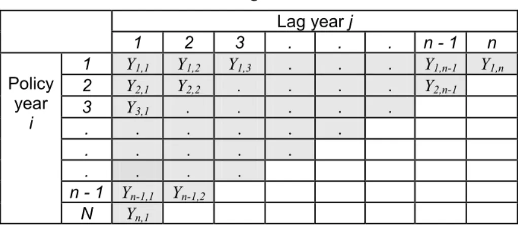
(3) 1. Introduction An insurance policy is a promise of an insurance company to pay claims to the insureds if some defined events (death, accident, injury, etc.) occur. However in many cases, claims originating in a particular year are often not settled in that year, but with a time delay of years or perhaps decades. Therefore, the insurance company must have the necessary loss reserves to pay these outstanding claims and settlement costs incurred. With many uncertainties in the time lags inherently involved in the claims settlement process, the estimation procedure of the required loss reserves is extremely complicated. Since loss reserves generally represent by far the largest liability and the greatest source of financial uncertainty in an insurance company, accurate prediction of the loss reserves is of great importance. Failure to estimate the loss reserves accurately may result in large profit losses and hence weaken the financial stability of the company which may ultimately drive it into insolvency.. Denote Yi,j, i, j = 1, K , n, the value of claims paid by an insurance company for accidents that. occurred in policy year i and were settled after j -1 years (lag year j ). The observed claim amounts Yi,j, i = 1, K , n, j ≤ n − i + 1 over a period of n policy years can be presented by a run-off triangle; see Table 1. The total number of observed claims in the upper triangle is SU =. n(n + 1) and the number of unobserved claims to be predicted in the lower triangle is 2. n(n − 1) . The aim is to predict the unobserved values in the lower triangle using an 2 appropriate statistical model. SL =. Table 1. Run-off triangle for claim data. 1 Y1,1 1 Policy Y2,1 2 year Y3,1 3 i . . . . . . n - 1 Yn-1,1 Yn,1 N. 2 Y1,2 Y2,2 . . . . Yn-1,2. 3 Y1,3 . . . . .. - 2-. Lag year j . . . . . . . . . . .. . . . .. n-1 Y1,n-1 Y2,n-1. n Y1,n.

(4) The most popular method for prediction is the chain-ladder method (Renshaw, 1989) which uses loss ratio estimate and loss development factors. However it is increasingly apparent that this method lacks some measures of variability. Over the years, stochastic models with hierarchical structure have been developed to overcome such shortcomings. For example, Verrall (1991, 1996) and Renshaw and Verrall (1998) adopt the ANOVA-type and ANCOVA-type models. The interaction between the policy year and lag year prompted the development of the state space models which allow dynamic evolution of parameters in a time-recursive way. See Verrall (1989, 1994). In addition, Hazan and Makov (2001) propose the threshold models to allow for structural changes in the trend of outstanding claims over time. Analyses of real data suggest that the dynamic nature of the state space model and threshold model improves the prediction. It is well known that the normal error distribution falls short of allowing for irregular and extreme claims and hence contaminates the estimation procedure and leads to poor prediction. To allow for irregular claims, error distributions that possess flexible tails are recommended. The Student-t distribution has been widely used by many researchers for this purpose while Choy and Chan (2003) use the exponential power (EP) family of distributions. In this paper, we shall adopt the generalized-t (GT) distribution (McDonald and Newey, 1988) for the errors. The GT distribution is symmetric and is governed by two shape parameters. By suitably choosing these shape parameter values, one can easily show that the normal, Cauchy, Student-t, EP and Laplace distributions are members of the GT family. For a long time the Bayesian approach had very limited applications in statistical inference because the posterior functionals that involve high-dimensional integration cannot be obtained analytically. Gelfand and Smith (1990) develop the simulated-based Markov chain Monte Carlo (MCMC) techniques that transform the integration problem into a sampling problem. The idea is to construct a Markov chain whose limiting distribution is the intractable joint posterior distribution. The simulated realizations from the Markov chain mimic a random sample from the joint posterior distribution and the posterior functionals can be estimated from these realizations. Amongst the MCMC algorithms, Gibbs sampling (Geman and Geman, 1984), Metropolis-Hastings (Metropolis et al., 1953 and Hastings, 1970) and Reversible Jump MCMC (Green, 1995) are very common. Bayesian statistical inferences can be easily done using WinBUGS (Spiegelhalter et al., 2004), an easy-to-use software for MCMC algorithms. Readers who are interested in or unfamiliar to WinBUGS may find the educational materials on the official WinBUGS website very useful. See www.mrcbsu.cam.ac.uk/bugs/welcome.shtml. They are referred to Gilks et al. (1998) and Gelman et al. (2004) for MCMC applications in many statistical problems. For actuarial and insurance applications, see, for example, Makov (2001), De Alba (2002), Ntzoufras and Dellaportas (2002), Ntzoufras et al. (2005), Scollnik (1998, 2001, 2002) and Verrall (2004). - 3-.

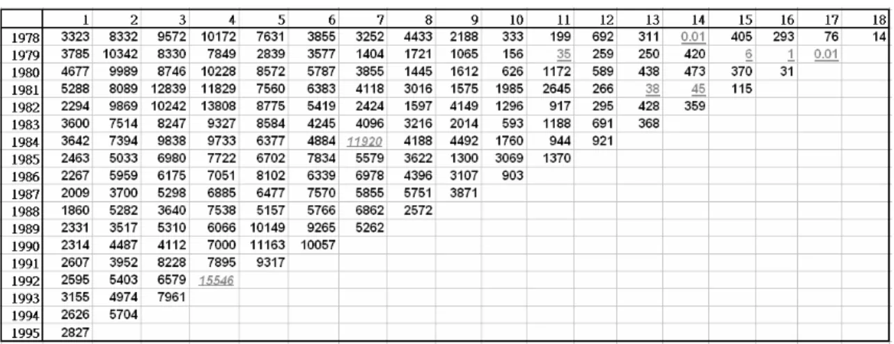
(5) To simplify the computational procedure for the Bayesian calculation and to speed up the Gibbs sampling algorithm, the GT error distribution is expressed into a scale mixtures representation. The GT distribution can be expressed as a scale mixture of uniforms (SMU) distribution as all of its constituting families of distributions, the EP and Student-t distributions, can be expressed as SMU distributions. This paper makes the first attempt to adopt the GT error distribution via the SMU form for model implementation and to protect inferences from possible outliers that can be detected using the mixing parameters of the SMU representation. The rest of this paper is structured as follows. Section 2 introduces the data that demonstrate the proposed loss reserve models. Section 3 reviews the models with normal error distribution. Section 4 outlines the GT distribution and its scale mixtures representations. Section 5 implements the models using the Bayesian approach and proposes the DIC for choosing the best model. Section 6 reports and compares the results. Finally, discussion of results and further research direction is outlined in Section 7. 2. The data. To demonstrate the models proposed in Sections 2 and 3, a loss reserve data set as shown in Table 2 is analyzed. The data are the amount of claims paid to the insureds of an insurance company during the period of 1978 to 1995 over n = 18 years. The upper triangle has N = 171 observations and the 153 observations in lower triangle are not yet observed. For mathematical convenience, two zero claim amounts are replaced by 0.01. Some general trends are obvious. Figure 1(a) shows that given a policy year, the amount of claims paid follows an increasing trend in the first 4 to 6 lag years and then a decreasing trend thereafter. On the other hand, Figure 1(b) shows no obvious trends for each lag year. This data set contains some extreme outliers which are underlined in Table 2. For example, extremely large claims (in italic), amount to 11920 and 15546 dollars, were made in the 7-th lag year of policy year 1984 and in the 4-th lag year of policy year 1992 respectively. These outliers distort the general trends in the data and inflate the standard errors of the model parameters. Other outliers have much smaller amount of claims than their neighboring claims. These claims may lead to underestimates of loss reserves and hence lower the solvency and increase the risk of bankruptcy for an insurance company. Hence for robustness consideration, heavy-tailed error distributions are adopted to accommodate these irregular claims.. - 4-.

(6) Table 2. The amount of claims paid to the insureds of an insurance during 1978 to 1995.. Figure 1 (a) Claim amounts across policy years. (b) Claim amounts across lag years. Amount of loss across policy year. Amount of loss across lag year. 16000 14000 10000. Amount. Amount. 12000 8000 6000 4000 2000 0 1. 2. 3. 4. 5. 6. 7. 8. 18000 16000 14000 12000 10000 8000 6000 4000 2000 0 1. 9 10 11 12 13 14 15 16 17 18. 2. 3 4. 5. 6 7. 1979 1983 1987. 1980 1984 1988. 9 10 11 12 13 14 15 16 17 18. Policy ye ar. Lag ye ar. 1978 1982 1986. 8. 1981 1985. lag1. lag2. lag3. lag7. lag8. lag9. lag4. lag5. lag6. 3. Modeling the mean function. The popular log-linear model was investigated by Renshaw (1989), Verrall (1991, 1996) and Renshaw and Verrall (1998) in actuarial context. Depending on the formulation of policy year and lag year effects, we consider the log-ANOVA, log-ANCOVA and state space models for the mean function. For the state space model, the interaction effects between the policy-year and the lag-year are assumed. Each of these models is then allowed to switch to the model with a new set of parameters after certain thresholds. All models are implemented using WinBUGS with vague and non-informative prior distributions assigned to the model parameters. 3.1 ANOVA models. Within the Bayesian hierarchical modeling framework, the log-adjusted claim amount μ ij , written in year i and paid with a delay j-1 years, adopts a two-way ANOVA model with normal error distribution where μ ij is the mean function, α i is the policy year effects and β i is the lag year effects as below:. log(Yij ) = μ ij + ε ij. (1). μij = μ + α i + β j. (2). - 5-.

(7) ε ij ~ N (0, σ 2 ). (3). for i = 1, K , n, j ≤ n − i + 1 subject to the constraints. ∑. n i =1. α i = ∑ j =1 β j = 0. To complete the n. Bayesian framework, we adopt the following priors for the model parameters:. μ ~ N (0, σ μ2 ) , α i ~ N (0, σ α2 ) , β j ~ N (0, σ β2 ) , σ 2 ~ IG (a, b) where IG (a, b) is the inverse gamma distribution with density a +1. ba ⎛ 1 ⎞ ⎛ b ⎞ ⎜ 2 ⎟ exp⎜ − 2 ⎟ . Γ(a ) ⎝ σ ⎠ ⎝ σ ⎠ Diffuse priors can be obtained by setting the hyperparameters σ μ2 = σ α2 = σ β2 = ∞ and a = b = 0 , f (σ 2 ) =. i.e. inflating the variances of the prior distributions to reflect the lack of prior information (Ntzoufras and Dellaportas, 2002). In this case, the joint prior density is p ( μ , α , β, σ 2 ) ∝. 1. σ2. where α = (α1 ,K.α n ) and β = ( β1 ,K, β n ). 3.2 ANCOVA model. In the ANCOVA model, the effects of policy year i and lag year j are linear. The three different combinations of effects are given below. 1. Linear effect of policy year and categorical effect of lag year, 2. Categorical effect of policy year and linear effect of lag year and 3. Linear effect of both policy year and lag year. Preliminary result of the analysis reveals that the first combination provides the best fit to the data and hence is chosen for all subsequent analyses of the ANCOVA model. Analysis of the model follows from the log-ANOVA model from (1) to (3) except that the mean function becomes. μ ij = μ + α ⋅ i + β j for i = 1, K , n, j ≤ n − i + 1 subject to the constraints. (4). ∑. n j =1. β j = 0. The diffuse priors are. chosen to be p ( μ , α , β, σ 2 ) ∝ where β = ( β1 ,K, β n ).. 1. σ2. 3.3 State space model. To account for the interaction between the policy year and lag year in the mean function, the state space model (Ntzoufras and Dellaportas, 2002, De Jong and Zehnwirth, 1983 and Verrall, 1991, 1994) is considered. In the model, parameters are allowed to evolve in a timerecursive pattern: α i depends on α i −1 and an error term hi while β ij depends on β i −1, j and an error term vi . The model again follows from log-ANOVA model from (1) to (3) except that the mean function becomes - 6-.

(8) μ ij = μ + α i + β ij. (5). for i = 1, K , n, j ≤ n − i + 1 where the recursive associations are. α i = α i −1 + hi ,. hi ~ N (0, σ h2 ),. i = 2,3, ..., n. (6). β ij = β i −1, j + vi ,. vi ~ N (0, σ v2 ),. i, j = 2,3, ..., n. (7). subject to the constraints α1 = 0 and β i1 = 0 for i = 1, K , n . The priors for σ h2 and σ v2 follow. σ h2 ~ IG (ah , bh ) and σ v2 ~ IG (av , bv ) respectively. Diffuse prior distributions for the parameters are chosen to be. p( μ , β1 , σ 2 , σ h2 , σ v2 ) ∝. 1. σ σ h2σ v2 2. where β1 = ( β12 ,K, β1n ). 3.4 Threshold model. Hazan and Makov (2001) suggested a switching regression model in which the mean functions before and after a threshold T along the axis of policy year are assigned the same model but with a different set of parameters. The reasoning behind is that some events such as a financial crisis or a change in the insurance regulation may take place on or before certain threshold year T. These events may change the effects of some factors on the claim amounts and hence a new set of parameters is adopted to reveal such changes. The threshold models based on different mean function structures are given below: Threshold log-ANOVA model:. Threshold log-ANCOVA model:. Threshold state space model:. μ ij = μ1 + α 1i + β1 j μ ij = μ 2 + α 2i + β 2 j μij = μ1 + α1 × i + β1 j μij = μ2 + α 2 × i + β 2 j μ ij = μ1 + α1i + β1ij μ ij = μ 2 + α 2i + β 2ij. for i < T for i ≥ T , j ≤ n – T+1 for i < T for i ≥ T , j ≤ n – T+1 for i < T. (8). for i ≥ T , j ≤ n – T+1 (9). The main difference in these threshold models is related to the set of β parameters which change after the threshold policy year T. On the contrary, the criterion that the α parameters are different before and after the threshold also holds for the simple models. Prior distributions for the parameters in the three models remain the same as those in Sections 3.1 to 3.3. The threshold T can be selected based on some model selection measures such as the Akaike information criterion (AIC) (Akaike, 1974), the Bayesian information criterion (BIC) (Schwarz, 1978), the Deviance information criterion (DIC) (Gelman et al., 2004) and the posterior expected utility U (Walker and Gutiérrez-Peña, 1999). We will use the DIC in this paper because it is particularly useful in Bayesian model selection problems where the posterior distributions of the model parameters have been obtained by MCMC simulation. Threshold models with threshold lag-years, for example, Threshold log-ANOVA model:. μ ij = μ1 + α 1i + β1 j μ ij = μ 2 + α 2i + β 2 j - 7-. for j < T , for j ≥ T , i ≤ n – T+1,.

(9) are also possible. However they are not considered further in this paper as the loss reserves data in the numerical illustration show no clear trends of claim amounts across policy years for each given lagyear (see Figure 1b). 4. Error distributions. Past experience has shown that irregular claims which often present in loss reserve data may seriously distort the parameter estimates and hence affect the accuracy of the prediction. The traditional log-linear models with normal errors fall short of allowing for the irregularities in the claim amounts. Heavy-tailed distributions such as the Cauchy, Student-t, Laplace and EP distributions are adopted for the errors in order to robustify the statistical inferences. However searching across these error distributions for the most suitable distribution, though workable, is timeconsuming. The GT distribution, nesting all these competing heavy-tailed distributions as well as lighter-tailed alternatives including the popular normal and uniform distributions, provides a favorable choice for the error distribution (Butler et al., 1990). 4.1 Generalized-t distributions. Proposed by McDonald and Newey (1988), the GT distribution is symmetric and unimodal and has a probability density function (PDF). p. GT ( x | μ , σ , p, q ) =. 1 ⎛1 ⎞⎛ 1 x−μ 2 q p σ Β⎜⎜ , q ⎟⎟ ⎜1 + ⎝ p ⎠ ⎜⎝ q σ. p. ⎞ ⎟ ⎟ ⎠. q+. 1 p. (10). where μ ∈ ℜ is a location parameter, σ > 0 is a scale parameter, p > 0 and q > 0 are two shape parameters and B(⋅) is the beta function. When μ = 0 and σ = 1, the rth moment of the GT distribution is given by r p. ⎛ r + 1⎞ ⎛ r⎞ ⎟⎟ Γ⎜⎜ q − ⎟⎟ q Γ⎜⎜ p⎠ ⎝ p ⎠ ⎝ E[ X r ] = ⎛1⎞ Γ⎜⎜ ⎟⎟ Γ(q ) ⎝ p⎠. provided that r < pq.. In particular, the variance is given by 2 p. ⎛3⎞ ⎛ 2⎞ q Γ⎜⎜ ⎟⎟ Γ⎜⎜ q − ⎟⎟ p⎠ ⎝ p⎠ ⎝ V[X ] = ⎛1⎞ Γ⎜⎜ ⎟⎟ Γ(q ) ⎝ p⎠. provided that pq > 2.. The tail behavior and other characteristics are controlled by p and q. Large values of p and q signify distributions with thinner tails than the normal distribution whereas small values of p and q signify distributions with thicker tails. Hence the GT distribution can accommodate both leptokurtic and platykurtic distributions. The GT family includes several important distributions: the normal ( p = 2, q → ∞) , the Cauchy ( p = 2, q = 1 / 2) , the Student-t with 2q degrees of freedom ( p = 2) , the Laplace ( p = 1, q → ∞) , the EP with shape parameter p (q → ∞) , and the uniform ( p → ∞) distributions. When p = 2 , the PDF in (10) reduces to. - 8-.

(10) ⎛ν + 1 ⎞ Γ⎜ ⎟ ⎝ 2 ⎠. t ( x | μ ,τ ,ν ) =. 2 ⎛ν ⎞ ⎛ ( x − μ ) τ νπ Γ⎜ ⎟ ⎜⎜1 + τ 2ν ⎝2⎠ ⎝. ⎞ ⎟⎟ ⎠. ν +1 2. which is the PDF of the Student-t distribution with degrees of freedom ν = 2q and scale parameter τ = σ parameter p. 2 . Moreover, (10) converges to the PDF of the EP distribution with shape. ⎛ x−μ p⎞ ⎟ exp⎜ − ⎟ ⎜ σ ⎠ ⎝ EP ( x | μ , σ , p ) = ⎛ 1⎞ 2 σ Γ⎜⎜1 + ⎟⎟ p⎠ ⎝. when q → ∞ . Lastly, (10) also converges to the PDF of the uniform distribution. U ( x | μ,σ ) =. 1 I ( x ∈ ( μ − σ , μ + σ )) 2σ. when p → ∞ . In addition, when p ≤ 1, the GT distribution is cuspidate. Figure 2 summarizes the relationship amongst the well-known distributions within the GT family. Figure 9 (a)-(e) in Appendix B gives the PDFs for different values of p and q when μ = 0 and σ = 1 . Figure 2: The GT distribution family tree.. 3.2 Scale mixtures of uniform distributions. 4.2 The generalized gamma distribution. 4.2 The Generalized gamma distributions. The generalized gamma (GG) distribution with parameters α , β , γ > 0 , denoted by. GG(α , β , γ ), has a PDF given by GG ( x | α , β , γ ) =. γβ αγ αγ −1 x exp(− β γ x γ ) Γ(α ). - 9-.

(11) where β is a scale parameter and α and γ are shape parameters. The sth moment of the distribution is. E[ X s ] =. (. ). Γ α + s γ −1 . β s Γ(α ). The GG distribution includes the Weibull ( α = 1 ), gamma ( γ = 1 ), exponential ( α = γ = 1 ) and lognormal ( α = 0 ) distributions as special cases. In particular, when γ = 1 , the GG distribution reduces to the gamma Ga(α , β ) distribution having the PDF. Ga ( x | α , β ) = the mean E[ X ] =. β α α −1 x exp(− β x ) , Γ (α ). α α and the variance V [ X ] = 2 . For inferential procedures for the GG β β. distribution, see Hager and Bain (1970). See also McDonald and Butler (1987) for the applications in finance. 4.3 The scale mixtures representation of the GT distribution. Recently, Arslan and Genc (2003) showed that the GT distribution can be expressed into a scale mixtures of Box and Tiao distribution (Box and Tiao, 1962), or the scale mixtures of exponential power (SMEP) distribution because the Box and Tiao distribution is another name for the EP distribution. Using the SMEP density representation, the PDF in (10) can be rewritten as. (. ). ∞ ⎛ p⎞ GT ( x | μ , σ , p, q) = ∫ EP x μ , q1 / p s −1 / 2σ , p GG⎜⎜ s q,1, ⎟⎟ ds . 0 2⎠ ⎝. (11). The latent variable, s, arises in the above expression is called the mixing variable of the SMEP density representation and has a GG (q,1, p / 2) distribution. Similar to the mixing variables of the scale mixtures of normal (SMN) distributions (Choy and Smith, 1997) and the scale mixtures of uniform (SMU) distributions (Choy and Chan, 2003), the mixing variable s in (11) can be used as a global diagnostic of possible outliers. Small mean value of s associates with possible outlier because the corresponding EP distribution in (11) must inflate its variance to accommodate the outlier. See Choy and Smith (1997) and Choy and Chan (2003) for outlier diagnostics using the mixing variable of the SMN and SMU distributions, respectively. Many symmetric and non-normal distributions are extremely difficult to handle in statistical inference because of the non-conjugate structure of the models. In Bayesian computation, expressing the PDF of a distribution into a certain kind of scale mixtures form enables efficient simulation-based algorithms. Without using a scale mixtures representation, sampling non-standard full conditionals in Bayesian Gibbs sampling procedure relies on the Metropolis-Hastings algorithm, the slice sampler (Damien et al., 1999) or other simulation algorithms. However, the Metropolis-Hastings algorithm and some other simulation algorithms require expertise in simulation techniques to provide reliable and efficient algorithms. The slice sampler is an easy-to-use algorithm that introduces an auxiliary variable to reduce a non-standard full conditional in a Gibbs sampler to standard full conditionals. However, there is no physical meaning for the auxiliary variable. On the contrary, the use of a scale mixtures density representation for a non-normal distribution - 10 -.

(12) results in adding extra latent variables in the model and hopefully produces a set of standard full conditionals for the Gibbs sampler. In addition, these latent variables are used to identify possible outliers. Therefore, the slice sampler and the use of scale mixtures density representation play different roles in Gibbs sampling even though they both use latent variables. Although the GT distribution can be expressed as a SMEP distribution, the EP distribution is difficult to handle analytically in statistical inference because its density function involves an absolute term. Walker and Gutiérrez-Peña (1999) showed that the EP distribution can be expressed as a SMU distribution and Choy and Chan (2003) successfully adopt this SMU representation of the EP distribution in an insurance application. In this paper, we combine the SMEP for the GT distribution and the SMU for the EP distribution to obtain a SMU representation for the GT distribution. The resulting Gibbs sampler can be shown to have a set of easily sampled standard full conditional distributions. be a gamma Ga (1 + 1 / p , 1) random variable where the PDF of the. Let U. Ga (a, b) distribution is b a a −1 −bu Ga (u | a, b) = u e Γ(a ) and the mean and variance are E[U ] =. u , a, b > 0. a a and V [U ] = 2 , respectively, and S be a b b. ⎛p ⎞ ,1, q ⎟ random variable. Then, if X is a GT random variable ⎝2 ⎠. generalized gamma GG ⎜. with parameters μ , σ , p and q, we have. −1 −1 X | U = u , S = s ~ Unif ⎛⎜ μ − q p s 2 u p σ , μ + q p s 2 u p σ ⎞⎟ ⎠ ⎝ 1. 1. 1. 1. ⎛ 1 ⎞ U ~ Ga⎜⎜1 + , 1⎟⎟ p ⎠ ⎝ p⎞ ⎛ S ~ GG ⎜ q,1, ⎟ . 2⎠ ⎝. and. In other words, the PDF in (10) can be rewritten as ∞. ∞. ∫ ∫φ 0. 1 1 1 1 ⎛ 1 ⎞ −1 −1 ⎛ p ⎞ Unif ( x | μ − q p s 2 u p σ , μ + q p s 2 u p σ )Ga ⎜⎜ u | 1 + , 1⎟⎟ GG ⎜ s | ,1, q ⎟ du ds p ⎠ ⎝ 2 ⎠ ⎝. where. 1 x−μ φ = q σ. p. p 2. s .. 2/ p 2 The conditional variance of the above uniform distribution is (qu ) σ /(3s ) which inflates with a large u and a small s . To identify potential outliers, we propose to use the ratio. - 11 -.

(13) ψ = u 1 / p s −1 / 2 because it controls the support and hence the variance of the uniform distribution. Hence the sampling is performed with the observed data x and the mixing parameters u and s which are used for identification of outliers. Although the number of parameters to be sampled becomes larger with the inclusion of mixing parameters, sampling can be conducted more efficiently from standard full conditional distributions. Hence the SMU representation simplifies the computational procedures for Bayesian calculation and speeds up the Gibbs sampling algorithm in WinBUGS as designated. 5. Bayesian analysis 5.1 Model implementation. Bayesian approach is adopted for parameter estimation and is performed using WinBUGS. Command codes for the implementations are given in the Appendix A. Parameters are estimated from samples drawn from the posterior conditional distributions. Due to the complexity of the models, high posterior correlations exist between some parameters. These dependences may slow down the convergence rate in the Gibbs samplers for some parameters. As a result, the number of iterations M should be large enough to ensure that the sample is uncorrelated, large and stationary. We set M = 105,000 and the burn-in period is at least 5,000 iterations. After the burn-in period, parameters are taken from every 50th iteration to mimic a random sample of size at least K = 1,000 from the intractable joint posterior distribution. Trajectory plots and autocorrelation plots of the simulated values are used to check for the independence and convergence of the sample. The posterior sample means, or medians where appropriate, are reported as parameter estimates. 5.2 Model Selection. To choose the most appropriate Bayesian model for the loss reserves data, the Deviance information criterion (DIC) is used. The DIC is proposed by Spiegelhalter, et al. (2002) as a model selection method for complex hierarchical models in which the number of parameters is not clearly defined. The DIC is defined as. DIC = E[ D(θ )] + ΔD(θˆ) where E[ D(θ )] is a measure of the adequacy of model fitting and ΔD(θˆ) = E[ D(θ )] − D(θˆ) estimates the effective number of parameters in the model. Based on the posterior sample, we calculate the DIC as. ⎛ 2 1000 n n−i +1 ⎞ 1 n n−i +1 DIC = −2⎜⎜ ∑∑ ∑ ln f ij ( zij | θ k ) − ∑ ∑ ln f ij ( zij | θˆ ) ⎟⎟ N i =1 j =1 ⎝ N k =1 i =1 j =1 ⎠ where zij = ln yij is the log claim size, f ij (⋅) is the GT density function given by (10) when the mean μ is replaced by μ ij in (2), (4) and (5) for the log-ANOVA, log-ANCOVA and state space models respectively, θ k is a vector of all parameters in the kth posterior sample and θ̂ is a vector of posterior means or medians of all parameters. Obviously a model with the smallest DIC is the best model. - 12 -.

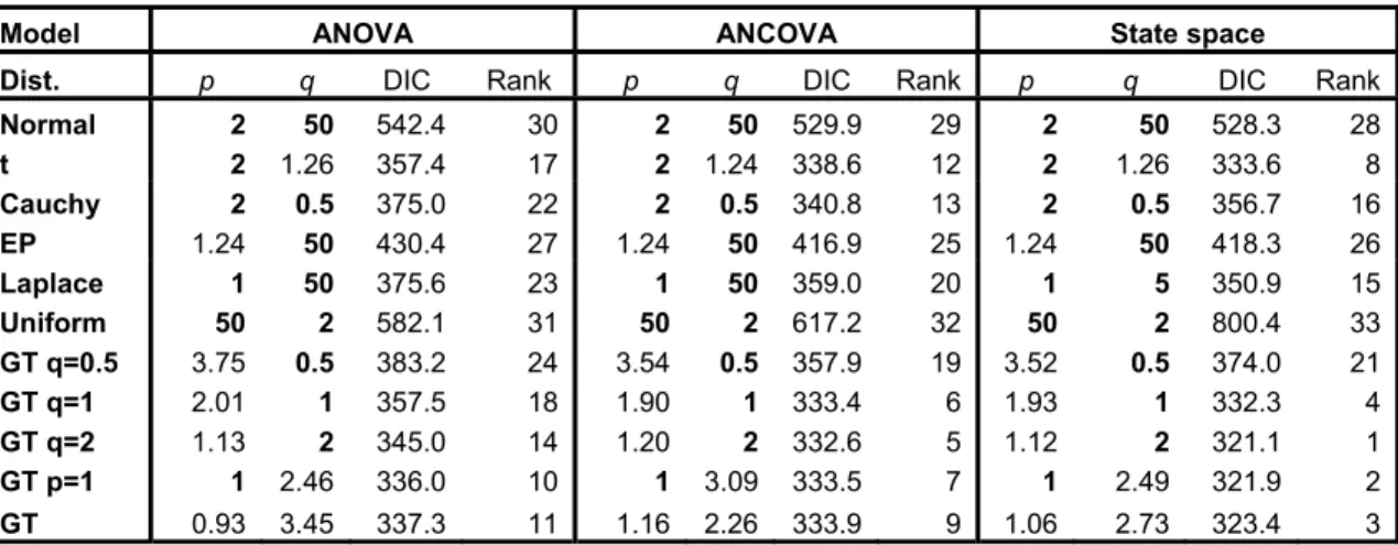
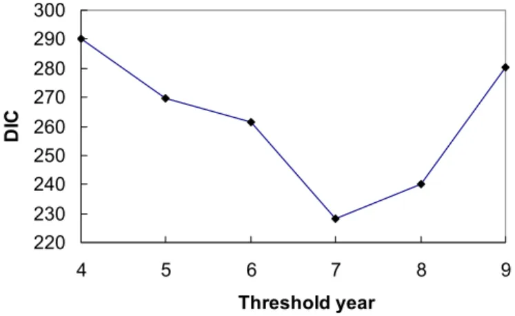
(14) 6. Results 6.1 Comparison between mean functions and error distributions. Various models with different mean functions and error distributions are fitted to the claim data. For each type of mean function, we set the two shape parameters, p and q, of the GT distribution to take different values, which signify different distributions that are nested within the GT family. In the simulation study, we set p = 50 to approximate the uniform distribution and q = 50 to approximate the EP distribution which includes the normal and Laplace distributions. From (10), these values for p and q approximate the limiting cases of p → ∞ and q → ∞ well. Moreover, more general families of distributions can be obtained by setting either p or q or both to be random. For example, p = 1 and q is random, and p is random and q = 0.5, 1 and 2, respectively, are used in the simulation study. Models are ranked according to DIC. Table 3 exhibits the DIC values for a wide choice of error distributions for the log-ANOVA, logANCOVA and state space models. For the log-ANOVA model, the most appropriate error distribution is the GT distribution with p = 1 and q being random. The posterior mean of q is 2.46. For the log-ANCOVA and state space models, the GT error distribution with a random p and q = 2 is chosen and the posterior medians of p are 1.20 and 1.12, respectively. These p and q values correspond to the GT distributions that are heavier-tailed than the normal distribution. The DIC values for these three models are 336.0, 332.6 and 321.1, respectively and the state space model with a random p and q = 2 is preferred amongst the models studied. Table 3. Goodness-of-fit measures for models with different mean functions and error distributions. Bold types values correspond to fixed parameter values. Model. ANOVA. ANCOVA Rank. State space. Dist.. p. q. DIC. q. DIC. q. DIC. Normal t Cauchy EP Laplace Uniform GT q=0.5 GT q=1 GT q=2 GT p=1. 2 2 2 1.24 1 50 3.75 2.01 1.13 1. 50 1.26 0.5 50 50 2 0.5 1 2 2.46. 542.4 357.4 375.0 430.4 375.6 582.1 383.2 357.5 345.0 336.0. 30 17 22 27 23 31 24 18 14 10. 2 2 2 1.24 1 50 3.54 1.90 1.20 1. 50 1.24 0.5 50 50 2 0.5 1 2 3.09. 529.9 338.6 340.8 416.9 359.0 617.2 357.9 333.4 332.6 333.5. 29 12 13 25 20 32 19 6 5 7. 2 2 2 1.24 1 50 3.52 1.93 1.12 1. 50 1.26 0.5 50 5 2 0.5 1 2 2.49. 528.3 333.6 356.7 418.3 350.9 800.4 374.0 332.3 321.1 321.9. 28 8 16 26 15 33 21 4 1 2. GT. 0.93. 3.45. 337.3. 11. 1.16. 2.26. 333.9. 9. 1.06. 2.73. 323.4. 3. p. Rank. p. Rank. 6.2 Comparison between simple and threshold models. To allow for structural changes in the trend of claim amount over time, threshold model that assumes a structural change at policy year T is suggested. For the loss reserve data used throughout this paper, state space model is shown to perform better than the log-ANOVA and log-ANCOVA models across a wide choice of error distributions in general. Therefore, the state space threshold model is used to re-analyze the claim data in this section. The threshold T is fixed within the range (1, n) for the policy year, not too close to either sides of the range. The mean function takes two different sets of parameters – one set before T and the other set on and after T. Table 4 exhibits the posterior medians and posterior standard deviations of p, q and DIC of various state space threshold models. Figure 3 displays the change of DIC versus - 13 -.

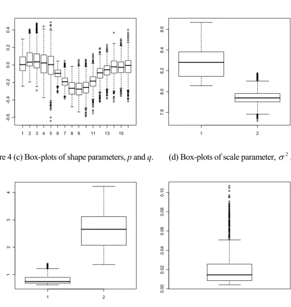
(15) T. The state space model with threshold year T = 7 (year 1984) is shown to be the most appropriate model (DIC = 228.3). The posterior medians of p and q of the GT distribution are p̂ = 0.81 and q̂ = 2.63, respectively. This threshold model is chosen for the loss reserve prediction.. Table 4. Posterior medians of p and q (standard deviations in parentheses) and DIC for different state space threshold models. Threshold p q DIC. T =4. T =5. T =6. T =7. T =8. T =9. 1.19 (0.16) 2.12 (0.45) 290.3. 0.84 (0.10) 2.77 (0.48) 269.8. 0.79 (0.07) 3.12 (0.64) 261.6. 0.81 (0.16) 2.63 (0.61) 228.3. 0.84 (0.08) 2.56 (0.47) 240.3. 0.79 (0.10) 2.93 (0.58) 280.2. Figure 3. DIC versus threshold year, T for different state space threshold models. 300 290 280 DIC. 270 260 250 240 230 220 4. 5. 6. 7. 8. 9. Threshold year. Figure 4 gives the box-plots of all model parameters in the posterior samples for the chosen model except the beta parameters, β ij , which have too many parameters. The alpha and beta parameters in (8) and (9) are given by (6) and (7) respectively before and after the threshold year of 1984. The beta parameters for each policy year form a periodic trend across lag years: they increase up to lag years 4 to 6 and then decrease. Moreover the beta parameters at higher lag years have larger variability due to the insufficiency of observations to estimate the parameters accurately. Box-plots of alpha parameters also show trends of increasing variances across policy years before and after 1984 (the first five box-plots and the remaining box-plots respectively).. - 14 -.

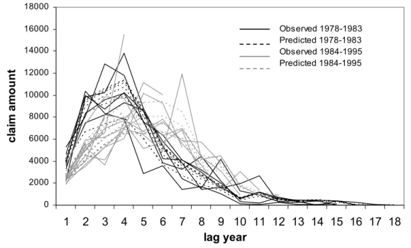
(16) (b) Box-plots of mu parameters, μ ki .. -0.6. 7.8. -0.4. 8.0. -0.2. 8.2. 0.0. 8.4. 0.2. 0.4. 8.6. Figure 4 (a) Box-plots of alpha parameters, α i .. 1. 2. 3. 4. 5. 6. 7. 8. 9. 11. 13. 15. 1. 2. (d) Box-plots of scale parameter, σ 2 .. 0.00. 1. 0.02. 0.04. 2. 0.06. 3. 0.08. 4. 0.10. Figure 4 (c) Box-plots of shape parameters, p and q.. 1. 2. Table 6 reports the predicted claims in the upper triangle. Claims in italic refer to the predicted claims from policies written on and after 1984. Claims underlined are predicted from claims which are extremely low or high (in italic) in values as compared with neighboring claims. The observed claims (Table 2) in solid line and the predicted claims in dotted line are plotted in Figure 5. The figure shows clearly two different trends of claims before and after 1984 as indicated by the black and grey lines respectively. For claims from policies written before 1984, the predicted claims increase with the lag year till the 4th lag year and drop slowly thereafter. For policies written on and after 1984, the predicted claims start from lower levels, rise to the lower maximums at the 6th lag year and drop more rapidly thereafter. In general, the predicted claims (dotted lines) lie close to the observed claims showing that the chosen model fits the data well.. - 15 -.

(17) Table 6. Run-off triangle of predicted and projected levels of claims using the chosen model.. Values in italic are estimated or predicted claims from policies written after 1984. Values in black and underlined are predicted claims for outliers (predicted claims from large outliers are in italic). Values in grey and purple in the lower triangle are projected claims. Values in underlined in the lower triangle are projected claims with standard errors higher than half of the values. Values in purple are projected claims estimated using (12).. Table 7. Total projected outstanding claims for each policy year and their standard errors.. Figure 5. Observed and predicted claim amounts using the chosen model, the state space threshold model with a GT error distribution (T = 7 and p and q are random). 18000 Observed 1978-1983 Predicted 1978-1983 Observed 1984-1995 Predicted 1984-1995. 16000. claim amount. 14000 12000 10000 8000 6000 4000 2000 0. 1. 2. 3. 4. 5. 6. 7. 8 9 10 11 12 13 14 15 16 17 18 lag year. Projection for the outstanding claims in the lower triangle of Table 2 using the chosen model is reported in Table 6. The values are the posterior medians of the projected claims using the - 16 -.

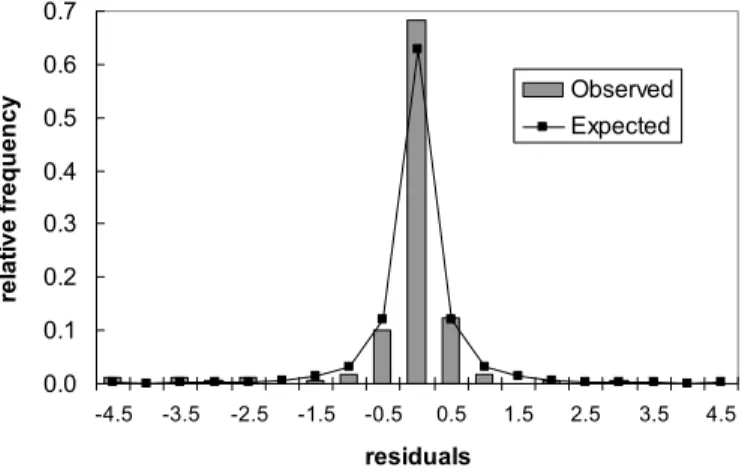
(18) K = 1,000 sets of parameter estimates. The projected total outstanding claims, as the posterior median of the 1000 sums of projected claims, is 296,159 dollars with an estimated standard error of 123,867 dollars. The projected total outstanding claims for each policy year and their standard errors are reported in Table 7. Note that the projected claims Yîj , i ≥ 7, j ≥ 13 ,. written in purple in Table 6, are estimated using. β 2,ij = β1,i −1, j + ν 2,i , i ≥ 8, j ≥ 13. (12). and β 2, 7 j = β 1,1 j , j ≥ 13 because their lag year effects β 2,ij are not given by the model. Moreover it should be noted that some projected claims are underlined in Table 6 because their standard errors are more than half of the estimated values. As discussed above, the beta parameters for higher lag year higher variability because fewer observations are available to estimate these parameters accurately. Figure 6 plots the observed relative frequencies and the expected probabilities using the density function (10) for the residuals rij = ln y ij − μ ij where μ ij is given by (8) and (9). As the observed relative frequencies are very close to the expected probabilities, the chosen model provides a very good fit to the loss reserves data. The mean, median, standard deviation, skewness and kurtosis for the residuals are -0.1655, -0.00715, 1.1306, -5.651 and 46.189 respectively. The residuals are quite leptokurtic and negatively skewed due to the existence of several extremely small outliers. Figure 6. Observed and predicted relative frequencies for residuals using the chosen model. 0.7. relative frequency. 0.6. Observed Expected. 0.5 0.4 0.3 0.2 0.1 0.0 -4.5. -3.5. -2.5. -1.5. -0.5. 0.5. 1.5. 2.5. 3.5. 4.5. residuals. 6.3 Detection of Outliers. The SMU representation of the GT distribution not only simplifies the model implementation using the Bayesian approach but also allows detection of possible outliers using the parameter ψ ij = uij1 / p sij−1 / 2 . An unusually large ψ ij value indicates that the observed claim amount is a possible outlier. The posterior medians of ψ ij for the chosen model are displayed in Figure 7. They identify observations 14, 29, 33, 34 and 35 (64 and 65 are marginal), labeled across a row from top to bottom in Table 2, to be possible outliers since their ψ ij > 10 (ψ ij for observations 64 and 65 are 8.94 and 8.70 respectively). The level of 10 is chosen to identify a moderate number of observations as outliers. Table 7 gives a summary of these outlying observations. These observations, grey in color and underlined in Table 2, - 17 -.

(19) correspond to the claim amounts which are substantially lower than their neighboring values. They may lead to an underestimation for the loss reserves and hence lower the solvency of an insurance company and increase its risk of bankruptcy. Withψ ij , effects from these outliers are down-weighted and hence inference is protected. Figure 7. Posterior medians of the parameters ψ ij = uij1/ p sij−1/ 2 in the chosen model. 45.0 40.0. 14. mixing parameter. 35.0 30.0 25.0 20.0 15.0. 33,34,35 29. 10.0. 64,65. 5.0 0.0 0. 50. 100. 150. observations. Figure 8 plots the observed verses predicted claims (in black for the chosen model). The plot shows that observations 100 and 165 (grey, italic and underlined in Table 2) are potential outliers as the observed claim amounts are much higher than their predicted values. However, their ψ ij values are 1.3 and 2.5 respectively indicating that ψ ij is less sensitive to large outliers. One possible explanation lies on the log-linear model: the log function is more sensitive to low values than large values. As effects from large outliers are less likely to be down-weighted by the mixing parameters in the SMU representation, loss reserves may be over-estimated. However the problem of over-estimating loss reserves may lower the profit of an insurance company but it may not weaken its solvency. Hence the risk of bankruptcy may not be seriously affected by the over-estimation. Figure 8. Observed value y ij versus predicted value E ( y ij ) for the GT and chain ladder. models. 16000. GT Chain ladder. Fitted value. 12000 100 165. 8000. 4000. 0 0. 4000. 8000. 12000. Observed value. - 18 -. 16000.

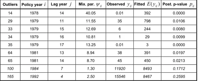
(20) Table 8 gives a summary of the parameters ψ ij , observed claims y ij and expected claims E ( y ij ) . The posterior p-values p ij is approximated using the following equation. rij < 0, ⎧ 2 F (ln( yij )), pij = ⎨ ⎩2[1 − F (ln( yij ))], rij ≥ 0, where F (⋅) is an approximated cumulative distribution function of the density function in (10) and μ ij is given by (6) to (9). All except observations 100 and 165, written in italic in Table 8, give negative residuals, rij = ln y ij − μ ij . The posterior p-values pij indicate that these extreme observations, except observations 100 and 165, are outliers. Table 8. Summary of the parameters ψ ij , observed values y ij , fitted values E ( y ij ) and the. posterior p-values p ij of the extreme observations. Outliers Policy year. i. Lag year. j. Mix. par. ψ ij. Observed. y ij. E ( y ij ). Fitted. Post. p-value. 14. 1978. 14. 40.05. 0.01. 392. 0.0000. 29. 1979. 11. 11.55. 35. 798. 0.0106. 33. 1979. 15. 12.69. 6. 244. 0.0080. 34. 1979. 16. 10.81. 1. 29. 0.0099. 35. 1979. 17. 13.25. 0.01. 3. 0.0000. 64. 1981. 13. 8.94. 38. 391. 0.0197. 65. 1981. 14. 8.70. 45. 450. 0.0213. 100. 1984. 7. 1.30. 11920. 8493. 0.1712. 165. 1992. 4. 2.50. 15546. 8467. 0.2595. pij. 6.4 Comparison with chain ladder method. The chosen model produces more accurate prediction of claims than the popular chain ladder method which indirectly estimates the incremental loss y ij by projecting the cumulative loss S ij Sîj = Sî , j −1 × f j ,. i = 2, K, n, j = n − i + 2, K, n. j. where S ij = ∑ y ij and Sî ,n+1−i = S i ,n+1−i using the projective factors k =1. fj. ∑ = ∑. n +1− j. i =1 n +1− j. i =1. S ij. S i , j −1. , j = 2,K, n .. The prediction of S ij on higher lag years, which is further away from the latest known claim amount requires the product of more projection factors and hence becomes less reliable as less data are available. We predict S ij in the upper triangle of Table 2 using only one year ahead projective factor so that Sˆ ij = S i , j −1 × f j ,. 2 ≤ j ≤ n − i +1. and Sˆ i1 = S i1 . We project S ij in the lower triangle by - 19 -.

(21) Sˆ ij = S i ,n −i +1 × ∏ kj = n −i + 2 f k , i = 2, K,18,. j > n − i +1.. The predicted and projected claims are reported in Table 9. Note that there are some negative values. They refer to predicted and projected claims which are very close to zero. The MSE for the predicted claims using the chain ladder method is 3,908,069 which is much larger than 1,584,478 for the chosen model. Moreover Figure 8 reveals that the predicted claims using the chosen model (black points) are closer to the observed claims than those using the chain ladder method (grey points). Thus the GT model provides more reliable prediction of loss reserves. Accurate prediction of loss reserves is very important to insurance companies since the levels of loss reserves have a dramatic impact on the profitability and solvency of insurance companies. Table 9. Run-off triangle of predicted and projected levels of claims using the chain ladder method.. 7. Conclusion. In this paper, log-linear models with three different forms of mean function are used to model loss reserves. For the data set analyzed, the GT error distribution performs better than the normal and other well-know heavy-tailed error distributions such as Student-t and EP distributions. Meanwhile, the time-recursive state space model with threshold in 1984 provides the best fit to the data. Prediction and projection of loss reserves are based on Bayesian approach. Expressing the GT distribution into the uniform scale mixtures form makes Gibbs sampler more efficient and enables outlier diagnostics using the scale mixture mixing parameters. Model selection relies on the Deviance information criterion. Comparing with the popular chain ladder method, the chosen GT model is shown to provide more accurate predicted claims. The chosen model is then used to project outstanding claims of the lower triangle in Table 2. As the log-linear model is more sensitive to low values than large values, the residuals for the data set analyzed are negatively skewed. To allow for a skewed error distribution, one may consider the skewed heavy-tailed distributions including the skewed-t distribution or the scale mixtures of beta distribution. Further investigation into the skewed error distributions will surely improve the modeling of loss reserve data.. - 20 -.

(22) Acknowledgement. The authors would like to thank Deborah Street and anonymous referees for very constructive comments, Connie P.Y. Lam for calculating the DICs and Wai-Yin Wan for running some WinBUGS programs. The second author is supported by an ECR grant of the University of Technology Sydney, Australia. Reference. Akaike, H., “A new look at the statistical model identification”, IEEE Transactions on Automatic Control, 19, 716–723, 1974. Arslan, O. and Genc, A.I., “Robust location and scale estimation based on the univariate generalized t (GT) distribution”, Communications in Statistics: Theory and Methods, 32, 1505-1525, 2003. Box, G.E.P. and Tiao, G.C., “A further look at robustness via Bayes' theorem”, Biometrika, 49, 419-432, 1962. Butler R.J., McDonald B.J., Nelson R.D., and White S.B., “Robust and Partially Adaptive Estimation of Regression Models”, MIT Press, 72, 321-327, 1990. Choy, S.T.B. and Chan, C.M., “Scale mixtures distributions in insurance applications”, ASTIN Bulletin, 33, 93-104, 2003. Choy, S.T.B. and Smith, A.F.M., “Hierarchical models with scale mixtures of normal distribution”, TEST, 6, 205-221, 1997. De Alba, E., “Bayesian estimation of outstanding claim reserves”, North American Actuarial Journal, October 2002. De Jong, P. and Zehnwirth, B., “Claims reserving state space models and Kalman filter”, The Journal of the Institute of Actuaries, 110, 157-181, 1983. Damien, P., Wakefield, J. and Walker, S., “Gibbs sampling for Bayesian non-Conjugate and hierarchical models by using auxiliary variables”, Journal of the Royal Statistical Society, Series B, 61, 331-344, 1999. Gelfand, A.E. and Smith A.F.M., “Sampling-based approaches to calculating marginal densities”, Journal of American Statistical Association, 85, 398-409, 1990. Geman, S. and Geman, D., “Stochastic relaxation, Gibbs distributions and the Bayesian restoration of images”, IEEE Transactions on Pattern Analysis and Machine Intelligence, 6, 721-741, 1984. Gelman, A., Carlin, J.B., Stern, H.S., and Rubin, D.B., Bayesian Data Analysis, 2nd edition, Chapman & Hall/CRC, 182–184, 2004. Gilks, W.R., Richardson, S. and Spiegelhalter, D.J., “Markov chain Monte Carlo in practice”, Boca Raton, Fla.: Chapman and Hall, 1998.. - 21 -.

(23) Green, P.J., “Reversible jump Markoc chain Monte Carlo computation and Bayesian model determination”, Biometrika, 82, 711-732, 1995. Hager, H.W. and Bain, L.J., “Inferential procedures for the generalized gamma distribution”, Journal of the American Statistical Association, 65, 1601-1609, 1970. Hastings, W.K., “Monte Carlo sampling methods using Markov Chains and their applications”, Biometrika, 57, 97-10, 1970. Hazan, A. and Makov, U.E., “A switching regression model for loss reserves”, Technical report TR24, 2001. Makov, U.E., “Perspective applications of Bayesian methods in actuarial science: a perspective”, North American Actuarial Journal, 2001. McDonald, J.B. and Butler, R.J., “Some generalized mixture distributions with an application to unemployment duration”, Review of Economics and Statistics, 69, 232-240, 1987. McDonald, J.B. and Newey, W.K., “Partially adaptive estimation of regression models via the generalized t distribution”, Economic Theory, 4, 428-457, 1988. Metropolis, N., Rosenbluth, A.W., Rosenbluth, M.N. and Teller, A.H., “Equations of State calculations by fast computing machines”, Journal of Chemical Physics, 21, 1087-1091, 1953. Ntzoufras, I. and Dellaportas P., “Bayesian modeling of outstanding liabilities incorporating claim count uncertainty”, North American Actuarial Journal, 6, 113-128, 2002. Ntzoufras, I., Katsis, A. and Karlis, D., “Bayesian assessment of the distribution of insurance claim counts using reversible jump MCMC”, North American Actuarial Journal, 9, 90-108, 2005. Renshaw, A.E., “Chain ladder and interactive modeling”, The Journal of the Institute of Actuaries, 116, 559-587, 1989. Renshaw, A.E., and Verrall, R.J., “A stochastic model underlying the chain-ladder technique”, British Actuarial Journal, 4, 903-926, 1998. Schwarz, G., “Estimating the dimension of a model”, Annals of Statistics 6(2), 461-464, 1978. Scollnik, D.P.M., “On the analysis of truncated generalized Poisson distribution using a Bayesian method”, ASTIN Bulletin, 28, 135-152, 1998. Scollnik, D.P.M., “Actuarial modeling with MCMC and BUGS”, North American Actuarial Journal, 5, 96-124, 2001. Scollnik, D.P.M., “Implementation of four models for outstanding liabilities in WinBUGS: A discussion of a paper by Ntzoufras and Dellaportas”, North American Actuarial Journal, 6, 128-136, 2002. - 22 -.

(24) Spiegelhalter, D., Thomas, A., Best, N.G. and Lunn, D., “Bayesian inference using Gibbs sampling for Window version (WinBUGS)”, Version 1.4.1, MRC Biostatistics Unit, Institute of Public health, Cambridge, UK. (www.mrc-bsu.cam.ac.uk/bugs/welcome.shtml), 2004. Spiegelhalter, D., Best, N.G., Carlin, B.P. and van der Linde, A., “Bayesian measures of model complexity and fit”, Journal of the Royal Statistical Society, Series B, 64, 583-639, 2002. Verrall, R.J., “State space representation of the chain ladder linear model”, The Journal of Institute of Actuaries, 116, 589-610, 1989. Verrall, R.J., “Chain ladder and maximum likelihood”, The Journal of Institute of Actuaries, 118, 489-499, 1991. Verrall, R.J., “A method of modeling varying-off evolutions in claims reserving”, ASTIN Bulletin, 24, 325-332, 1994. Verrall, R.J., “Claims reserving and generalized additive models”, The Journal of Institute of Actuaries, 19, 31-43, 1996. Verrall, R.J., “A Bayesian generalized linear model for the Bornhuetter-Ferguson method of claims reserving”, North American Actuarial Journal, 8, 67-89, 2004. Walker, S. G. and Gutiérrez-Peña, E., “Robustifying Bayesian procedures”, In: Bayesian Statistics 6. Oxford, New York, 685-710, 1999.. - 23 -.

(25) Appendix A WinBUGS command codes for M1 to M4 M1 log-ANOVA model model { for( i in 1 : N ) { z[i] <- log(y[i]) ub[i] <- pow(abs(z[i]-mu[i]),p)*pow(s[i],b)/(q*pow(sigma,p)) u[i] ~ dgamma(a,1)I(ub[i],1000) s[i] ~ gen.gamma(q,1, b) z[i] ~ dunif(lower[i],upper[i]) lower[i] <- mu[i]-sigma*pow(q,1/p)*pow(s[i],-1/2)*pow(u[i],1/p) upper[i] <- mu[i]+sigma*pow(q,1/p)*pow(s[i],-1/2)*pow(u[i],1/p) mu[i] <- mu0+alpha[row[i]]+beta[col[i]] } for (j in 2:18){ alpha[j] ~ dnorm(0, 0.01) beta[j]~ dnorm(0, 0.01) } alpha[1]<- 0-sum(alpha[2:18]) beta[1]<- 0-sum(beta[2:18]) mu0 ~ dnorm(0, 0.001) tau2 ~ dgamma(0.001,0.001) sigma2 <- 1/tau2 sigma <- pow(sigma2,0.5) p ~ dgamma(0.001,0.001) # when p is random #p <- 2 # when p is fixed at 2 say q ~ dgamma(0.001,0.001) # when q is random #q <- 2 # when q is fixed at 2 say a <- 1+1/p b <- p/2 }. M2 log-ANCOVA model model { for( i in 1 : N ) { z[i] <- log(y[i]) ub[i] <- pow(abs(z[i]-mu[i]),p)*pow(s[i],b)/(q*pow(sigma,p)) u[i] ~ dgamma(a,1)I(ub[i],1000) s[i] ~ gen.gamma(q,1, b) z[i] ~ dunif(lower[i],upper[i]) lower[i] <- mu[i]-sigma*pow(q,1/p)*pow(s[i],-1/2)*pow(u[i],1/p) upper[i] <- mu[i]+sigma*pow(q,1/p)*pow(s[i],-1/2)*pow(u[i],1/p) mu[i] <- mu0+alpha*row[i]+beta[col[i]] } for (j in 2:18){ beta[j]~ dnorm(0, 0.01) } beta[1]<- 0-sum(beta[2:18]) alpha ~ dnorm(0, 0.01) mu0 ~ dnorm(0, 0.001) tau2 ~ dgamma(0.001,0.001) sigma2 <- 1/tau2 sigma <- pow(sigma2,0.5) p ~ dgamma(0.001,0.001) # when p is random #p <- 2 # when p is fixed at 2 say q ~ dgamma(0.001,0.001) # when q is random #q <- 2 # when q is fixed at 2 say a <- 1+1/p b <- p/2 }. - 24 -.

(26) M3 State space model model { for( i in 1 : N ) { z[i] <- log(y[i]) ub[i] <- pow(abs(z[i]-mu[i]),p)*pow(s[i],b)/(q*pow(sigma,p)) u[i] ~ dgamma(a,1)I(ub[i],1000) s[i] ~ gen.gamma(q,1, b)I(0.01,1000) z[i] ~ dunif(lower[i],upper[i]) lower[i] <- mu[i]-sigma*pow(q,1/p)*pow(s[i],-1/2)*pow(u[i],1/p) upper[i] <- mu[i]+sigma*pow(q,1/p)*pow(s[i],-1/2)*pow(u[i],1/p) mu[i] <- mu0+alpha[row[i]]+beta[row[i],col[i]] } for (i in 1:18) { beta[i,1] <- 0 } for (j in 2:18) { beta[1,j] ~ dnorm(0, 0.01) } for (i in 2:18) { for (j in 2:18) { beta[i,j] <- beta[i-1,j]+v[i] } alpha[i] <- alpha[i-1]+h[i] v[i] ~ dnorm(0, tau2v) h[i] ~ dnorm(0, tau2h) } alpha[1] <- 0 mu0 ~ dnorm(0, 0.001) tau2 ~ dgamma(0.001,0.001) tau2v ~ dgamma(0.001,0.001) tau2h ~ dgamma(0.001,0.001) sigma2 <- 1/tau2 sigma2v <- 1/tau2v sigma2h <- 1/tau2h sigma <- pow(sigma2,0.5) p ~ dgamma(0.001,0.001) # when p is random #p <- 2 # when p is fixed at 2 say. M4 Threshold SS model model { # trend 1 for( i in 1 : N1-1 ) { z[i] <- log(y[i]) ub[i] <- pow(abs(z[i]-mu[i]),p)*pow(s[i],b)/(q*pow(sigma,p)) u[i] ~ dgamma(a,1)I(ub[i],1000) s[i] ~ gen.gamma(q,1, b)I(0.01,1000) z[i] ~ dunif(lower[i],upper[i]) lower[i] <- mu[i]-sigma*pow(q,1/p)*pow(s[i],-1/2)*pow(u[i],1/p) upper[i] <- mu[i]+sigma*pow(q,1/p)*pow(s[i],-1/2)*pow(u[i],1/p) mu[i] <- mu01+alpha1[row[i]]+beta1[col[i]] } for (i in 1:T-1) { beta1[i,1] <- 0 } for (j in 2:18) { beta1[1,j] ~ dnorm(0, 0.01). q ~ dgamma(0.001,0.001) #q <- 2 a <- 1+1/p b <- p/2 }. lower[i] <- mu[i]-sigma*pow(q,1/p)*pow(s[i],-1/2)*pow(u[i],1/p) upper[i] <- mu[i]+sigma*pow(q,1/p)*pow(s[i],-1/2)*pow(u[i],1/p) mu[i] <- mu02+alpha2[row[i]-T+1]+beta2[col[i]] } for (i in 1:18-T+1) { beta2[i,1] <- 0 } for (j in 2:18-T+1) { beta2[1,j] ~ dnorm(0, 0.01) beta2r1[j] <- beta2[1,j] } for (i in 2:18-T+1) { for (j in 2:18-T+1) { } beta2[i,j] <- beta2[i-1,j]+v2[i] } alpha2[i] <- alpha2[i-1]+h2[i]. # when q is random # when q is fixed at 2 say. beta1r1[j] <- beta1[1,j] } for (i in 2:T-1) { for (j in 2:18) { beta1[i,j] <- beta1[i-1,j]+v1[i] } alpha1[i] <- alpha1[i-1]+h1[i] v1[i] ~ dnorm(0, tau2v1) h1[i] ~ dnorm(0, tau2h1) } alpha1[1] <- 0 beta1r1[1] <- 0 # trend 2 for( i in N1 : N ) { z[i] <- log(y[i]) ub[i] <- pow(abs(z[i]-mu[i]),p)*pow(s[i],b)/(q*pow(sigma,p)) u[i] ~ dgamma(a,1)I(ub[i],1000) s[i] ~ gen.gamma(q,1, b)I(0.01,1000) z[i] ~ dunif(lower[i],upper[i]). - 25 -.

(27) v2[i] ~ dnorm(0, tau2v2) h2[i] ~ dnorm(0, tau2h2) } alpha2[1] <- 0 Beta2r1[1] <- 0 # end trend 2 mu01 ~ dnorm(0, 0.001) mu02 ~ dnorm(0, 0.001) tau2 ~ dgamma(0.001,0.001) tau2v1 ~ dgamma(0.001,0.001) tau2h1 ~ dgamma(0.001,0.001) tau2v2 ~ dgamma(0.001,0.001) tau2h2 ~ dgamma(0.001,0.001) sigma2 <- 1/tau2 sigma2v1 <- 1/tau2v1 sigma2h1 <- 1/tau2h1 sigma2v2 <- 1/tau2v2 sigma2h2 <- 1/tau2h2 sigma2v1 <- 1/tau2v1 sigma <- pow(sigma2,0.5) p ~ dgamma(0.001,0.001) # when p is random #p <- 2 # when p is fixed at 2 say q ~ dgamma(0.001,0.001) # when q is random #q <- 2 # when q is fixed at 2 say a <- 1+1/p b <- p/2 }. ] [ l o c ] [ w o r ] [ y. Remark: 1. Data are entered using the following format: 3323 8332 …. 1 1 1 2. 2827 END. 18. 1. 2. Values for some constants are: list(N=171, T=7, N1=94) list(N=171). # threshold model # simple model. For T=5,6,7,8,9, N1=67,81,94,106,117 respectively. 3. Starting values for the parameters are: 0.1 for mu01, mu02, 0.000001 for tau2, tau2h1, tau2v1, tau2h1, tau2v1, 0 for h1, h2, v1 and v2, all 1 for u and all 2 for s) for the threshold SS model. 4. Model parameters for the threshold SS model which are stored for calculation include: mu01,mu02,v1,h1,v2,h2,alpha1,alpha2,beta1r1,beta2r1,sigma2h1,sigma2v1,sigma2h2,sigma2v2,u,s,p,q,sigma2. Note that beta1r1 and beta2r1 store the beta in the first row for trend 1 and 2 respectively. The. lengths of alpha1,h1,v1 are T-1, the length of beta1r1 is 18 and alpha1[1]= beta1r1[1]=h1[1]=v1[1]=0. The lengths of alpha2, beta2,h2,v2 are 18-T+1 and alpha2[1]= beta2r1[1]=h2[1]=v2[1]=0. β ij can be calculated using (7) for each k, beta1r1, beta2r1, v1 and v2.. - 26 -.

(28) Appendix B Figure 9(a) – (e) Various density functions for the GT distribution. G T distributions w hen q = 2. G T distributions w hen q = 0.5 p= p= p= p= p= p= p= p=. 0.25 0.5 1 2 5 15 50 100. p= p= p= p= p= p= p= p=. 0. 0. -3. -2. -1. 0. 1. 2. -3. 3. G T distributions w hen q = 1. -2. -1. 0. 1. 2. p= p= p= p= p= p= p= p=. p=1 p=2 p=5 p = 15 p = 50 p = 100. -1. 0.25 0.5 1 2 5 15 50 100. 0. 0. -2. 3. G T distributions when q = 50 p = 0.25 p = 0.5. -3. 0.25 0.5 1 2 5 15 50 100. 0. 1. 2. -3. 3. -2. -1. 0. 1. 2. 3. G T distributions w hen p = q p = q = 0.25 p = q = 0.5 p=q=1 p=q=2 p=q=5 p = q = 15 p = q = 50 p = q = 100. 0. -3. - 27 -. -2. -1. 0. 1. 2. 3.

(29)

No results found