Application and Development of
Computational Methods for
Ligand-Based Virtual Screening
Kumulative Dissertation
zur Erlangung des Doktorgrades (Dr. rer. nat.)
der Mathematisch-Naturwissenschaftlichen Fakultät
der Rheinischen Friedrich-Wilhelms-Universität Bonn
vorgelegt von
Kathrin Heikamp
aus Bonn
der Rheinischen Friedrich-Wilhelms-Universität Bonn
1. Gutachter: Univ.-Prof. Dr. rer. nat. Jürgen Bajorath
2. Gutachter: Univ.-Prof. Dr. rer. nat. Andreas Weber
Tag der Promotion: 11. April 2014
Abstract
The detection of novel active compounds that are able to modulate the bio-logical function of a target is the primary goal of drug discovery. Different screening methods are available to identify hit compounds having the desired bioactivity in a large collection of molecules. As a computational method, vir-tual screening (VS) is used to search compound libraries in silico and identify those compounds that are likely to exhibit a specific activity. Ligand-based virtual screening (LBVS) is a subdiscipline that uses the information of one or more known active compounds in order to identify new hit compounds. Differ-ent LBVS methods exist, e.g. similarity searching and support vector machines (SVMs). In order to enable the application of these computational approaches, compounds have to be described numerically. Fingerprints derived from the two-dimensional compound structure, called 2D fingerprints, are among the most popular molecular descriptors available.
This thesis covers the usage of 2D fingerprints in the context of LBVS. The first part focuses on a detailed analysis of 2D fingerprints. Their performance range against a wide range of pharmaceutical targets is globally estimated through fingerprint-based similarity searching. Additionally, mechanisms by which fin-gerprints are capable of detecting structurally diverse active compounds are identified. For this purpose, two different feature selection methods are applied to find those fingerprint features that are most relevant for the active com-pounds and distinguish them from other comcom-pounds. Then, 2D fingerprints are used in SVM calculations. The SVM methodology provides several opportuni-ties to include additional information about the compounds in order to direct LBVS search calculations. In a first step, a variant of the SVM approach is ap-plied to the multi-class prediction problem involving compounds that are active against several related targets. SVM linear combination is used to recover com-pounds with desired activity profiles and deprioritize comcom-pounds with other activities. Then, the SVM methodology is adopted for potency-directed VS. Compound potency is incorporated into the SVM approach through potency-oriented SVM linear combination and kernel function design to direct search calculations to the preferential detection of potent hit compounds. Next, SVM calculations are applied to address an intrinsic limitation of similarity-based
sets on the recall performance of SVM-based VS is analyzed and caveats are identified.
Acknowledgements
I would like to take the opportunity and thank the persons who accompanied me during the last years and contributed to the completion of this dissertation in many different ways.
First of all, I like to thank my supervisor Prof. Dr. Jürgen Bajorath for his in-valuable guidance, continuous support and encouragement throughout my PhD study. I also like to thank Prof. Dr. Andreas Weber for being the co-referent of my thesis.
I would like to express my gratitude to all my colleagues of the LSI research group for providing a helpful, friendly and interactive working atmosphere. There have been many joyful and funny moments, both inside and outside the BIT, that I will not forget. Furthermore, many thanks are given to Anne Mai Wassermann, Dagmar Stumpfe, Dilyana Dimova and Jenny Balfer for produc-tive and pleasant collaborations. I would like to thank Martin Vogt for being approachable for my questions at any time.
Moreover, special thanks are given to Dilyana Dimova for her encouragement and understanding, and for becoming a close friend during the last years. I would like to thank Dagmar Stumpfe for being a confidential person and her patient advices in scientific and personal questions. Furthermore, I like to thank Antonio de la Vega de León for his cheerfulness and his sense of humor.
Finally, I am grateful to my family and friends for their encouragement and support during the last years. Especially, I thank André Oeckerath for his reliable and invaluable support and motivation.
Contents
Introduction 1
Thesis outline 35
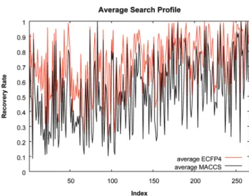
1 Large-scale similarity search profiling of ChEMBL compound
data sets 37
Introduction . . . 37 Publication . . . 39 Summary . . . 49
2 How do 2D fingerprints detect structurally diverse active com-pounds? Revealing compound subset-specific fingerprint
fea-tures through systematic selection 51
Introduction . . . 51 Publication . . . 53 Summary . . . 65
3 Prediction of compounds with closely related activity profiles using weighted support vector machine linear combinations 67
Introduction . . . 67 Publication . . . 69 Summary . . . 81
4 Potency-directed similarity searching using support vector
ma-chines 83
Introduction . . . 83 Publication . . . 85 Summary . . . 95
5 Prediction of activity cliffs using support vector machines 97
Introduction . . . 97 Publication . . . 99
machine-based virtual screening 113
Introduction . . . 113 Publication . . . 115 Summary . . . 123
List of abbreviations
1D One-dimensional
2D Two-dimensional
3D Three-dimensional
AUC Area under the ROC curve
ECFP Extended-connectivity fingerprint
FP Fingerprint
HTS High-throughput screening
IC50 Half maximal inhibitory concentration
Ki Inhibition dissociation constant
kNN k-nearest neighbors
LBVS Ligand-based virtual screening
LC Linear combination
MACCS Molecular ACCess System
ML Machine learning
MMP Matched molecular pair
MOE Molecular Operating Environment
QSAR Quantitative structure–activity relationship
ROC Receiver operating characteristic
SAR Structure-activity relationship
SBVS Structure-based virtual screening
SPP Similarity property principle
SVM Support vector machine
SVR Support vector regression
Tc Tanimoto coefficient
TGD Typed graph distance
TGT Typed graph triangle
Introduction
Drug discovery is concerned with the detection of small molecules that are ac-tive against a biological target and modulate its biological function. The whole process until a drug can be used as a medication for a specific disease requires several years and is very costly [1]. Furthermore, only a small proportion of candidate compounds is approved and brought to market [1, 2]. The drug dis-covery process involves several preclinical and clinical stages with numerous investigators involved. In the preclinical phase, the major stages include the identification and validation of novel drug targets, the identification of active compounds (so-called hits), and the transformation of hits to lead compounds that can be further optimized [2–4].
The major source of hits is high-throughput screening (HTS) [5, 6]. In HTS, a very large collection of compounds is tested for a biochemical or cellular effect [6]. Those compounds having a positive response in the screening are considered as hit compounds. In follow-up screens, these hits are analyzed con-cerning pharmacological and physicochemical properties and evaluated for their potential to become a lead compound [6]. In general, HTS data are of limited quality due to the presence of false-positive and false-negative activity measure-ments. The typically large number of false-positives makes subsequent control experiments necessary. False-negative measurements are often a consequence of limited purity and stability of test compounds or of too low concentrations in the screening assay [5, 7].
In order to compensate for such limitations, computational approaches have been developed. Among them, virtual screening (VS) was introduced as a com-putational, “time-efficient and cost-effective” [5] analog to HTS. In VS, a large compound library is screened in silico against a drug target of interest. Test
a specific activity and a reduced list of compounds is submitted to biological experiments [5, 7–9]. Although VS also suffers from false predictions, it was shown that VS often produces higher hit rates than HTS [9].
In general, HTS and VS are considered to be complementary screening meth-ods [5, 7]. Hence, the integration of computational and biological screening is considered in order to reduce the number of candidate compounds and thereby the costs of experimental testing [7, 10].
VS includes two different approaches: structure-based virtual screening (SBVS) [11, 12] and ligand-based virtual screening (LBVS) [10, 11, 13]. SBVS methods use the three-dimensional (3D) structure of a target in order to make assump-tions about the interacassump-tions between ligand and target. The most popular SBVS method is docking, where database compounds are docked into the 3D struc-ture of the target in order to predict the hypothetical binding modes. Then, a score is calculated that reflects the estimated binding affinity of the compound and serves as an indication which compounds should be tested [12, 14].
In contrast, LBVS makes use of ligand information only. The LBVS methods require one or more compounds with a specific activity to identify new hits. Conceptually, LBVS is based on the similarity property principle (SPP) formu-lated by Johnson and Maggiora in 1990 [15]. The principle states that “similar molecules should have similar biological properties (activity)”. Subdisciplines of LBVS methods include pharmacophore searching [16], shape comparison [17], similarity searching [18, 19], and machine learning [13]. In the following, sim-ilarity searching and an example of a machine learning method, the support vector machines, are discussed in more detail.
Similarity searching
Similarity searching is one of the most widely used LBVS approaches in drug discovery. One or multiple active compounds are used as reference compounds (or templates) to screen a large database of compounds with unknown activity. The database compounds are compared to the reference set and ranked in the order of decreasing similarity. According to the SPP, those compounds that
Similarity searching
are located at the top positions of the ranking most probably exhibit a similar bioactivity [19].
For similarity searching, three principal components have to be defined: (i) a molecular representation for the compounds, (ii) a coefficient for determining the similarity, and (iii) a search strategy [19, 20]. They are discussed in detail in the following.
Molecular representations
Molecular descriptors are used to numerically describe the molecular structure
and compound properties. There are many molecular descriptors of
differ-ent complexity available that capture differdiffer-ent levels of compound information [21]. In general, one can classify molecular descriptors as one-, two- or three-dimensional (1D, 2D, 3D) depending on the structure representation from which they are derived [7]. 1D descriptors are calculated from the molecular formula not considering atom connectivities. Examples of 1D descriptors are atom count and molecular weight. 2D descriptors are derived from the molecular graph and include topological descriptors as well as calculated descriptors approximating compound properties like logP. Molecular conformations are used to determine 3D descriptors. These descriptors comprise, e.g., volume or molecular surface [7].
The most popular molecular descriptors include molecular fingerprints (FPs) that are bit or integer string representations capturing structural features and physicochemical properties of compounds [22]. In binary fingerprints, each bit in the string encodes the presence or absence of a specific feature. If a specific feature is present in the molecule, the bit is set to ’1’; otherwise, it is set to ’0’. There are also non-binary count fingerprint versions where the bits are replaced with an integer indicating the frequency of the features. Integer-based fingerprints are derived when compound features are hashed.
In analogy to the molecular descriptors, one can distinguish 2D and 3D FPs based on the structure representation of the molecule [19]. Furthermore, dif-ferent types of fingerprints have been introduced that vary in the encoding of chemical information and how they are calculated. Hence, they capture
dif-Substructure FP H H 11 A 8 5 Ar H D 13 5 7 Pharmacophore FP Combinatorial FP 1. Layer c 2. Layer cc(c)C 3. Layer nc(N)c(C(=O)N)cn ...
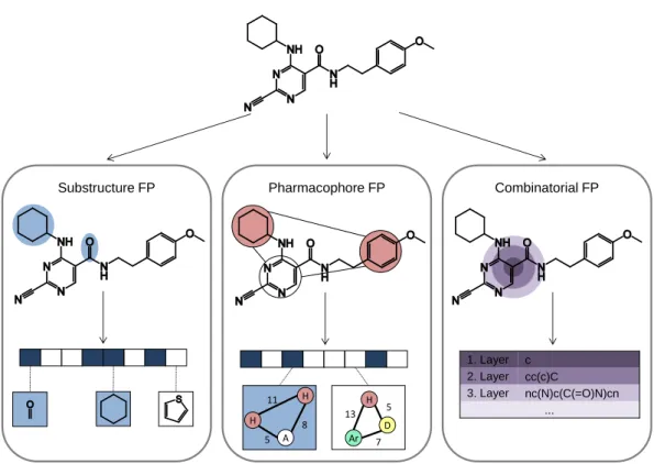
Figure 1: Fingerprint prototypes. Three different fingerprint designs are compared. (i) An exemplary keyed substructure FP is shown. Bit positions are set on (i.e., blue) if the corresponding substructure is present and set off otherwise (i.e., white). Two substructures, a carbonyl group and a ring, that account for two bits set are highlighted in the compound structure. (ii) In a pharmacophore FP, each bit accounts for one geometrical arrangement of atom types. Here, the threepoint pharmacophore pattern “hydrophobic hydrophobic -hydrogen bond acceptor” with the defined inter-feature distances is available in the structure and the according bit is set on. (iii) A combinatorial FP encoding local atom environments is illustrated. Around a central atom, here a carbon, three layers are created up to a diameter of four bonds. The resulting circular environments are hashed. The figure is adapted from [22].
include substructure-based fingerprints, pharmacophore fingerprints, and com-binatorial fingerprints like circular atom environments. These fingerprint types are compared in Figure 1 and discussed below.
Two popular substructure-based fingerprints are the Molecular ACCess Sys-tem (MACCS) structural keys [23] and the BCI fingerprint [24]. The publicly available version of MACCS contains 166 structural fragments and the BCI consists of 1,052 substructures. Both fingerprints are keyed fingerprints with a one-to-one mapping of each bit position to a structural fragment. Each bit in the fingerprint then accounts for the presence or absence of the according substructure.
Similarity searching
Pharmacophore fingerprints also belong to the class of keyed fingerprints. Each bit in the string encodes one geometrical arrangement of atom types. The pharmacophore fingerprint of a compound is derived by generating all possi-ble pharmacophore patterns of the compound. That means, in the first step atomic features (e.g. hydrogen bond donor or acceptor) are assigned to individ-ual atoms or groups of atoms. Then, all possible combinations of two to four atomic features and their inter-feature distances are determined. The Molec-ular Operating Environment (MOE) [25] contains several different 2D and 3D pharmacophore fingerprints. For example, the typed graph distance (TGD) and typed graph triangle (TGT) fingerprints consist of 420 and 1704 bit positions or pharmacophore patterns, respectively, which can be derived from the 2D molecular graph. Thereby, TGD encodes the distance of atomic features and TGT is a three-point pharmacophore encoding feature triangles.
In contrast, combinatorial fingerprints represent another concept as they do not have a predefined length. For example, the extended-connectivity fingerprints (ECFPs) [26] encode circular atom environments. Each non-hydrogen atom in the molecule is assigned to an atom code describing its mass, charge, element type, valence, and the number of neighboring atoms. Then, a local atom envi-ronment is created around each atom up to a specific bond depth. The resulting features are hashed to an integer and the final collection of integers forms the fingerprint. Hence, the size of ECFPs is dependent on the given compound. A comparable FP is MOLPRINT2D [27]. It also consists of molecule-specific atom environments. However, different atom encodings are used and the atom environments are encoded as strings of varying size.
Although 2D fingerprints have a lower information content than 3D molecular representations, screening calculations based on 3D descriptors do not princi-pally perform better than similarity searching using 2D fingerprints [28–30]. Important information about target-ligand interactions are implicitly encoded in 2D fingerprint representations [31]. In general, 2D fingerprints are simpler and more robust as they do not require an approximation of the bioactive com-pound conformation. Therefore, several studies focus on 2D FPs only [20]. Among the 2D FPs, the ECFPs showed the best screening performance in sev-eral studies [32, 33].
Similarity coefficients
The similarity between two compounds is typically assessed by a fingerprint comparison. A similarity measure is used to quantify the compound similarity by determining the overlap between the fingerprint strings. The most frequently used similarity measure for binary fingerprints is the Tanimoto (or Jaccard) coefficient (Tc) [18], that is a function Tc : {0,1}n× {0,1}n → [0,1]. For two molecular fingerprints A and B, the Tc is defined as
Tc(A, B) = c
a+b−c (1)
where a and b are the number of the bits set on in the fingerprints A and B, respectively, and c corresponds to the number of bits set in both fingerprints. It follows that the Tc compares the intersection of fingerprint features with the union of all features present in two compound fingerprints. The Tc values range from zero to one, where zero corresponds to minimal fingerprint similarity and one is the maximal similarity.
The Tc can also be applied to non-binary fingerprints. Then, the Tc calculates the fingerprint overlap by
Tc(A, B) = Pn i=1aibi Pn i=1(a 2 i +b2i −aibi) (2)
Here, the fingerprints have the formA= (a1, a2, . . . , an)andB = (b1, b2, . . . , bn)
with a length of n. The variables ai and bi represent the ith position in the
fingerprints A and B, respectively, and aibi is their product. The non-binary
Tc has a value range of -0.333 to 1 [18].
Other popular similarity coefficients used in similarity searching include the Tversky coefficient [34], the Forbes coefficient [35], and the Russel-Rao coeffi-cient [35].
Search strategies
Although similarity searching can be applied with only one reference compound, using multiple active compounds usually improves the search performance [36].
Support vector machines
There exist different strategies how to make use of the information provided by the multiple references. In general, we can distinguish the two categories data fusion and fingerprint modifications [19].
In the first case, a fusion rule is applied on the similarity values or compound
ranks after multiple search calculations have been performed. The k-nearest
neighbors (kNN) search method [37, 38] is widely applied in combination with Tc similarity values. In kNN similarity searching, the similarity between all reference compounds to a database compound is individually calculated. The final similarity score for the current database molecule is then the averaged
similarity of the k most similar reference compounds. This value is used for
ranking. For example, in 10NN searching using Tc similarity the database score is the average of the 10 highest Tc values derived from at least 10 reference com-pounds. In 1NN search calculations, the maximal similarity yields the database score.
In contrast, fingerprint modification techniques alter the fingerprint represen-tation that is used for searching. In the centroid method, multiple reference compounds are combined by averaging over each bit position in the reference fingerprints [37]. The generated non-binary fingerprint is then used for screen-ing calculations. Furthermore, a consensus fscreen-ingerprint [39] can be constructed where individual bit positions are set on if the bit frequency in the reference compounds reaches a predefined threshold. In addition, other “fingerprint en-gineering” methods have been introduced to improve search performance using multiple references [40–43].
Support vector machines
Over the last years, machine learning (ML) methods have become increasingly important to address complex tasks in drug discovery [13]. The general aim of ML is the derivation of a computational model that learns labels from pat-terns in data, here in compound data. The models can then be applied for property predictions and classification of new, previously not considered com-pounds. Analogous to similarity searching, the models are also used to rank
support vector machines (SVMs) are one of the most popular techniques. They have become increasingly popular during the 1990s based on the work of Vap-nik and Cortes [44]. The basic idea of SVMs is the generation of a hyperplane in a high-dimensional space to derive a separation of objects from two classes. Thereby, a key feature of the SVM approach is the attempt to simultaneously address two conflicting objectives: (i) minimization of errors on training data and (ii) reduction of model complexity in order to avoid overfitting. The result balancing these objectives is a model with high generalization potential.
SVM classification and ranking
SVMs are a supervised machine learning method that makes use of annotated training examples [45–47]. Originally, the SVM approach was developed to
solve binary classification problems. During learning, SVM uses a set of n
training data {xi, yi} (i = 1, . . . , n) with xi ∈ X (e.g. Rd) being a feature
vector representation and yi ∈ {−1,1} the class label (negative or positive) of
the training compoundi. The SVM derives a hyperplaneH that best separates
positive from negative instances:
H ={x| hw,xi+b= 0}, (3)
where h·,·i is a scalar product,w the normal vector of the hyperplane and b a scalar.
For linearly separable training data, there exist an infinite number of hyper-planes that correctly classify the data. The optimal hyperplane chosen by the SVM algorithm is the hyperplane that maximizes the distance from the closest training instances to the hyperplane (called margin). The optimal, so-called
maximum margin hyperplane minimizes the “structural risk” of overfitting and
enhances the generalization of the classification model. The distance from the hyperplane H to the nearest training instances from the positive and negative class is 1/kwk each. Hence, maximizing the distance 1/kwk or,
minimiza-Support vector machines
tion problem is a constrained quadratic programming optimization problem and is formulated as minimize: w,b 1 2kwk 2 (4) subject to: yi(hxi,wi+b)≥1 ∀i
The inequality constraints are defined in order to ensure correct classification of all training examples, which is possible because of the assumed linear sepa-rability of the training data.
In case the training data are not linearly separable, the minimization problem has no solution. Then, so-called slack variables ξi ≥ 0 can be introduced and
a soft-margin separating hyperplane is derived. The slack variables relax the constraints defined in equation (4) and allow some training data to be located within the margin or even on the incorrect side of the hyperplane. The value of the slack variablesξicorrelates with the degree of mispositioning of the training
compound i. The minimization problem is reformulated as
minimize: w,b 1 2kwk 2 +CX i ξi (5)
subject to: yi(hxi,wi+b)≥1−ξi with ξi ≥0 ∀i
In this formulation, the constant C > 0 is introduced to penalize large slack variables. IfC is small, largeξi are allowed and a less complex model is learned
tolerating many errors. However, if C is large, ξi has to be small in the
mini-mization and a complex model is learned avoiding large errors. The parameter C can be considered as a trade-off between the size of the margin and the best fit of the classifier to the training data.
In order to solve this optimization problem, Lagrange multipliers αi are used
to reformulate the problem from the primal to a dual form: maximize: α LD = X i αi− 1 2 X i,j αiαjyiyjhxi,xji (6) subject to: X i αiyi = 0 with 0≤αi ≤C ∀i
H margin Data points positive class negative class hyperplane H support vector hyperplane parallel to H Hyperplanes
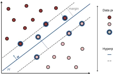
Figure 2: SVM classification. In a binary classification problem, the maximum margin hyperplane H separates two classes (dark and light red dots, respectively). The optimal hyperplane is shown as a blue solid line. Those data points that determine the hyperplane, the support vectors, are encircled in blue. They either lie on the edge of the margin (i.e. on the hyperplanes parallel toH), within the margin, or on the incorrect side of the hyperplane. Misclassified data points obtain values of the slack variables that correlate with the distance to the margin, as illustrated by the dotted lines. The figure is adapted from [48].
This optimization problem is convex and hence has a solution that is the global optimum. Solving the Lagrangian dual formulation results in the normal vector
w = P
iαiyixi with non-negative αi. Those training instances that are
asso-ciated with factors αi greater than zero are the so-called support vectors and
solely determine the position of the hyperplane. These data points lie on the edge, within the margin or even on the incorrect side of the hyperplane. Hence, the generation of the hyperplane only depends on some training examples and not on the dimension of the input space, which allows calculations in a higher dimensional space. A schematic illustration of an SVM classification problem is shown in Figure 2.
Once the normal vectorwhas been calculated, the scalarb can be derived from any support vector. Then, the final decision function (or separation rule) for the classification can be formulated as
f(x) = sgn X
i
αiyihxi,xi+b
!
(7)
The signum function sgn determines the sign of the prediction value for a test instancex. Geometrically, this is the side of the hyperplane onto which the test
Support vector machines
example falls. This means that test points (i.e. compounds) with f(x) = 1 are assigned to the positive class and those with f(x) =−1 to the negative class. In order to adapt the SVM approach for VS and allow ranking of test com-pounds, the decision function is transformed into a ranking function. This is obtained by removing the signum function from the decision function, thus generating a real value for each test example, i.e.
g(x) =X
i
αiyihxi,xi+b (8)
Then, test compounds are ranked from the highest to the lowest value. This corresponds to a ranking from the most distant data point on the positive half space to the most distant point on the negative half space [49].
SVM for regression
The SVM approach can also be used to generate real values by estimating a regression function [45, 47, 50]. SVM for regression, also called support vector regression (SVR), has a methodological basis comparable to SVM classification seeking for margin maximization. The training instances for SVR are a set of the form{xi, yi}withxi being a feature representation from input spaceX and
yi ∈ R a real value for each training data point i. SVR derives a regression
function of the form f(x) = hw,xi+b, mapping training data xi as close as
possible to their real value yi with a maximum deviation of . Hence, the
SVR approach tolerates errors less than , but deviations beyond this value
are penalized. Therefore, SVR is also termed -SVR [50]. Similar to SVM
classification, the optimization problem is formulated as minimize: w,b 1 2kwk 2 +CX i (ξi+ξi∗) (9) subject to: yi− hw,xii −b≤+ξi ∀i hw,xii+b−yi ≤+ξi∗ ∀i with ξ, ξ∗ ≥0
ε-tube Data points hyperplane H support vector hyperplane parallel to H Hyperplanes training data
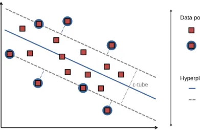
Figure 3: SVM for regression. In SVR, a regression line is fitted to the training data (shown as red squares). The regression function is shown as a solid blue line. It depends on those data points that lie on the edge of the-tube or outside (shown with dotted lines). These data points are the support vectors and are highlighted by blue circles. All other data points are fitted with sufficient precision and lie within the tube. The figure is adapted from [48].
In SVR, two sets of non-negative slack variables are required to account for positive and negative deviations of the predicted regression value to the true output value. Again, the constantC > 0is used to penalize large slack variables, i.e. deviations from the so-called-tube. After solving the optimization problem using Lagrangian reformulation, the final regression function is defined as
f(x) = X
i
(αi−α∗i)hxi,xi+b (10)
Those training data points having either αi > 0 or α∗i > 0 are the support
vectors. There are two types of support vectors. In the first case, the support vectors lie exactly on the boundary of the -tube. They have either0< αi < C
or 0 < α∗i < C and are used to derive the parameter b. The other support vectors fall outside of the tube and have αi =C or α∗i =C. All other training
data points have both αi =α∗i = 0 and are fitted with sufficient precision [47].
Support vector machines
input space high-dimensional space
mapping Φ
input space Figure 4: Kernel trick. On the left, data points from two different classes are shown as dark and light red points, respectively. A linear separation of the two classes is not possible in the 2D reference space. However, using a kernel function that implicitly transforms the data into a higher dimensional space (here, a 3D reference space) enables a linear separation. The linear decision function in the 3D space corresponds to an ellipse decision boundary in the input space. The figure is adapted from [48].
Kernel functions
In some cases, a linear separation of training data might not be feasible in
space X. In order to allow nonlinear separation rules, the so-called kernel
trick [51] can be applied to replace the standard scalar producth·,·iby a kernel functionK(·,·). The kernel transfers the calculations of the scalar product into a higher dimensional spaceHby a nonlinear transformationΦwithout explicitly
calculating the mapping Φ : X → H. The kernel function K : X × X → R
is defined by the scalar product between transformed objects xi and xj ∈ X
as K(xi,xj) = hΦ(xi),Φ(xj)i. The kernel function can be considered as a
specialized similarity measure between two arbitrary data points. Because the embedding function Φdoes not have to be known, only a valid kernel has to be defined. A valid kernel has to meet two conditions: it must be (i) symmetric, i.e. K(xi,xj) = K(xj,xi) for all xi ∈ X, and (ii) positive semi-definite, i.e.
the kernel (or Gram) matrix K = (K(xi,xj))ij is positive semi-definite for
x1, . . . ,xn ∈ X [47, 52, 53]. This requirement is met if for allc∈RncTKc≥0, i.e. Khas only non-negative eigenvalues. Here, the condition of positive semi-definiteness guarantees that the optimization problem remains convex.
The kernel trick can be used in SVM classification, ranking and regression. It replaces the standard scalar product of training and test instances in the
decision function. Then, the linear model in the new space H corresponds to
Popular kernel functions that are used in SVM calculations include, e.g., the linear kernel that corresponds to the standard scalar product:
Klinear(xi,xj) =hxi,xji (11)
The Gaussian kernel, also known as the radial basis function kernel, is defined as
KGaussian(xi,xj) =exp −γkxi−xjk2
(12) The Gaussian kernel depends on the choice of the inverse-width parameter γ > 0. Small values of γ result in a smooth decision boundary. However, a large γ increases the flexibility of the decision boundary by incorporating more support vectors raising the risk of overfitting [49, 54].
Finally, the polynomial kernel is given by
Kpolynomial(xi,xj) = (hxi,xji+ 1)d (13)
In the polynomial kernel, the parameter d∈N determines its degree. Thereby, a kernel with d = 1 is the linear kernel with offset 1. Higher values of d result in more flexible decision boundaries [54].
A useful property of kernel functions is that new kernel functions can be built by applying mathematical operations such as multiplication and addition to original kernels [55]. This also allows the design of kernel functions that can be applied on different data types.
Kernel functions in drug discovery
There are several kernel functions available that have been designed to operate on compounds and other bioactivity data. These include compound kernels that accept different compound representations as input and compare diverse properties of molecules. Other kernel functions use multiplication of kernels in order to derive a similarity measure on combined compound-target data.
Support vector machines
Compound kernels
Compounds are typically represented as graphs where atoms are shown as la-beled vertices and bonds as lala-beled edges. Several kernel functions have been created to operate on this graph-structured data (see below). These graph kernels allow the comparison of compounds for determining their similarity without ever computing or storing a feature vector representation of the com-pounds. Gärtner et al. [56] and Kashima et al. [57] introduced graph kernels that measure the overall similarity between two molecular graphs by detecting and counting common walks of equal label sequences in two labeled graphs. In the first case, the kernel is based on the direct graph product [56]. The second kernel belongs to the class of marginalized kernels and uses Markov random walks on the underlying graph structures [57]. In addition to these global graph kernels, there are kernels capturing the local similarity between two graphs [58]. Furthermore, extensions to graph kernels have been introduced [59]. The first extension is a relabeling of vertices so that the new atom labels include information about the topological environment. The second extension covers a modification of the random walk model proposed in [57] in order to prevent irregular loops along an edge, so-called totters.
Although these extensions aim at reducing the computational expense and im-proving prediction accuracy, graph kernels still are computationally complex and require parameter determination. In order to circumvent these limitations, another direction of kernel design consists of transforming the compound graphs into vectors using molecular descriptors. Ralaivola et al. [60] introduced several new kernel functions that are applied on molecular fingerprints or compound descriptor vectors and are thus computed more efficiently. Among others, the Tanimoto kernel is mentioned that is defined in accordance with the popular Tanimoto coefficient (2) as
KTanimoto(xi,xj) =
hxi,xji
hxi,xii+hxj,xji − hxi,xji
(14)
The Tanimoto kernel is parameter-free. Selecting different compound represen-tations allows the comparison of different compound properties of interest. Furthermore, kernel functions have been developed that consider the 3D
struc-three-point pharmacophores composed of three atoms, i.e., atom triangles, in 3D space. It can be decomposed into two separate kernels where the first ker-nel determines the similarity between the atoms and the second kerker-nel assesses the spatial similarity, i.e., the relative locations of the triangle atoms. The similarity between two molecules is finally assessed by summing up the pair-wise similarities between all possible pharmacophores in the compounds. The pharmacophore kernel was shown to outperform fingerprint representations of pharmacophores in SVM calculations [61].
Azencott et al. [62] discussed various classes of kernels derived from different levels of molecular representations ranging from 1D to 4D. Molecules were rep-resented as SMILES (1D), bond graphs (2D) or by their 3D atom coordinates. Using the 3D compound structure, additional kernel functions were obtained, e.g. a 2.5D surface kernel and diverse 3D kernels based on Delaunay tetra-hedrization, atomic coordinates or pharmacophores. Furthermore, they intro-duced an additional dimension for kernel functions by averaging over multiple compound configurations leading to 3.5D and 4D kernels. However, Azencott et al. overall showed that the 2D kernel functions for feature vectors outperform kernel functions designed for higher dimensional compound representations [62].
Target-ligand kernels
In addition to the design of different compound kernels, the properties of ker-nel functions allow the combination of compound data with target information. The so-called target-ligand kernel [63, 64] uses a tensor product to separately determine the similarity between targets and the similarity between compounds. The target similarity is assessed by defining a target kernel on protein informa-tion like sequence, structure, or ontology [65]. The similarity between ligands is separately calculated by a ligand kernel in the chemical reference space. The target-ligand kernel is used to separate true from false target-ligand pairings and enables compound classification of any small molecule against multiple tar-gets in parallel [64, 65].
In another study, the target kernel was designed to account for the similarity of the binding sites in two proteins [66]. The descriptors used in the binding site kernel were derived from high-quality X-ray structures of protein-ligand
Support vector machines
complexes. A target-ligand kernel using the binding site kernel to account for target similarity was able to correctly predict true protein-ligand pairings [66].
Applications of SVMs in VS
Since their introduction, SVMs have been successfully used in a range of VS tasks. There are studies that only consider the activity against a single target, but increasing efforts are made in the investigation of multi-target activities. Furthermore, SVM-based VS can utilize all variants of the SVM methodology. SVM classification can be used to separate active from inactive compounds. The SVM ranking approach introduced by Jorissen and Gilson [49] can be ap-plied to derive a ranking of database compounds with unknown activity. In addition, SVM regression can be used to predict compound potency. Finally, different kernel functions are applied and enable decisions about the description level of bioactivity data, i.e., using compounds alone or in combination with target information. In the following, a number of applications are discussed.
Detection of active compounds against a single target
One of the first reported screening studies using SVMs was the recovery of
dihydrofolate reductase inhibitors [67]. Burbidge et al. demonstrated that
SVM-based compound classification outperformed other ML algorithms. In the following, several studies reported the recovery of active compounds against one target of interest including kinases [68], acetylcholinesterase (AChE) [69], or cy-tochrome P450 (CYP450) [70].
Other studies emphasized the methodological aspect in predicting active com-pounds and tested their approaches against a range of targets in benchmark calculations. For example, SVM modeling has been used for active learning in a screening study [71]. SVM models were iteratively improved based on the compound predictions from the previous iteration step. SVMs were shown to be able to identify structurally diverse compounds having similar activities [49, 72] and outperformed other fingerprint-based methods [49]. In a comparison
when using the same fingerprints as descriptors even when only small training sets were available [73]. Furthermore, a recent study demonstrated good VS performance of linear SVM (i.e. utilizing the linear kernel function) when using high-dimensional, sparsely set fingerprints.
Other studies report the usage of SVMs to derive quantitative structure–activity relationship (QSAR) models that predict compound activity from structure.
For example, Sun et al. [74] built a QSAR model based on 2D molecular
descriptors to predict phospholipidosis (PLD) activities. The QSAR model in-troduced by Chen et al. [75] used compound R-group signatures resulting in a more accurate model than the standard Free-Wilson model without losing interpretability.
As discussed above, using the target-ligand kernel enables the inclusion of target information in SVM calculations and further extends the spectrum of available methods in VS. Jacob et al. [64] showed that incorporating additional targets by the target-ligand kernel improves the prediction of single-target activities. Wang et al. [76] proposed to further extend the information content of com-pound and target data and add drug pharmacological and therapeutic effects to describe drug-target interactions. The fusion of these multiple sources into a kernel function increased prediction accuracy of the SVM classifier. The inte-gration of target and ligand information can also be obtained by the design of a target-ligand vector (i.e. no special kernel function is necessary) [77]. SVM calculations using a target-ligand vector combining small molecule descriptors and target sequence information recovered novel active compounds against four different targets [77].
Orphan screening
In the context of VS, one important subfield is the so-called orphan screening. Here, no active ligands against a target of interest are known and additional information about related targets and their active compounds have to be con-sidered in the screening calculations. Wassermann et al. [65] used the target-ligand kernel and combined many different protein kernels comparing protein sequence, structure, or ontology information with ligand similarity to predict new compounds active against orphan targets. Systematic search calculations
Support vector machines
showed that the different combinations of target and ligand information did not notably improve performance compared to the standard ligand kernel. The search performance was dominated by the similarity to active compounds of closely related targets to the orphan target [65].
Additionally, SVM linear combination (LC) was introduced for orphan screen-ing [78]. In SVM LC, hyperplanes are generated for each target with a set of known ligands available. The hyperplanes are then linearly combined in order to derive a combined hyperplane for the orphan target. The linear factors for the individual hyperplanes reflect the sequence similarity of each target to the orphan target. The final SVM LC model was demonstrated to successfully pre-dict ligands for orphan targets with high accuracy [78].
Multi-target activity predictions
When considering compound activity against multiple targets two essentially opposing goals can be distinguished. Some studies aim at the recovery of com-pounds having a specific selectivity against one target over others. Other studies focus on the identification of promiscuous ligands binding multiple targets and predict whole compound profiles.
In a search for target-selective compounds, Wassermann et al. [79] designed different multi-class SVM ranking strategies. The aim was to “purify” the fi-nal selection set of a screening experiment and separate selective from non-selective compounds. Hereby, the ranking strategies “preference”, “two-step” and “one-versus-all” outperformed the standard SVM ranking approach. An-other approach to determine compound selectivity is the multi-label approach “cross-training with SVMs” (ct-SVM) [80]. In this case, a single model was con-structed that integrates binary classifiers for individual targets and combines the output values of each classifier to a final compound label. Furthermore, the sequential application of three models with increasingly strict activity levels was applied in order to quantify the activity of test compounds.
The combination of several single-target models can also be used to derive pro-files consisting of compound activities against a range of targets. Kawai et al. [81] predicted compound profiles against 100 targets by the sequential
ap-created a functional profile for marketed drugs containing 125 different molec-ular functions. The functional profiling was used to detect multifunctionality and adverse effects of small molecules.
Source information: this section follows the text of a recent SVM review from our group [48].
Limitations and challenges of similarity-based
pre-diction methods
LBVS methods have proven to be powerful tools to recover active compounds. However, using only ligand information is often difficult. Besides, the SPP un-derlying the similarity based approaches has intrinsic limitations, hence com-plicating the screening calculations and often resulting in failures.
First of all, similarity-based methods depend on how molecular similarity is defined, and this is mainly influenced by the molecular representation chosen. Problems arise if the molecular representation used for screening does not en-code the features that are important for the specific activity of interest. In this case, the prediction methods detect similar compounds but probably not those having the desired bioactivity [83]. Furthermore, there is no general rule stat-ing which molecular representation should be used. Instead, preferred search parameters usually depend on the activity data considered [84].
Yet, the main reason for failures to predict active compounds is attributed to the presence of activity cliffs [85]. The term activity cliff is used for compound pairs or groups of compounds that have a high structural similarity but show large differences in their potencies. Biologically, this means that a small struc-tural modification changes ligand properties like volume or charge distribution so that a compound cannot bind the target properly anymore and is inac-tive. This discontinuity in the structure-activity relationship (SAR) of small molecules is frequently observed [86]. However, similarity methods based on the SPP cannot account for SAR discontinuity [19, 87]. As the structural changes are small, they have only slight influences on a molecular representation such as a fingerprint. A similarity method will therefore recover compounds forming
Benchmark calculations
an activity cliff, which will lead to incorrect predictions.
Furthermore, one is generally not interested in those compounds at the top positions of the ranking, i.e., the most similar compounds, but in structurally diverse compounds having similar activity. This is called scaffold hopping [88]. 2D fingerprints have often been questioned to be able to detect structurally diverse active compounds, but several studies have proven the opposite [10, 32, 89]. However, it is often not clear where in the ranking these scaffold hops occur, as they depend on the method chosen and the search parameters used [19, 32].
Additionally, all LBVS methods assume that the investigated ligands have the same mode of action. However, active compounds may interact with the same target differently. Two compounds may bind to the active site of the target but occupy different parts of the binding site, or may act on an allosteric site of the target protein [87]. As a consequence, compounds having different binding patterns interact differently with the target and no similarity assumptions for other compounds can be made.
Benchmark calculations
VS methods can be applied prospectively or retrospectively. In prospective VS, candidate compounds are selected after the screening calculations and then experimentally evaluated in order to identify new hit compounds [90]. Alterna-tively, for method evaluation, many VS calculations are performed retrospec-tively using benchmark settings [13].
Benchmark calculations require a set of active compounds (i.e., an activity class) and a database containing decoy compounds that are assumed to be in-active. The activity class is assembled from the literature or from databases containing compounds with potency annotations against targets. The decoy compounds are typically randomly selected from a repository like ZINC [91, 92]. The active compounds are split into a reference and a test set. The test set is combined with the database of decoys in order to generate a screening database with “hidden” actives. Then, a VS method (e.g., similarity searching)
the VS approach is measured based on the predictions made for the active test compounds.
There are several statistics available that measure the retrieval of active test compounds. The recall rate (or recovery rate) determines the fraction of iden-tified active compounds at a specific selection set size of the ranking. The hit rate determines the fraction of active test compounds in the selection set. The receiver operating characteristic (ROC) analyzes a compound ranking by plot-ting the correctly classified actives (true positive rate or sensitivity) against the misclassified actives (false positive rate or 1-specificity). Additionally, the area under the ROC curve (AUC) is used as a performance measure [93]. The AUC value has a range of zero to one, where 0.5 corresponds to a random ranking and values above are preferred. The AUC statistic is recommended to be used in benchmark calculations [94].
However, it is also recognized that the performance is often influenced by the topology of the benchmark data sets [94–97]. Data sets that are affected by “artificial enrichment” and/or “analogue bias” produce artificially high recall statistics [87, 97, 98]. Analogue bias exists when the active compounds are too similar to each other considering simple properties. Artificial enrichment results from actives being too dissimilar to the decoy compounds. For example, in a standard benchmark setting, active compounds are often chemically optimized and hence more complex than the decoys. Simple descriptors like molecular weight or atom count would already enrich actives in the top ranking positions and the general search performance might be overestimated [19]. Therefore, benchmark data sets have been designed to reduce these effects [96, 97].
Public compound repositories
In addition to the benchmark sets available, compounds for LBVS applica-tion are typically assembled from public compound repositories. Important databases include BindingDB [99, 100], ChEMBL [101], PubChem [102–104], and ZINC [91, 92], which are discussed in more detail in the following.
Public compound repositories
BindingDB
BindingDB was developed at the University of Maryland and is probably the first public target-ligand database that was accessible via web in 2000 [99, 100, 105]. It contains small molecules together with their activity measurements and target annotations. Binding affinities against a defined protein target are mainly defined by quantitative data like the inhibition dissociation constant (Ki) or the half maximal inhibitory concentration (IC50) [100]. The main source of target-ligand data is the literature. Additionally, the database includes high-quality data from ChEMBL and PubChem [105].
ChEMBL
Like BindingDB, ChEMBL is an annotated and public database containing activity information for small drug-like bioactive compounds [101, 105]. It is maintained by the European Bioinformatics Institute (EBI), an outpost of the European Molecular Biology Laboratory (EMBL). In addition to binding data and target annotations, ChEMBL provides further information about the com-pounds like functional information and ADMET properties [101]. ChEMBL contains many bioactivity records against G protein-coupled receptors (GPCRs) and kinases. The main source of bioactivity data are scientific publications in the field of medicinal chemistry that are manually extracted and curated. Fur-thermore, a subset of PubChem assays is integrated into ChEMBL [101, 105].
PubChem
PubChem is an open database administrated by the US National Institutes of Health (NIH) with the aim to collect bioactivity test data for small molecules and RNA interference (RNAi) reagents [102–105]. PubChem incorporates Bind-ingDB and ChEMBL. It is organized into three related databases: Compounds, Substances and BioAssays. The PubChem BioAssay database contains screen-ing data of chemical structures [103, 104]. These screenscreen-ing data are structured into three different types of records: Summary, Primary, and Confirmatory.
mary record contains compounds and their annotations as active and inactive derived by a primary screening experiment at a single concentration. The Con-firmatory record reports on conCon-firmatory screening assays that reevaluate the actives from a primary screen and investigate multi-concentration dose-response behavior [105].
ZINC
Finally, ZINC is a large repository containing over 20 million non-annotated molecules derived from chemical vendors. For each compound, ZINC provides generated 3D models for VS calculations [91, 92]. The ZINC database is main-tained by the Department of Pharmaceutical Chemistry at the University of California San Francisco (UCSF). ZINC is often used as a screening database in VS applications.
Bibliography
[1] Paul, S. M.; Mytelka, D. S.; Dunwiddie, C. T.; Persinger, C. C.; Munos, B. H.; Lindborg, S. R.; Schacht, A. L. How to improve R&D productivity:
the pharmaceutical industry’s grand challenge. Nat. Rev. Drug Discov.
2010, 9, 203–214.
[2] Bajorath, J. Rational drug discovery revisited: interfacing experimental
programs with bio- and chemo-informatics. Drug Discov. Today 2001,
6, 989–995.
[3] Ratti, E.; Trist, D. Continuing evolution of the drug discovery process in the pharmaceutical industry. Pure Appl. Chem. 2001, 73, 67–75.
[4] Lombardino, J. G.; Lowe, J. A. The role of the medicinal chemist in drug discovery - then and now. Nat. Rev. Drug Discov.2004,3, 853–862.
[5] Mestres, J. Virtual screening: a real screening complement to
high-throughput screening. Biochem. Soc. Trans.2002,30, 797–799.
[6] Smith, A. Screening for drug discovery: the leading question. Nature
2002, 418, 453–459.
[7] Bajorath, J. Integration of virtual and high-throughput screening. Nat. Rev. Drug Discov. 2002,1, 882–894.
[8] Walters, W. P.; Stahl, M. T.; Murcko, M. A. Virtual screening - an
overview. Drug Discov. Today 1998,3, 160–178.
[9] Shoichet, B. K. Virtual screening of chemical libraries. Nature 2004,
[10] Stumpfe, D.; Bajorath, J. Applied virtual screening: strategies,
recom-mendations, and caveats. In Virtual Screening: Principles, Challenges,
and Practical Guidelines, Sotriffer, C., Ed.; Wiley-VCH: Weinheim, 2011, 73–103.
[11] Green, D. V. S. Virtual screening of chemical libraries for drug discovery. Expert Opin. Drug Discov. 2008, 3, 1011–1026.
[12] Lyne, P. D. Structure-based virtual screening: an overview.Drug Discov. Today 2002,7, 1047–1055.
[13] Geppert, H.; Vogt, M.; Bajorath, J. Current trends in ligand-based vir-tual screening: molecular representations, data mining methods, new ap-plication areas, and performance evaluation.J. Chem. Inf. Model.2010, 50, 205–216.
[14] Halperin, I.; Ma, B.; Wolfson, H.; Nussinov, R. Principles of docking: An overview of search algorithms and a guide to scoring functions. Proteins
2002, 47, 409–443.
[15] Johnson, M. A.; Maggiora, G. M.Concepts and applications of molecular
similarity; Johnson, M. A., Maggiora, G. M., Eds.; John Wiley & Sons: New York, 1990.
[16] Mason, J. S.; Good, A. C.; Martin, E. J. 3-D pharmacophores in drug
discovery. Curr. Pharm. Des. 2001, 7, 567–597.
[17] Rush, T. S.; Grant, J. A.; Mosyak, L.; Nicholls, A. A shape-based
3-D scaffold hopping method and its application to a bacterial protein-protein interaction. J. Med. Chem.2005,48, 1489–1495.
[18] Willett, P.; Barnard, J. M.; Downs, G. M. Chemical similarity searching. J. Chem. Inf. Comput. Sci. 1998,38, 983–996.
[19] Stumpfe, D.; Bajorath, J. Similarity searching. Wiley Interdisciplinary Reviews: Computational Molecular Science 2011,1, 260–282.
[20] Geppert, H.; Bajorath, J. Advances in 2D fingerprint similarity search-ing. Expert Opin. Drug Discov. 2010, 5, 529–542.
[21] Todeschini, R.; Consonni, V. Handbook of molecular descriptors; Wiley-VCH: Weinheim, 2002.
Bibliography
[22] Heikamp, K.; Bajorath, J. Fingerprint design and engineering strategies:
rationalizing and improving similarity search performance. Future Med.
Chem. 2012,4, 1945–1959.
[23] MACCS Structural Keys.Symyx Software, San Ramon, CA, USA, 2002.
[24] Barnard, J. M.; Downs, G. M. Chemical fragment generation and
clus-tering software. J. Chem. Inf. Comput. Sci. 1997, 37, 141–142.
[25] Molecular Operating Environment (MOE). Chemical Computing Group
Inc., Montreal, Quebec, Canada.
[26] Rogers, D.; Hahn, M. Extended-connectivity fingerprints. J. Chem. Inf.
Model. 2010, 50, 742–754.
[27] Bender, A.; Mussa, H. Y.; Glen, R. C.; Reiling, S. Molecular similarity searching using atom environments, information-based feature selection, and a naive Bayesian classifier. J. Chem. Inf. Comput. Sci. 2004, 44, 170–178.
[28] Brown, R. D.; Martin, Y. C. Use of structure-activity data to compare
structure-based clustering methods and descriptors for use in compound selection. J. Chem. Inf. Comput. Sci. 1996, 36, 572–584.
[29] Venkatraman, V.; Pérez-Nueno, V. I.; Mavridis, L.; Ritchie, D. W.
Com-prehensive comparison of ligand-based virtual screening tools against the
DUD data set reveals limitations of current 3D methods. J. Chem. Inf.
Model. 2010, 50, 2079–2093.
[30] Hu, G.; Kuang, G.; Xiao, W.; Li, W.; Liu, G.; Tang, Y. Performance
evaluation of 2D fingerprint and 3D shape similarity methods in virtual screening. J. Chem. Inf. Model. 2012, 52, 1103–1113.
[31] Brown, R. D.; Martin, Y. C. The information content of 2D and 3D
structural descriptors relevant to ligand-receptor binding.J. Chem. Inf. Comput. Sci. 1997,37, 1–9.
[32] Vogt, M.; Stumpfe, D.; Geppert, H.; Bajorath, J. Scaffold hopping using two-dimensional fingerprints: true potential, black magic, or a hopeless
endeavor? Guidelines for virtual screening. J. Med. Chem. 2010, 53,
[33] Gardiner, E. J.; Holliday, J. D.; O’Dowd, C.; Willett, P. Effectiveness of 2D fingerprints for scaffold hopping. Future Med. Chem. 2011, 3, 405– 414.
[34] Tversky, A. Features of similarity. Psychol. Rev. 1977, 84, 327–352.
[35] Holliday, J. D.; Salim, N.; Whittle, M.; Willett, P. Analysis and display of the size dependence of chemical similarity coefficients. J. Chem. Inf. Comput. Sci. 2003,43, 819–828.
[36] Willett, P. Searching techniques for databases of two- and three-dimen-sional chemical structures. J. Med. Chem.2005, 48, 4183–4199.
[37] Schuffenhauer, A.; Floersheim, P.; Acklin, P.; Jacoby, E. Similarity met-rics for ligands reflecting the similarity of the target proteins. J. Chem. Inf. Comput. Sci. 2003, 43, 391–405.
[38] Hert, J.; Willett, P.; Wilton, D. J.; Acklin, P.; Azzaoui, K.; Jacoby, E.; Schuffenhauer, A. Comparison of fingerprint-based methods for virtual screening using multiple bioactive reference structures. J. Chem. Inf. Comput. Sci. 2004,44, 1177–1185.
[39] Shemetulskis, N. E.; Weininger, D.; Blankley, C. J.; Yang, J. J.;
Hum-blet, C. Stigmata: an algorithm to determine structural commonalities in diverse datasets.J. Chem. Inf. Comput. Sci. 1996, 36, 862–871.
[40] Wang, Y.; Bajorath, J. Bit silencing in fingerprints enables the deriva-tion of compound class-directed similarity metrics.J. Chem. Inf. Model.
2008, 48, 1754–1759.
[41] Hu, Y.; Lounkine, E.; Batista, J.; Bajorath, J. RelACCS-FP: a structural minimalist approach to fingerprint design.Chem. Biol. Drug Des.2008, 72, 341–349.
[42] Nisius, B.; Vogt, M.; Bajorath, J. Development of a fingerprint reduction approach for Bayesian similarity searching based on Kullback-Leibler divergence analysis. J. Chem. Inf. Model.2009,49, 1347–1358.
[43] Nisius, B.; Bajorath, J. Molecular fingerprint recombination:
generat-ing hybrid fgenerat-ingerprints for similarity searchgenerat-ing from different fgenerat-ingerprint
Bibliography
[44] Cortes, C.; Vapnik, V. Support-vector networks.Mach. Learn.1995,20, 273–297.
[45] Vapnik, V. N. The nature of statistical learning theory; Springer: New York, 1995.
[46] Burges, C. J. C. A tutorial on support vector machines for pattern recog-nition. Data Min. Knowl. Discov. 1998, 2, 121–167.
[47] Alpaydin, E.Introduction to machine learning, 2nd ed.; The MIT Press: Cambridge, MA, USA, 2010.
[48] Heikamp, K.; Bajorath, J. Support vector machines for drug discovery.
Expert Opin. Drug Discov. 2014, 9, 93–104.
[49] Jorissen, R. N.; Gilson, M. K. Virtual screening of molecular databases using a support vector machine.J. Chem. Inf. Model.2005,45, 549–561.
[50] Smola, A. J.; Schölkopf, B. A tutorial on support vector regression.Stat. Comput. 2004,14, 199–222.
[51] Boser, B. E.; Guyon, I. M.; Vapnik, V. N. A training algorithm for
optimal margin classifiers. In Proc. 5th Annu. Work. Comput. Learn.
Theory, ACM, 1992, 144–152.
[52] Vert, J.-P.; Jacob, L. Machine learning for in silico virtual screening
and chemical genomics: new strategies. Comb. Chem. High Throughput
Screen. 2008, 11, 677–685.
[53] Hofmann, T.; Schölkopf, B.; Smola, A. J. Kernel methods in machine
learning. Ann. Stat. 2008, 36, 1171–1220.
[54] Ben-Hur, A.; Weston, J. A user’s guide to support vector machines.
Methods Mol. Biol. 2010,609, 223–239.
[55] Aronszajn, N. Theory of reproducing kernels. Trans. Am. Math. Soc.
1950, 68, 337–404.
[56] Gärtner, T.; Flach, P.; Wrobel, S. On graph kernels: hardness results and efficient alternatives. In Proc. 16th Annu. Conf. Comput. Learn. Theory
[57] Kashima, H.; Tsuda, K.; Inokuchi, A. Marginalized kernels between
la-beled graphs. In Proc. 20th Int. Conf. Mach. Learn. The AAAI Press,
2003, 321–328.
[58] Smalter, A.; Huan, J.; Lushington, G. GPM: A graph pattern matching
kernel with diffusion for chemical compound classification. InProc. IEEE Int. Symp. Bioinforma. Bioeng. 2008, 1–6.
[59] Mahé, P.; Ueda, N.; Akutsu, T.; Perret, J.-L.; Vert, J.-P. Graph kernels for molecular structure-activity relationship analysis with support vector machines. J. Chem. Inf. Model.2005,45, 939–951.
[60] Ralaivola, L.; Swamidass, S. J.; Saigo, H.; Baldi, P. Graph kernels for chemical informatics. Neural Networks 2005, 18, 1093–1110.
[61] Mahé, P.; Ralaivola, L.; Stoven, V.; Vert, J.-P. The pharmacophore
ker-nel for virtual screening with support vector machines. J. Chem. Inf.
Model. 2006, 46, 2003–2014.
[62] Azencott, C.-A.; Ksikes, A.; Swamidass, S. J.; Chen, J. H.; Ralaivola, L.; Baldi, P. One- to four-dimensional kernels for virtual screening and the prediction of physical, chemical, and biological properties.J. Chem. Inf. Model. 2007, 47, 965–974.
[63] Erhan, D.; L’heureux, P.-J.; Yue, S. Y.; Bengio, Y. Collaborative filtering on a family of biological targets. J. Chem. Inf. Model. 2006, 46, 626– 635.
[64] Jacob, L.; Vert, J.-P. Protein-ligand interaction prediction: an improved
chemogenomics approach. Bioinformatics 2008, 24, 2149–2156.
[65] Wassermann, A. M.; Geppert, H.; Bajorath, J. Ligand prediction for
orphan targets using support vector machines and various target-ligand kernels is dominated by nearest neighbor effects. J. Chem. Inf. Model.
2009, 49, 2155–2167.
[66] Meslamani, J.; Rognan, D. Enhancing the accuracy of chemogenomic
models with a three-dimensional binding site kernel.J. Chem. Inf. Model.
Bibliography
[67] Burbidge, R.; Trotter, M.; Buxton, B.; Holden, S. Drug design by
ma-chine learning: support vector mama-chines for pharmaceutical data analy-sis. Comput. Chem.2001,26, 5–14.
[68] Liew, C. Y.; Ma, X. H.; Liu, X.; Yap, C. W. SVM model for virtual
screening of Lck inhibitors. J. Chem. Inf. Model.2009,49, 877–885.
[69] Lv, W.; Xue, Y. Prediction of acetylcholinesterase inhibitors and charac-terization of correlative molecular descriptors by machine learning meth-ods. Eur. J. Med. Chem. 2010, 45, 1167–1172.
[70] Sun, H.; Veith, H.; Xia, M.; Austin, C. P.; Huang, R. Predictive models for cytochrome p450 isozymes based on quantitative high throughput screening data. J. Chem. Inf. Model. 2011, 51, 2474–2481.
[71] Warmuth, M. K.; Liao, J.; Rätsch, G.; Mathieson, M.; Putta, S.;
Lem-men, C. Active learning with support vector machines in the drug dis-covery process. J. Chem. Inf. Comput. Sci. 2003, 43, 667–673.
[72] Saeh, J. C.; Lyne, P. D.; Takasaki, B. K.; Cosgrove, D. A. Lead hopping
using SVM and 3D pharmacophore fingerprints. J. Chem. Inf. Model.
2005, 45, 1122–1133.
[73] Geppert, H.; Horváth, T.; Gärtner, T.; Wrobel, S.; Bajorath, J. Support-vector-machine-based ranking significantly improves the effectiveness of similarity searching using 2D fingerprints and multiple reference com-pounds. J. Chem. Inf. Model. 2008, 48, 742–746.
[74] Sun, H.; Shahane, S.; Xia, M.; Austin, C. P.; Huang, R. Structure based model for the prediction of phospholipidosis induction potential of small molecules. J. Chem. Inf. Model. 2012, 52, 1798–1805.
[75] Chen, H.; Carlsson, L.; Eriksson, M.; Varkonyi, P.; Norinder, U.; Nils-son, I. Beyond the scope of Free-Wilson analysis: building interpretable
QSAR models with machine learning algorithms. J. Chem. Inf. Model.
2013, 53, 1324–1336.
[76] Wang, Y.-C.; Zhang, C.-H.; Deng, N.-Y.; Wang, Y. Kernel-based data
fusion improves the drug-protein interaction prediction. Comput. Biol. Chem. 2011,35, 353–362.
[77] Wang, F.; Liu, D.; Wang, H.; Luo, C.; Zheng, M.; Liu, H.; Zhu, W.; Luo, X.; Zhang, J.; Jiang, H. Computational screening for active compounds targeting protein sequences: methodology and experimental validation. J. Chem. Inf. Model. 2011, 51, 2821–2828.
[78] Geppert, H.; Humrich, J.; Stumpfe, D.; Gärtner, T.; Bajorath, J.
Lig-and prediction from protein sequence Lig-and small molecule information using support vector machines and fingerprint descriptors.J. Chem. Inf. Model. 2009, 49, 767–779.
[79] Wassermann, A. M.; Geppert, H.; Bajorath, J. Searching for
target-selective compounds using different combinations of multiclass support vector machine ranking methods, kernel functions, and fingerprint de-scriptors. J. Chem. Inf. Model. 2009, 49, 582–592.
[80] Michielan, L.; Stephanie, F.; Terfloth, L.; Hristozov, D.; Cacciari, B.; Klotz, K.-N.; Spalluto, G.; Gasteiger, J.; Moro, S. Exploring potency and selectivity receptor antagonist profiles using a multilabel classification
approach: the human adenosine receptors as a key study. J. Chem. Inf.
Model. 2009, 49, 2820–2836.
[81] Kawai, K.; Fujishima, S.; Takahashi, Y. Predictive activity profiling of drugs by topological-fragment-spectra-based support vector machines. J. Chem. Inf. Model. 2008, 48, 1152–1160.
[82] Sato, T.; Matsuo, Y.; Honma, T.; Yokoyama, S. In silico functional pro-filing of small molecules and its applications. J. Med. Chem. 2008, 51, 7705–7716.
[83] Maggiora, G. M.; Vogt, M.; Stumpfe, D.; Bajorath, J. Molecular
simi-larity in medicinal chemistry. J. Med. Chem.in press.
[84] Sheridan, R. P.; Kearsley, S. K. Why do we need so many chemical
similarity search methods? Drug Discov. Today 2002, 7, 903–911.
[85] Maggiora, G. M. On outliers and activity cliffs - why QSAR often
dis-appoints. J. Chem. Inf. Model. 2006, 46, 1535.
[86] Kubinyi, H. Similarity and dissimilarity: a medicinal chemist’s view. Per-spect. Drug Discov. Des. 1998, 9-11, 225–252.
Bibliography
[87] Tiikkainen, P.; Markt, P.; Wolber, G.; Kirchmair, J.; Distinto, S.; Poso, A.; Kallioniemi, O. Critical comparison of virtual screening methods against the MUV data set. J. Chem. Inf. Model. 2009, 49, 2168–2178.
[88] Schneider, G.; Schneider, P.; Renner, S. Scaffold-hopping: how far can
you jump? QSAR Comb. Sci.2006,25, 1162–1171.
[89] Stumpfe, D.; Bill, A.; Novak, N.; Loch, G.; Blockus, H.; Geppert, H.;
Becker, T.; Schmitz, A.; Hoch, M.; Kolanus, W.; Famulok, M.; Bajorath, J. Targeting multifunctional proteins by virtual screening: structurally diverse cytohesin inhibitors with differentiated biological functions.ACS Chem. Biol. 2010, 5, 839–849.
[90] Ripphausen, P.; Nisius, B.; Peltason, L.; Bajorath, J. Quo vadis, virtual screening? A comprehensive survey of prospective applications.J. Med. Chem. 2010,53, 8461–8467.
[91] Irwin, J. J.; Shoichet, B. K. ZINC - a free database of commercially
available compounds for virtual screening. J. Chem. Inf. Model. 2005,
45, 177–182.
[92] Irwin, J. J.; Sterling, T.; Mysinger, M. M.; Bolstad, E. S.; Coleman, R.
G. ZINC: a free tool to discover chemistry for biology. J. Chem. Inf.
Model. 2012, 52, 1757–1768.
[93] Witten, I. H.; Frank, E. Data mining: practical machine learning tools
and techniques, 2nd ed.; Morgan Kaufmann Publishers Inc.: San
Fran-cisco, CA, USA, 2005.
[94] Jain, A. N.; Nicholls, A. Recommendations for evaluation of
computa-tional methods.J. Comput. Aided Mol. Des. 2008, 22, 133–139.
[95] Nicholls, A. What do we know and when do we know it? J. Comput.
Aided Mol. Des. 2008, 22, 239–255.
[96] Huang, N.; Shoichet, B. K.; Irwin, J. J. Benchmarking sets for molecular docking. J. Med. Chem.2006,49, 6789–6801.
[97] Rohrer, S. G.; Baumann, K. Impact of benchmark data set topology on
the validation of virtual screening methods: exploration and quantifica-tion by spatial statistics. J. Chem. Inf. Model.2008, 48, 704–718.
[98] Rohrer, S. G.; Baumann, K. Maximum unbiased validation (MUV) data
sets for virtual screening based on PubChem bioactivity data. J. Chem.
Inf. Model. 2009,49, 169–184.
[99] Chen, X.; Lin, Y.; Liu, M.; Gilson, M. K. The Binding Database: data
management and interface design. Bioinformatics 2002, 18, 130–139.
[100] Liu, T.; Lin, Y.; Wen, X.; Jorissen, R. N.; Gilson, M. K. BindingDB:
a web-accessible database of experimentally determined protein-ligand binding affinities. Nucleic Acids Res. 2007, 35, D198–D201.
[101] Gaulton, A.; Bellis, L. J.; Bento, A. P.; Chambers, J.; Davies, M.; Hersey, A.; Light, Y.; McGlinchey, S.; Michalovich, D.; Al-Lazikani, B.; Overing-ton, J. P. ChEMBL: a large-scale bioactivity database for drug discovery. Nucleic Acids Res. 2012,40, D1100–D1107.
[102] Wang, Y.; Xiao, J.; Suzek, T. O.; Zhang, J.; Wang, J.; Bryant, S. H.
PubChem: a public information system for analyzing bioactivities of
small molecules. Nucleic Acids Res. 2009, 37, W623–W633.
[103] Wang, Y.; Xiao, J.; Suzek, T. O.; Zhang, J.; Wang, J.; Zhou, Z.; Han, L.; Karapetyan, K.; Dracheva, S.; Shoemaker, B. A.; Bolton, E.; Gindulyte,
A.; Bryant, S. H. PubChem’s BioAssay database. Nucleic Acids Res.
2012, 40, D400–D412.
[104] Wang, Y.; Suzek, T.; Zhang, J.; Wang, J.; He, S.; Cheng, T.; Shoemaker, B. A.; Gindulyte, A.; Bryant, S. H. PubChem BioAssay: 2014 update. Nucleic Acids Research 2014, 42, D1075–D1082.
[105] Nicola, G.; Liu, T.; Gilson, M. K. Public domain databases for medicinal chemistry. J. Med. Chem.2012, 55, 6987–7002.
Thesis outline
The analysis and extension of similarity-based search methods using 2D finger-prints are the objectives of this thesis. For this purpose, search methods utiliz-ing futiliz-ingerprints are studied in detail. In addition, computational approaches are designed for applications in LBVS that are not addressed by standard methods. The thesis consists of six individual chapters and is structured as follows.
Chapter 1 presents a large-scale similarity search analysis of ChEMBL
com-pound data s