Fuzzy Clustering Models for Gene Expression Data Analysis

(1)

Citation: Wang, Yu (2014) Fuzzy Clustering Models for Gene Expression Data Analysis. Doctoral thesis, Northumbria University.

This version was downloaded from Northumbria Research Link: http://nrl.northumbria.ac.uk/21438/

retained by the individual author(s) and/or other copyright owners. Single copies of full items can be reproduced, displayed or performed, and given to third parties in any format or medium for personal research or study, educational, or not-for-profit purposes without prior permission or charge, provided the authors, title and full bibliographic details are given, as well as a hyperlink and/or URL to the original metadata page. The content must not be changed in any way. Full items must not be sold commercially in any format or medium without formal permission of the copyright holder. The full policy is available online: http://nrl.northumbria.ac.uk/policies.html

(2)

Fuzzy Clustering Models for Gene

Expression Data Analysis

(3)

A thesis submitted in partial fulfillment of

the requirements of the University of the

Northumbria at Newcastle for the degree of

Doctor of Philosophy

Research undertaken in the faculty of

Engineering and Environment

(4)

Declaration

I declare that the work contained in this thesis has not been submitted for any oth-er award. To the best of my knowledge and belief, this work fully acknowledges opinions, ideas and contributions from the work of others.

Name: Yu Wang Signature: Date:

(5)

Acknowledgements

First of all, I would like to express my deep gratitude to my principal supervisor Maia Angelova. Without her encouragement and guidance, I cannot complete my Ph.D study. I would like to thank Mathematical Modeling Lab for excellent aca-demic environment. In addition, my sincere appreciation to my first supervisor Akhtar Ali, he gives me many valuable suggestions.

I would appreciate my parents support. I also owe special thanks to my wife for her patience and encouragement.

Finally, I would like to appreciate Northumbria University and China Scholarship Council (CSC) to offer me a valuable opportunity studying in the UK.

(6)

Publications

Yu Wang, Maia Angelova, and Yang Zhang (2013) A Framework for Density

Weighted Kernel Fuzzy c-Means on Gene Expression Data. Advances in Intel-ligent Systems and Computing Volume 212, pp 453-461

Yu Wang, Maia Angelova and Akhtar Ali (2013) Fuzzy clustering of time series

gene expression data with cubic-spline. Journal of Biosciences and Medi-cines, Volume 1, pp16-21.

Yu Wang, Maia Angelova Weighted kernel fuzzy c-means method for gene expression analysis, 2012 Spring Congress on Computational Biology and Bio-informatics (CBB-S), Xi’an China, May. 2012

Yu Wang, Maia Angelova, and Akhtar Ali An automatic parameter selection in

density weighted kernel fuzzy clustering for gene expression data analysis

(7)

Abstract

With the advent of microarray technology, it is possible to monitor gene expres-sion of tens of thousands of genes in parallel. In order to gain useful biological knowledge, it is necessary to study the data and identify the underlying patterns, which challenges the conventional mathematical models. Clustering has been ex-tensively used for gene expression data analysis to detect groups of related genes. The assumption in clustering gene expression data is that co-expression indicates co-regulation, thus clustering should identify genes that share similar functions.

Microarray data contains plenty of uncertain and imprecise information. Fuzzy c-means (FCM) is an efficient model to deal with this type of data. However, it treats samples equally and cannot differentiate noise and meaningful data. In this thesis, motivated by the preservation of local structure, a local weighted FCM is proposed which concentrate on the samples in neighborhood. Experiments show that the proposed method is not only robust to the noise, but also identifies clus-ters with biological significance.

Due to FCM is sensitive to the initialization and the choice of parameters, clus-tering result lacks stability and biological interpretability. In this thesis, a new clustering approach is proposed, which computes genes similarity in kernel space. It not only finds nonlinear relationship between gene expression profiles, but also identifies arbitrary shape of clusters. In addition, an initialization scheme is pre-sented based on Parzen density estimation. The objective function is modified by adding a new weighted parameter, which accentuates the samples in high density

(8)

areas. Furthermore, a parameters selection algorithm is incorporated with the proposed approach which can automatically find the optimal values for the pa-rameters in the clustering process. Experiments on synthetic data and real gene expression data show that the proposed method substantially outperforms conven-tional models in term of stability and biological significance.

Time series gene expression is a special kind of microarray data. FCM rarely con-sider the characteristics of the time series. In this work, a fuzzy clustering ap-proach (FCMS) is proposed by using splines to smooth time-series expression profiles to minimize the noise and random variation, by which the general trend of expression can be identified. In addition, FCMS introduces a new geometry term of radius of curvature to capture the trend information between splines. Results demonstrate that the new method has substantial advantages over FCM for time-series expression data.

(9)

List of Figures

Figure 1. 1 Framework of clustering for gene expression data analysis ... 3

Figure 2. 1 Steps in a microarray experiment ... 10

Figure 2. 2 Scan of a cDNA microarray containing the whole yeast genome ... 11

Figure 2. 3 The illustration of the k-means process with six iterations steps ... 14

Figure 2. 4 An illustration of Hierarchical clustering process ... 16

Figure 2. 5 Self-organizing map ... 17

Figure 2. 6 Gene expression matrix... 26

Figure 2. 7 Untransformed expression vs Normalization ... 29

Figure 2. 8 Yeast cell cycle process ... 30

Figure 3. 1 Fuzzy c-means algorithm ... 35

Figure 3. 2 Mono-dimensional data distribution ... 36

Figure 3. 3 k-means membership function ... 36

Figure 3. 4 Fuzzy c-means membership function ... 36

Figure 3. 5 Membership matrix ... 37

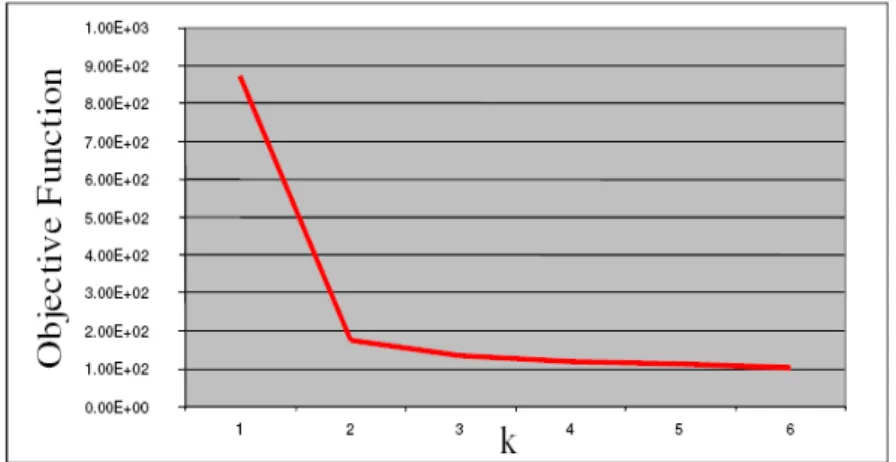
Figure 4. 6 Optimal number of clusters ... 40

Figure 3. 7 The intra distance vs number of cluster ... 40

Figure 3. 8 Influence of the fuzziness parameter m ... 42

Figure 3. 9 Kernel mapping ... 46

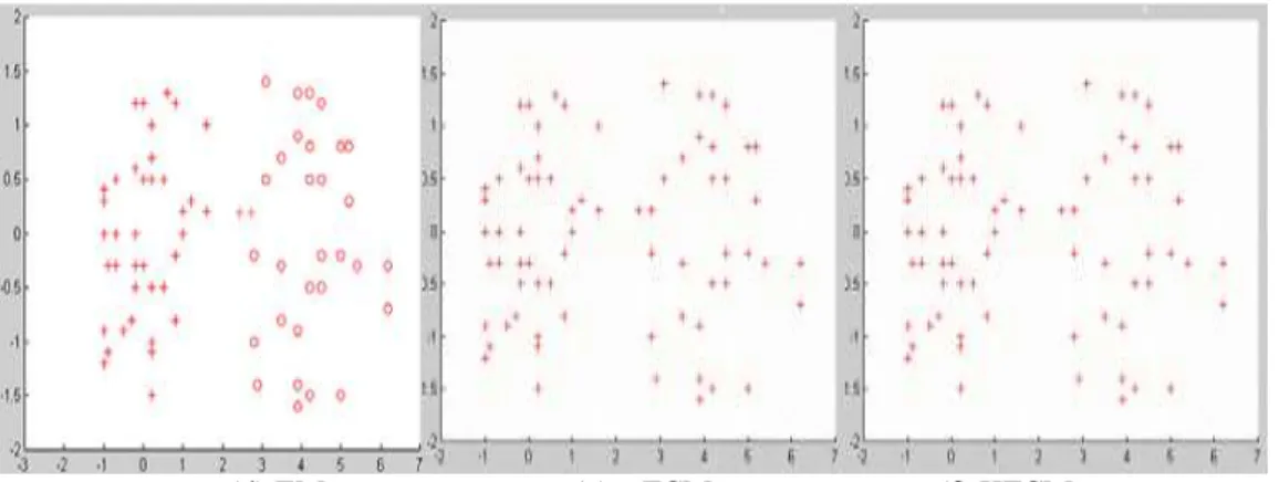
Figure 3.10 Clustering result for two-cluster data ... 51

Figure 3. 11 Clustering result for two-cluster data with noise ... 52

Figure 3. 12 Clustering result for unbalance data ... 52

Figure 3. 13 Clustering result for unbalance data with noise ... 53

Figure 3. 15 ARI for three datasets... 56

Figure 3.16 Relationship between the proposed methods………...……….58

(13)

Figure 4. 2 Clustering result for two-cluster data with noise ... 65

Figure 4. 3 Clustering results for unbalance cluster data ... 65

Figure 4. 5 Clustering result for Ring data ... 66

Figure 4. 6 k neighbours vs adjusted rand index ... 67

Figure 4. 7 Silhouette index for two sets of gene expression data ... 68

Figure 4. 8 ARI for Yeast 384 ... 68

Figure 4. 9 BHI for two sets of gene expression data... 69

Figure 4. 10 FOM for two sets of gene expression data ... 70

Figure 5. 1 ARI vs random initial cluster centre ... 73

Figure 5. 2 Parzen density estimation ... 73

Figure 5. 3 Detection of cluster centres ... 76

Figure 5. 4 Density function with different h ... 78

Figure 5. 5 ARI vs h for Yeast 384 ... 78

Figure 5. 6 Density function with different σ ... 80

Figure 5. 7 ARI vs σ for Yeast 384 ... 80

Figure 5. 8 Ideal distribution in the feature space ... 82

Figure 5. 9 vectors in original space ... 82

Figure 5. 10 Flowchart of DKFCM ... 84

Figure 6. 11 Clustering result for a two cluster data with noise ... 85

Figure 6. 12 Clustering result for unbalance data ... 86

Figure 5. 14 ARI for two gene expression data ... 87

Figure 5. 15 Clustering result by DKFCM for Yeast 384 ... 88

Figure 5. 16 Clustering result by DKFCM for Yeast 237 ... 88

Figure 5. 17 BHI for for two gene expression data ... 89

Figure 5. 18 FOM for two gene expression data ... 93

Figure 5. 19 ARI vs the number of training samples ... 94

Figure 5. 20 ARI vs the number of k minimum distances ... 94

Figure 6. 1 Curve fitting ... 101

Figure 6. 2 Smoothed curves obtained for the gene Cyp4a10 with ... 102

Figure 6. 3 Radius of curvature of a curve ... 103

Figure 6. 4 Radius of curvature with different trend ... 104

Figure 6. 5 ARI for two sets of gene expression data ... 105

(14)

Figure 6. 7 FOM for three sets of gene expression data ... 107

Figure 6. 8 Heatmap of cluster structure for Yeast 384 ... 108

Figure 6. 11 ARI vs Smoothing parameter for Yeast 384 ... 111

(15)

List of Tables

Table 3.1 Fuzzy exponent for datasets ... 43

Table 3. 2 Kernel functions ... 48

Table 3. 3 Sillouette index for optimal number of clusters... 55

Table 3. 4 ARI for optimal number of clusters ... 56

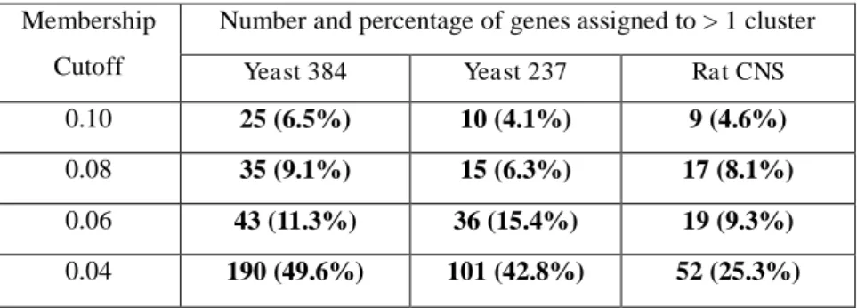
Table 3. 5 Fuzzy assignment of genes to clusters for three gene expression data ... 57

Table 5. 1 vectors vs varying parameter ... 82

Table 5. 2 p-value of Yeast 384 ... 91

(16)

List of Abbreviations

ARI Adjusted Rand Index

BHI Biological Homogeneity Index

BP Biological Process

CC Cellular Component

cDNA Complementary DNA

CLICK Cluster Identification via Connectivity Kernels

DNA Deoxyribonucleic Acid

EM Expectation Maximization

FCM Fuzzy c-mean

FOM Figure of Merit

KFCM Kernel Fuzzy c-means

KNN K-Nearest Neighbours

LFCM Local fuzzy c-means

MF Molecular Function

mRNA Messenger ribonucleic acid

NGMs Neuro-Glial markers

NTRs Neuro-transmitter receptors

PEPS Peptide signaling family

PDF Parzen Density Function

RSS Residual Sum of Squares

SOM Self Organizing Map

(17)

Chapter 1 Introduction

1.1 Overview

Bioinformatics is a new application of computers, mathematical and statistics models to analyses of biological data. There are two important research fields in bioinformatics: genomic analysis and proteomic analysis. Genomic analysis aims to extract information from large amounts of gene data, while proteomic analysis has an objective to determine protein functions from protein databases. The high-throughput technologies can rapidly sequence and analyze the whole genome, which supplies an opportunity to understand the complex cellular interactions. Although the sequencing of genomes has delivered many insights into their com-position, it has offered a static view of genes in various organisms. Questions about the interaction of genes and the impact of environmental conditions on ge-netic networks remain difficult to study using sequence data only (Andreas and Francis, 2005).

Microarray techniques can simultaneously measure the expression of thousands of genes across a collection of related experiments or during biological process, which investigates the dynamic behavior of genes. Interactions in gene networks and responses to environmental changes can be monitored systematically (Andre-as and Francis, 2005). One of the greatest challenges posed by microarray tech-nologies is the analysis of the large amounts of data. Finding meaningful struc-tures and useful information in microarray experiments is a formidable task and demands new approaches of data processing and analysis. These approaches have

(18)

to be exploratory and should not be model dependent, since only a fragment of the underlying data-producing mechanisms is known. Although biological experi-ments provide a wealth of information on genes and proteins, these experiexperi-ments are expensive and time-consuming. Hence computational prediction methods are needed to provide valuable information for large DNA microarray data whose structures or functions cannot be determined from biological experiments.

1.2 Problem definition

The potential applications of microarray data are numerous. Functionally related genes can be detected by clustering of gene based on expression values (Page and Coulibaly, 2008). Medical applications of microarray data analysis seeks to iden-tify genes involved in disease by comparing gene expression values between tis-sues of healthy and diseased individuals (Andreas and Francis, 2005). This is of-ten accomplished by supervised learning techniques for class comparison and class prediction. Moreover, patterns of genes specifically induced in pathological tissues may be identified using clustering techniques (Andreas and Francis, 2005). Finding genes that are common to specific groups of tumors may prove useful. Such findings could offer medical researchers a starting place in their quest to im-prove the reliability of cancer diagnosis and treatment effectiveness. The possibil-ity of gene targeted treatment requires one to more accurately understand the un-derlying genetic and environmental factors which contribute to the development of cancer (Andreas and Francis, 2005). Cluster analysis is one tool in a growing arsenal of research weapons for better understanding these relationships. In recent years, clustering methods have been used extensively in analyzing biological data, especially for DNA microarrays data. Clustering is an important technique by identifying interesting patterns in the data. A key step in the clustering process is the identification of a group of genes that manifest similar expression patterns over several conditions into clusters, thus revealing relations among genes and their functions. A cluster of genes can be defined as a set of biologically relevant genes which are similar based on a proximity measure.

(19)

Developing an effective clustering algorithm frequently involves three steps (Fig-ure 1.1). The first step is to select effective feat(Fig-ures by identifying a subset of the original data. Irrelevant and redundant genes or conditions are excluded for fur-ther analysis. The second step is the clustering process, which utilizes a strategy to find the optimal or sub-optimal groups in the dataset. The strategy is usually based on two components: proximity measure and clustering criterion. A proximity measure quantifies the similarity between two observations, while the clustering criterion is based on the expected distribution of underlying data (such as intra homogeneity and inter separateness). The final step is cluster validation, which

assesses the quality of the clusters. “Good” cluster for gene expression analysis is the one that can be biologically interpreted.

Figure 1. 1 Framework of clustering for gene expression data analysis

Data clustering analysis is a useful tool and has been extensively applied to ex-tract information from gene expression profiles obtained by DNA microarrays. However, existing clustering approaches are mainly developed in computer sci-ence for image processing and pattern recognition, which neglects the specific characteristics of gene expression data or the particular requirements from the bi-ological domain. Therefore, clustering result lacks of reliability and bibi-ological in-terpretation. Moreover, although numerous algorithms have been developed to address the problem of data clustering, these algorithms have their limitations such as determining the number of clusters, selecting the proximity measure.

Data collection Pre-Processing Clustering Validation

(20)

hough some cluster indices address this problem, they still have the drawback of model over-fitting. Alternative approaches, based on statistics with the log-likelihood estimator and a model parameter penalty mechanism, can reduce over-fitting, but are still limited by assumptions regarding models of data distribu-tion and by a slow convergence with model parameter estimadistribu-tion. Even when the number of clusters is known a priori, different clustering algorithms may provide different solutions because of their dependence on the initialization parameters. Because most algorithms use an iterative process to estimate the model parame-ters while searching for optimal solutions, a solution that is a global optimum is not guaranteed.

1.3 Aims and objectives

This thesis aims to investigate the performance of existing clustering techniques and thus to contribute to the development of new clustering techniques for gene expression data. The main objectives are as follows:

1. In order to evaluate the clustering performance for gene expression data, this study reviews a range of clustering techniques and evaluates theirs advantages and disadvantages.

2. Traditional FCM is sensitive to the noise. However, gene expression data involves a large component of noise, which limits its application. The lo-cal structure includes a lot of useful information which can be utilized to accentuate the meaningful data and minimize the noise influence. By pre-serving the local structure, a weighted FCM is proposed.

3. FCM is sensitive to the initialization. In order to solve this sensitivity and avoid FCM trapping into local minimum, an initialization scheme is pro-posed. Moreover, FCM utilizes Euclidean distance to calculate gene simi-larity. It is only effective finding spherical and equal sized clusters, which makes the results lack of biological interpretation. In order to identify general clusters, a density weighted KFCM is proposed.

(21)

4. Time series is a special kind of microarray data. However, conventional clustering methods rarely consider the characteristics of time series. In or-der to find useful information from this type of data, the characteristics of time series is studied and a new clustering approach is proposed which us-es spline to smooth gene exprus-essions. It not only eliminatus-es random varia-ble and noise, but also preserves the general trend of the expression files.

1.4 Thesis contribution

This dissertation focuses on construction of a machine learning and data mining framework for discovery cluster structure with biological significance in gene ex-pression data. Three novel algorithms have been developed:

1. A local weighted FCM method (LFCM) is proposed, which renders LFCM immune to noise by utilizing local structure information. Ex-periments on artificial data and real gene expression data show that the proposed method outperforms the conventional ones.

2. A density weighted KFCM methods (DKFCM) is developed, which incorporates an automatic parameter selection to find the optimal val-ues in the clustering process. This method detects arbitrary shapes of clusters and the clusters are of biological significance in gene expres-sion data analysis.

3. A FCMS method is developed for time series gene expression data, which utilizes spline to smooth gene expression data, and adopts a new proximity measure to compute genes similarity. Experiments show that the proposed method can identify distinct and accurate patterns, which offers biologists an efficient way to understanding the data.

1.5 Thesis structure

(22)

Chapter 1 gives an overview of the thesis. The problem definition, research

ob-jectives and thesis contribution are all addressed.

Chapter 2 discusses the biological foundation of research background, such as

gene theory, microarray technology etc. Literatures on the clustering techniques and validation measures for gene expression analysis are also reviewed.

Chapter 3 describes the dataset used in this research. Data preprocessing, such as

missing values estimation, filtering and standardization are discussed.

Chapter 4 gives an introduction to the FCM and KFCM. KFCM not only finds

the nonlinear relationship between genes, but also detects arbitrary shapes of clusters. A full comparison of FCM and KFCM with other popular algorithms is run using artificial data and real gene expression data.

Chapter 5 reveals the limitations of FCM, which assigns equal weights to genes

without consideration of their contributions to the clustering process. This treat-ment makes the results lack accurate and biological interpretation. A local FCM is proposed by assigning different weights to genes according to their contribution to the clustering. Experiments show that the proposed method achieves better per-formance than the conventional ones.

Chapter 6 proposes a density weighted KFCM approach. An initialization meth-od is presented based on Parzen density estimation. In addition, the objective function is amended by adding a new weighted parameter to accentuate the ob-jects in high density area. Furthermore, a parameter optimization is presented which automatically finds the optimal values in the clustering process. Experi-ments on synthetic data and real gene expression data show that proposed method substantially outperforms conventional models.

(23)

or-der to minimize the noise influence and identify the trend change, cubic spline is used to smooth gene expression. FCM is then used to cluster the splines based on radius of curvature. Experiments results show that the proposed method has better performance than conventional FCM.

Chapter 8 draws a conclusion of the thesis. Some of the major challenges laying

(24)

Chapter 2 Research Background and

Literatures Review

2.1 Microarray and gene expression data

Proteins are the major active elements of cells. They perform many key functions of biological systems and they are the structural building blocks of cells and tis-sues (Andreas and Francis, 2005). The information for producing the proteins re-quired in a cell under a particular condition is contained in the deoxyribonucleic acid (DNA), and the complete DNA sequence of a living organism, the genome, is organized into chromosomes and genes. The production of protein from DNA is divided into two main steps. In step one, known as transcription, single stranded messenger ribonucleic acid (mRNA) is copied from the DNA, and in the second step, known as translation, proteins are produced based on information from the mRNA. This is illustrated as,

DNA  mRNA Protein

Gene expression analysis is the study of mRNA levels transcribed from DNA. In contrast to DNA which is static over the life-time and cells of a living organism, mRNA level varies over time and between cell types. It also varies within cells under different conditions (Andreas and Francis, 2005). For example, the amount of mRNA transcribed from a gene in a healthy organism can differ from the amount of mRNA transcribed from the same gene in the corresponding cell type of a sick organism. Therefore, this gene is differentially expressed between the two conditions healthy and sick.

(25)

Microarray is considered as an important tool for advancing the understanding of the DNA information, molecular mechanisms, and pathophysiology of critical ill-ness. By microarray, the expression of thousands of genes can be assessed and complex pathways can be more fully evaluated in a single experiment. Microar-rays are based on the fundamental principle of base-pair complementarity of nu-cleic acids. Since the binding of different nucleotide strands occurs independently, base-pair complementarity allows parallel probing of complex mixtures of gene transcripts (Andreas and Francis, 2005). There are two major platforms on which microarray experiments are performed: Affymetrix and complementary DNA (cDNA). The primary difference between these designs is that the cDNA proach uses a single long stretch of DNA for each gene while the Affymetrix ap-proach uses several short oligonucleotides to probe for each gene (Andreas and Francis, 2005). The cDNA technology measures the relative gene abundance from two samples while the Affymetrix technology measures the absolute gene abun-dance for a single sample. In the oligonucleotide arrays, each gene is represented by multiple probes of length 20 bp (Andreas and Francis, 2005). These probes are synthesized base by base and are placed in hundreds of thousands of different po-sitions on a glass plate, using photolithography. The arrays are then scanned and the quantitative fluorescence image along with the known position of the probes is used to assess whether a gene is present and its abundance. In the oligonucleotide arrays the fluorescence image is an absolute measure of the abundance of mRNA of a sample. Using solid surfaces to attach cDNAs or oligonucleotides, whole ge-nomes can be studied with a single array. Parallel measurement of gene activities overcomes the limitations of the traditional gene-by-gene approach as whole net-works of interacting genes can be readily studied.

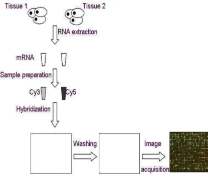
For the cDNA microarray, the DNA from thousands of genes is spotted onto a small glass slide in a regular pattern. Each spot or probe interrogates for a specific gene. Probes are generated by amplifying genomic DNA with gene specific pri-mers. The probes are spotted onto the slide automatically by a robot (Andreas and

(26)

Francis, 2005). mRNA from the samples is purified and reverse transcribed to cDNA with fluorescent labeled nucleotides. If two samples are used (e.g. control and treatment), they are labeled separately with the fluorescent dyes Cyanine-3 (Cy3) and Cyanine-5 (Cy5), which emit light in different spectrums. The spec-trums are assigned the colors green (Cy3) and red (Cy5) for convenience. The la-beled cDNA is mixed in equal amounts and hybridized to the array (Figure 2.1). Unbound cDNA is washed away and the array is scanned twice with a laser, gen-erating one red and one green image (Andreas and Francis, 2005).

Figure 2. 1 Steps in a microarray experiment The Cy3 and Cy5 in the diagram refer to the mRNAs dyed

using the two fluorescent dyes of Cy3 and Cy5.

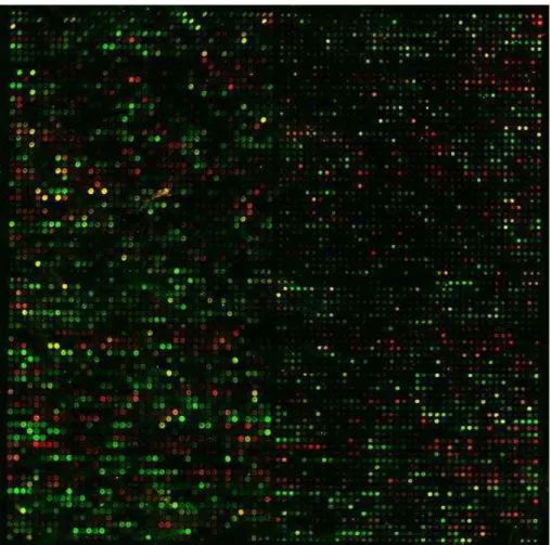
Once the images are overlaid, spots hybridized with equal amounts of control and treatment cDNA are yellow, while spots for genes that ar differentially expressed are different shades of red or green (Andreas and Francis, 2005). The cDNA mi-croarray image is illustrated in Figure 2.2. Various image analysis techniques are employed to identify the red and green intensities in the spots along with the sur-rounding background. Since the spot size and hybridization properties change for different nucleotide sequences, the measured fluorescence intensity cannot be translated to an absolute level of mRNA. The ratio between the amounts of gene specific mRNA in the two samples is called a fold difference, which is often

(27)

in-terpreted as evidence that the gene is differentially expressed.

Figure 2. 2 Scan of a cDNA microarray containing the whole yeast genome (Ben-Dor et al.,1999)

2.2 Clustering Algorithms

Generally, clustering has two main applications for gene expression analysis: gene based clustering and sample based clustering. In gene-based clustering, the genes are treated as the objects, while the samples are the features. While, the samples based clustering regards the samples as the objects and the genes as the features, it partitions samples into homogeneous groups. Each group may correspond to some particular macroscopic phenotype, such as clinical syndromes or cancer types (Golub et al. 1999). The distinction of gene based clustering and sample based clustering is based on different characteristics of clustering tasks for gene expres-sion data. In this research, only gene-based clustering is considered.

(28)

DeRisi et al. (1996) initially revealed expression patterns when they studied the gene expression data of Yeast cell cycle. In order to infer the function of novel genes, they employed clustering analysis by grouping them with genes of well-known functionality. This is based on the observation that genes showing similar expression patterns (co-expressed genes) are often functionally related and are controlled by the same regulatory mechanisms (co-regulated genes). Expres-sion clusters are frequently enriched by genes of certain functions e.g. DNA rep-lication, or protein synthesis. If a gene of unknown function falls into such a clus-ter, it is likely to serve the same functions as other members of the cluster. This method enables assigning possible functions to a large number of genes by clus-tering of co-expressed genes (Chu et al. 1998). Analysis of cluster structure can further identify the underlying mechanisms of metabolic and regulatory networks in the cell. It is especially valuable for organism and cell types where little previ-ous knowledge about their biology exists.

Sample based clustering takes samples as objects and genes as features. It helps to understand gene regulation, metabolic and signaling pathways, the genetic mech-anisms of disease, and the response to drug treatments. For instance, if overpression of certain genes is correlated with a certain cancer, it is promising to ex-plore which other conditions affect the expression of these genes and which other genes have similar expression profiles. It is also valuable to investigate com-pounds (potential drugs) lower the expression level of these genes. Alizadeh et al. (2000) applied a clustering algorithm to large B-cell lymphoma using 96 samples of normal and malignant lymphocytes and found that there is diversity in gene expression among the tumors of diffuse large B-cell lymphoma patients. They identified two molecularly distinct forms of diffuse large B-cell lymphoma, which had gene expression patterns indicative of different stages of B-cell differentia-tion. Interestingly, these two groups correlated well with patient survival rates, thus confirming that the clusters are meaningful. Ayano et al. (2013) employed clustering to differentiate genetic lineages of undifferentiated-type gastric

(29)

carci-nomas analysed of genomic DNA microarray data. The goal of sample based clustering is to find the phenotype structures or substructures of the sample. Alt-hough the conventional clustering methods, such as k-means, SOM, hierarchical clustering can be directly applied to cluster samples using all the genes as fea-tures, the irrelevant genes may seriously degrade the quality and reliability of clustering results (Xing and Karp, 2001). Thus, particular methods should be ap-plied to identify informative genes and reduce gene dimensionality for clustering samples to detect their phenotypes. In this study, sample based clustering is out of the research scope.

Recently, many methods for cluster analysis have been proposed, such as k-means, hierarchical clustering, self-organizing maps, and graph theoretic approaches. These algorithms are also applied to analysis of microarrays.

(1) k-means

The k-means is the most widely used clustering method, which partitions n ob-jects into k clusters, and each objects belongs to its nearest cluster centres (Steinley, 2006). The objective function is,

2 1 1 ( , ) C N ij j i i j J d x v   



(2.1)

where C and N denote the number of clusters and objects respectively, x_jin the j th objects. 2₍ _{, )}

ij j i

d x v is the distance between vector x_j and prototype v_i.

dij2( , )x vj i arg min



dij2( , )x vj i



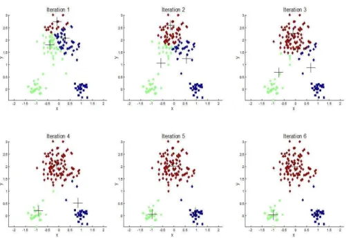
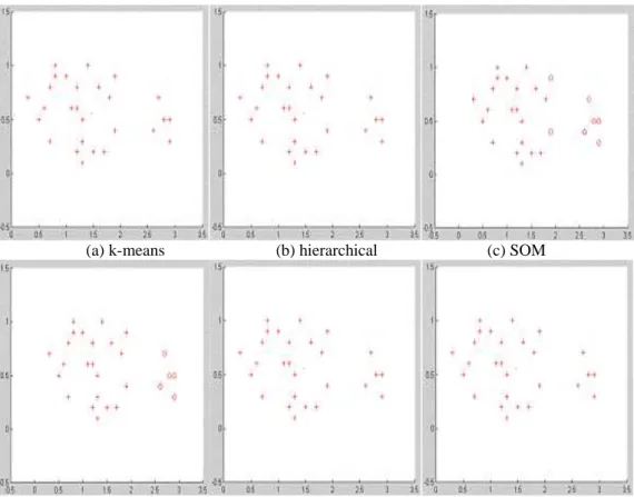
(2.2) The k-means aims at minimizing the intra-cluster distance, which starts with se-lection of k cluster centres. Then, each object in the dataset is assigned to the closest cluster. After that, the cluster centres are recalculated according to the as-sociated objects. This process is repeated until convergence is achieved. Figure 2.3 is an illustration of the process of k-means, in the first iteration; three initial cluster centres are randomly selected with symbols “+”, and it converges to the

(30)

minimum in the sixth iteration.

Figure 2. 3 The illustration of the k-means process with six iterations steps

The k-means algorithm is easy to implement and its time complexity is suitable for large datasets. However, k-means need user to specify the number of clusters which is usually unknown in advance. In order to detect the optimal number of clusters, users usually run the algorithms repeatedly with different values of k and compare the clustering results. For large gene expression dataset which contains thousands of genes, this extensive parameter fine-tuning process may not be prac-tical. Moreover, k-means forces each gene into a cluster, this compulsive strategy may cause the algorithm to be sensitive to noise (Steinley, 2006). Finally, k-means leads to local minimum of the objective function, thus the clustering re-sult depends on the initiation. To reduce the influence of the initial partition on the clustering result, one can run the algorithm multiple times then choose the result that has the minimal cost function.

Recently, many advanced clustering algorithms based on k-means have been pro-posed to overcome the drawbacks. Steinley (2003) gave a deep discussion on the k-means local optima and proposed a solution to avoid the algorithm trapping in local optima. However, the qualities of clusters in gene expression datasets vary widely. Thus, it is difficult to choose the appropriate globally-constraining

(31)

param-eters. Similarly, Tseng (2007) proposed a penalized and weighted k-means for clustering with scattered objects, which have been applied in gene expression data, and can find tightly meaning clusters. Genetic algorithm was combined with k-means for clustering large-scale microarray data (Wu, 2008). Compared with the original approach, the new method is able to capture clusters with complex and high-dimensional structures accurately. Iam-On and Boongoen (2012) pre-sented a new weighted k-means for microarray data by learning the local structure, which can effectively identify the cancer relating genes and aid the biologists to find the subcategories of cancer.

(2) Hierarchical clustering

There are two basic types of hierarchical clustering methods: agglomerative and divisive clustering. The agglomerative method starts with taking each object as a cluster and merges objects into groups according to their similarities. In the first iteration, the most similar objects are grouped together and merged. In the final iteration, all of the objects are contained in a single large cluster. In each iteration, the method fuses the objects which are the most similar. Figure 2.4 shows the ag-glomerative clustering process and the tree structure. According to the similarities between clusters, agglomerative method can be divided into: single linkage, com-plete linkage and average linkage. The single linkage method considers the short-est pairwise distance between objects in two different clusters as the distance be-tween the two clusters (Guess and Wilson, 2002). While the complete linkage method defined the distance as the most distant pair of objects (Guess and Wilson, 2002). As the average linkage clustering, the average of the pairwise distances between all pairs of objects coming from each of the two clusters is taken as the distance between two clusters (Guess and Wilson, 2002). On the contrary, divisive method starts with all of the objects contained in one large cluster. In each itera-tion, the groups are subdivided or kept in the same cluster based on how close the individuals within clusters are in terms of their similarity measures. Eventually, there are as many clusters as individuals (Guess and Wilson, 2002).

(32)

.

Figure 2. 4 An illustration of Hierarchical clustering process

Compared with k-means, hierarchical approach is not sensitive to initialization and is robust to the noise (Guess and Wilson, 2002). In addition, the number of clusters needs not to be specified a priori and it can graphically represent the da-taset, which provides the user a thorough impression of the data distribution. However, the clustering procedure is static, patterns assigned to a cluster cannot move to another cluster. It fails to separate overlapping clusters due to a lack of information about the global shape or size of the clusters (Boratyn et al., 2006).

Lewis, and Noble (2003) describe a generalization of the hierarchical clustering algorithm that efficiently incorporates high-order features by using a kernel func-tion to map the data into a high dimensional feature space. Makretsov et al. (2004) used a hierarchical clustering in tissue microarray immunostaining data and suc-cessfully identifies prognostically significant groups of breast cancer. Inamura et al. (2005) combines non-negative matrix factorization and hierarchical clustering to find two subclasses of lung squamous cell carcinoma with different gene ex-pression profiles and prognosis. Boratyn et al. (2006) used certain biological knowledge to supervise the hierarchical clustering, and produced clusters with more biological significance, which outperformed the conventional hierarchical clustering algorithms substantially. Trevino et al. (2012) presented a hierarchical clustering for Escherichia coli data and identify distinct gene expression patterns. Badsha et al. (2013) proposed a robust hierarchical clustering method with respect

(33)

to the noise by maximizing the β-likelihood function for a gene expression data.

(3) Self-organizing map

Self-organizing map (SOM) is a type of artificial neural network that is trained using unsupervised learning to produce a low-dimensional, discretized representa-tion of the input space (Kohonen, 1984). Initially SOM constructs geometry of nodes (a 7 x 9 grid in Figure 2.5). Each node is associated with a reference vector, and the input vectors are mapped to the node with the closest reference vector. The location of the nodes is iteratively adjusted by moving in the direction to the dense areas of the input vector space (Torkkola et al., 2001). Once the algorithm has proceeded through a user defined number of iterations, it terminates with sim-ilar objects grouped around a specific node.

Figure 2. 5 Self-organizing map (Kohonen, 1984)

Torkkola et al. (2001) applied SOM to exploratory analysis of microarray data and found SOM not only enabled quick selection of the gene families identified in previous work, but also facilitated the identification of additional genes with sim-ilar expression patterns. Covell et al.(2003) used SOM analysis of microarray data for molecular classification of cancer. Similarly, Hautaniemi et al. (2003) applied SOM to analysis and visualization of gene expression microarray data of human cancer and found a set of potential predictor genes for classification purposes. Comparison and visualization of the effects of different drugs is straightforward with SOM (Dragomir et al., 2004). Dragomir et al (2004) used SOM to explore

(34)

the microarray data by incorporating independent component analysis (ICA) to reduce data features. Wu et al. (2005) proposed a hybrid SOM-SVM approach for the zebrafish gene expression analysis by utilizing a small portion labeled genes to train the model, and then clustering pattern, results showed that this method is ca-pable of finding certain biologically meaningful clusters.

(4) Graph-theoretical algorithm

Given a dataset X, a proximity matrix P can be constructed where

( , ) ( , )

P x y  proximity x y and a weighted graph G V E( , ), where each data cor-responds to a vertex. For clustering methods, each pair of objects is connected by an edge with weight assigned according to the proximity value between the ob-jects. Graph-theoretical clustering techniques are explicitly presented in terms of a graph, thus converting the problem of clustering a dataset into such graph theoret-ical problems as finding minimum cut or maximal cliques in the proximity graph

G. Cluster Identification via Connectivity Kernels (CLICK) is a representive graph-theoretical algorithm which has been successfully used for gene expression analysis and produced high quality clusters (Roded et al., 2003). CLICK seeks to identify highly connected components in the proximity graph as clusters. CLICK makes the probabilistic assumption that after standardization, pairwise similarity values between elements are normally distributed. Under this assumption, the weight_ijof an edge is defined as the probability that vertices i and j are in the same cluster. The clustering process of CLICK iteratively finds the minimum cut in the proximity graph and recursively splits the data set into a set of connected components from the minimum cut. CLICK also takes two post-pruning steps to refine the cluster results. The adoption step handles the remaining singletons and updates the current clusters, while the merging step iteratively merges two clusters with similarity exceeding a predefined threshold (Roded et al., 2003). Clusters obtained by CLICK demonstrated better quality in terms of homogeneity and sep-aration. However, CLICK has little guarantee of not going astray and generating highly unbalanced partitions, e.g., a partition that only separates a few noises from the remaining data objects (Roded et al., 2003). Furthermore, in gene expression

(35)

data, two clusters of co-expressed genes may be highly intersected with each other. In such situations, CLICK is unable to identify the two clusters and reported as one highly connected component (Roded et al., 2003).

(5) Model-based clustering

The mixture models approach assumes that the data are from a mixture of a speci-fied number of groups in various proportions. By assuming a parametric form for the density function in each group, a likelihood function can be formed in terms of a mixture density (Dempster et al., 1977). The unknown parameters of the distri-bution can be estimated by the method of maximum likelihood. This process leads to estimates of cluster specific parameters as well as the proportion of observa-tions falling in each cluster and the posterior probability of each observation fall-ing in a specific cluster. Clusterfall-ing proceeds by assignfall-ing each object to a group based on the relative value of the estimated posterior probability of belonging to that group compared with the posterior probabilities of belonging to the other groups.

The Expectation/Maximization (EM) algorithm is a two-stage iterative algorithm, which consists of expectation and maximization steps (Dempster et al., 1977). The expectation step estimates the data by calculating expected values conditional on the observed data. Once the data are estimated in the expectation step, the maximum likelihood estimates of the parameters are calculated in the maximiza-tion step. The EM algorithm requires starting values for the parameter estimates to be input for the first expectation step (Dempster et al., 1977). One of the ad-vantages of the mixture models for analyzing microarray data is that they provide a statistical criterion for assessing the number of clusters present in the data. A strong assumption made in fitting mixture models to microarray data is that the genes are independent and identically distributed according to the mixture density. However, the EM algorithm converges slowly, particularly at regions where clus-ters overlap and requires the data distribution to follow some specific distribution model (Yeung et al. 2001a). Moreover, gene expression data is likely contain

(36)

overlapping clusters and do not always follow standard distributions, (e.g., Gaussian), which is inappropriate for such kind of data.

Given various clustering methods, however, there is no one clustering algorithm that performs significantly better than the others when tested across multiple da-tasets. This is due to microarray data tends to have complex biological system and diverse structures (Andreas and Francis, 2005).

2.3 Validation measures

Different methods frequently yield different clustering results. Thus, a fair com-parison between alternative clustering methods is necessary. However, there is no benchmark for the critical assessment of any clustering approach in the field of gene expression data analysis. In order to ensure the quality of the clustering algo-rithm and compare the clustering performance, many validation methods have been proposed based on statistical models for comparison of clustering approach-es with a controlled number of clusters. Generally, they can be classified into three categories: internal measure, external measure, and biological measure.

2.3.1 Internal measure

Internal measures assess the quality of the clustering approaches using intrinsic information of the dataset. Silhouette index and Figure of merit are selected as the internal validation in this work.

Silhouette index

Silhouette index is a measure of tightness and separation of clusters, which is used to assess the level of statistical significance of clusters. For a given cluster X_j ( j1,....,c), this method assigns each sample X_j a quality measure, s i( ) (i1,....,m), known as the Silhouette width. The Silhouette width is a confidence

(37)

indicator on the membership of the i th sample in clusterX_j. The Silhouette width for the i th sample in cluster X_j is defined as,





( ) ( ) ( ) max ( ), ( ) b i a i s i a i b i   (2.3)

where a i( ) is the average distance between the i th object and all of the objects included in X_j, and b i( )is the minimum average distance between the i th sample and all of the samples clustered in X (_k k1,...., ;c k j), and this formula follows that  1 s i( ) 1 . s(i) closing to 1 indicates that the i th object has been well clustered, i.e. it was assigned to an appropriate cluster. s(i) closing to zero suggests that the i th sample could be assigned to the neighboring cluster. If s(i) is close to –1, one may argue that a object has been misclassified. Thus, for a given cluster, X_j( j1,....,c), it is possible to calculate a cluster SilhouetteS_j, which characterizes the heterogeneity and isolation properties of such a cluster,

1 1 ( ) m j i S s i m _ 



(2.4)

where m is the number of samples in S_j. It has been shown that for any partition 1

: .... _i .... _c

U X  X  X , a Global Silhouette value,GS , _u can be used as an effective validity index, 1 1 c u j j GS S c _ 



(2.5)

The partition with the higher GSu is taken as the optimal partition. It is should be note that the internal validation has a limitation that clusters are validated using the intrinsic information from the data.

Figure of merit

Figure of merit (FOM) reveals the reliability of the resulting clusters, which indi-cates the probability of the clusters is not formed by chance. It is based on the

(38)

concept that if a clustering result reflects true cluster structure, then a predictor based on the resulting clusters should accurately estimate the cluster labels for new test samples. For gene expression data, extra data objects are rarely used as test samples, since the number of available samples is limited. Rather, a cross-validation method is applied. The generated clusters are assessed by repeat-edly measuring the prediction strength with one or a few of the data objects left out in turn as “test samples” while the remaining data objects are used for cluste r-ing. Intuitively, genes within the same clusters are expected to have similar ex-pression levels, while genes in disjoint clusters are expected to be relatively far apart from each other. Therefore, FOM is the ratio of the within-cluster dispersion to the between-cluster separation. The FOM is defined as follows,

1 m a x m i n 1 ( , ) ( ( , ) 1 ( ( ) ( ) 1 i i i k i i x C C C R x e C e n FOM e k e e k         



(2.6)

where n is the number of genes, k is the number of clusters, R x e( , ) is the ex-pression level of gene x under condition e and C ei( ) is the average expression level in condition e of genes in cluster C_i. The FOM measures the mean devia-tion of the expression levels of genes in e relative to their corresponding cluster means. Thus, a small value of FOM indicates strong prediction strength, and therefore a high level reliability of the resulting clusters.

2.3.2 External validation

External validation assesses the degree of consensus between the clustering result and the class labels. Rand index (RI) is a measure of agreement between two par-titions: one is the clustering result and the other is the standard partition (Given by external information). The RI computes the proportion of the total observation pairs that agree (Everitt et al., 2001). Agreement means that either both of the ob-servations in the pair fall into the same cluster according to both partitions or both observations fall into different clusters according to both partitions. Suppose T is

(39)

the true clustering of a gene expression data based on biological knowledge and C is a clustering result given by certain clustering algorithm. Let a denote the num-ber of gene pairs belonging to the same cluster in both T and C, b is the number of pairs belonging to the same cluster in T but to different clusters in C, c is the number of pairs belonging to different clusters in T but to the same cluster in C and d is the number of pairs belonging to different clusters in both T and C. The Rand index (RI) is computed by,

( , ) a d RI T C a b c d      (2.7)

The RI has an expected value slightly greater than 0. If the partitions agree per-fectly, the RI is 1. The value of RI varies from 0 to 1 and higher value indicates that the clustering result is more similar to the standard partitions. However, a major problem with the RI is that the expected value of two random partitions does not take a constant value.

Adjusted Rand index (ARI) is proposed by Hubert and Arabie (1985) and it is more sensitive than the RI. ARI assumes the generalized hyper geometric distri-bution as the model of randomness. The general form of ARI is,

2 ( - ) ( + ) ( + ) + ( + ) ( ( , ) ) ad bc a b b A d a c c R T C d I  (2.8)

ARI has an expected value of zero and ranges from -1 to 1. where negative values indicate poor clusters, while positive values means significant clustering methods. When ARI attains 1.0, the clustering method is the perfect. The RI and ARI are frequently used to assess the quality of clusters for microarray data (Yeung et al., 2001; Yeung and Ruzzo, 2001).

The following example illustrates the computation of RI and ARI. Given a dataset including 5 items and 2 clustering partitions:

Clustering A: 1, 2, 2, 1, 1 Clustering B: 2, 1, 2, 1, 1

(40)

In order to calculate the parameters a, b, c, and d, all possible pairs are listed cor-responding to the elements of the two clustering. In total, there are 2

5 10

C 

possi-ble pairs:[1; 2]; [1; 3]; [1; 4]; [1; 5]; [2; 3]; [2; 4]; [2; 5]; [3; 4]; [3; 5]; [4; 5]. For example, the term of [2; 3] is correspond to the pair (2; 2) in clustering A and (1; 2) in clustering B. The parameters are computed by,

CA, [1,2] -> (1,2) -> 1 2 d = + 1 CB, [1,2] -> (2,1) -> 2 1  _     CA, [1,3] -> (1,2) -> 1 2 b = + 1 CB, [1,3] -> (2,2) -> 2 = 2  _    CA, [1,4] -> (1,1) -> 1 = 1 c = + 1 CB, [1,4] -> (2,1) -> 2 1  _    C A , [ 1 , 5 ] - > ( 1 , 1 ) - > 1 = c = + C B , [ 1 , 5 ] - > ( 2 , 1 ) - > 2  _    CA, [2,3] -> (2,2) -> 2 = 2 c = + 1 CB, [2,3] -> (1,2) -> 1 2  _    CA, [2,4] -> (2,1) -> 2 1 b = + 1 CB, [2,4] -> (1,1) -> 1 = 1  _    CA, [2,5] -> (2,1) -> 2 1 b = + 1 CB, [2,5] -> (1,1) -> 1 = 1  _    CA, [3,4] -> (2,1) -> 2 1 d = + 1 CB, [3,4] -> (2,1) -> 2 1  _     C A , [ 3 , 5 ] - > ( 2 , 1 ) - > 2 d = + C B , [ 3 , 5 ] - > ( 2 , 1 ) - > 2  _     CA, [4,5] -> (1,1) -> 1 = 1 a = + 1 CB, [4,5] -> (1,1) -> 1 = 1  _  

According to equation (2.7) and (2.8), RI and ARI can be computed by,

a+b 1+3 a+b+c+d 1+3+3+3 0.4 RI    (2.9) 2 ( 1 2 ( - ) ( + ) ( + ) + ( + ) ( + ) 3 3 3 ) 0 . 2 5 ( 1 3 ) ( 3 3 ) ( 1 3 )3 ( 3 ) a d b c a b b d a c A I c R d                (2.10)

2.3.3 Biological validation

Biological validation evaluates the ability of a clustering algorithm to produce bi-ologically meaningful clusters. Biological homogeneity index (BHI) measures how homogeneous the clusters are biologically (Datta and Datta, 2006). Consider

1 2 3

{ , , ... _F}

B B B B B be a set of F functional classes, not necessarily disjoint, and B(i) be the functional class containing gene i (with possibly more than one functional class containing i). Similarly, B(j) is the function class containing gene

(41)

j, if B(i) and B(j) match (any one match is sufficient in the case of membership to multiple functional classes), it indicates that the two genes have similar biological function by assigning an indicator I B i( ( )B j( ))=1 if else, I B i( ( )B j( ))=0. Intuitively, it is expected that genes placed in the same statistical cluster also be-long to the same functional classes. Then, for a given clustering partition

1 2 3

={C ,C , C ...C }_K

C and set of biological classes B, the BHI is defined as,

1 1 1 ( , ) ( ( ) ( )) ( 1) k K k k k i j C BHI C B I B i B j K _ n n _{ }   



(2.11)

where n_k n C( _kB) is the number of annotated genes in statistical clusterC_k. The BHI is in the range [0, 1], with larger values corresponding to more biological homogeneous clusters.

2.4 Pre-processing for Microarray Data

2.4.1 Data preparation

The aim of microarray experiments is to investigate the activity patterns of genes. However, microarrays do not assess gene activities directly, but by measuring the fluorescence intensities of labeled target cDNA hybridized to probes on the array. Generally, the first step in the analysis of microarray data is the transformation of the fluorescence signals into quantities for gene expression analysis. Although the ratio (intensities of two signals ratio) provides an intuitive measure of expression changes, it has the disadvantage of treating up and down regulated genes differ-ently. For example, genes up regulated by a factor of 2 have an expression ratio of 2, while those down regulated by the same factor have an expression ratio of (– 0.5). The most widely used transformation of the ratio is the logarithm base 2, which has the advantage of producing a continuous spectrum of values and treat-ing up and down regulated genes in a similar fashion. Recall that logarithms treat numbers and their reciprocals symmetrically: log2(1) = 0, log2(2) = 1, log2(1⁄2) =

(42)

are also treated symmetrically, so that a gene up regulated by a factor of 2 has a log2(ratio) of 1, a gene down regulated by a factor of 2 has a log2(ratio) of −1, and

a gene expressed at a constant level (with a ratio of 1) has a log2(ratio) equal to

zero. For the remainder of the dissertation, log2(ratio) will be used to represent

expression levels.

Gene expression data from a microarray experiment can be represented by a re-al-valued expression matrix (Figure 2.6), where the rows represent expression patterns of genes, the column represent the expression profiles of samples, and

each cell is the measured expression level of a gene in certain sample.

Figure 2. 6 Gene expression matrix

2.4.2 Missing values

In gene expression analysis, complete information is preferred throughout the ex-periment. Unfortunately, real datasets frequently have missing values, which is caused by errors or by random noise. For example, sensor failures in a control system may cause the system to miss information. The missing values can also come from the platform level, such as insufficient resolution, image corruption, spotting, scratches or dust on the slide, or hybridization failure. According to Cho et al. (1998), Yeast cell cycle data contained over 6000 missing measurement val-ues that accounts for 6% of the total expression valval-ues. However, most clustering algorithms do not allow for missing values. In order to adapt to the clustering al-gorithms, two approaches have been widely used to address the problem of

(43)

miss-ing values. The simple one is to ignore the genes includmiss-ing missmiss-ing values. This measure is adopted when the proportion of incomplete data is small, but the elim-ination brings a loss of information. The other one is the imputation-based ap-proach, which supplies missing values by certain means of approximation. K nearest neighbors (knn) is a popular method to compute the missing values. A missing value of gene i at time point t is estimated by the average values for time t of the several nearest neighboring genes j. The distance was calculated by,

2 2 ( _i, _j) ( _ik _jk) k n d g g g g n m  _



 (2.12)

whereg_iis the gene expression vector for gene i, g_jis the gene expression vector for neighboring gene j, n is the number of arrays in the time-course experiment and m is the number of measurements which are missing for gene i or j or both. The sum includes only measurements for which both gene expression values (g_ik,g_jk)are present. This procedure exploits the high correlation between genes in expression data. It assumes that genes which are well correlated for existing measurements are also correlated for missing measurements. According to Troyanskaya et al., (2001), knn is an effective measure to estimate the missing values in gene expression data.

2.4.3 Filtering

In one biological process, not all genes show obvious variation according to dif-ferent experiment conditions. Genes expressed at low levels or show small changes are useless for clustering. Involving these data in clustering process will not only increase the redundancy of the data, but also decrease the quality of the result. In order to identify the potential pattern effectively, most clustering ap-proaches include a filtering step to remove these genes.

The commonly used method for gene filtering is based on the variability of gene expression values for a given gene. Genes whose expression values do not change

(44)

by more than a specified value across the samples are filtered out. The logic be-hind this type of filtering is that gene expression values for a gene active in a spe-cific biological process should change at some point. Filtering based solely on variability works well in some cases.

However, no consideration is given to the baseline levels of gene expression. Genes that are naturally lowly expressed will have small variances. These genes could be incorrectly removed if a small change in expression values is biological-ly significant. Specifying a single variance threshold for determining whether or not to keep a gene implies the assumption that all of the genes have similarly scaled variances. This may not always be true. For example, a gene with a large mean and variance for its expression level is of less interest than a gene with a small mean and the same large variance. One might consider using a filtering technique based on the coefficient of variation in this situation. The coefficient of variation gives a measure of the variability in relation to the magnitude of the es-timate and is calculated by dividing the eses-timate by its standard error.

2.4.4 Standardization

For cluster analysis, co-expressed genes frequently show similar changes in ex-pression but may differ in the overall exex-pression rate. Therefore, gene exex-pression vectors have to be standardized. Since most clustering algorithms performed in Euclidian space, co-expressed genes may thus be wrongly assigned to different clusters. Therefore, it is necessary to standardize the expression values of genes by a mean of zero and a standard deviation of one to ensure that vectors of genes with similar changes in expression are close. In standardization, the mean over all the experiments of a gene is subtracted from the expression level of the gene, and the difference is then divided by the standard deviation of the expression levels of the gene over all the experiments. Although normalization is only an intermediate step in the analysis, it has a considerable influence on the final results. The nor-malization equation as follows (Hoffmann et al., 2002),

(45)

2 ( ) i i i i i g g g g g   



(2.13)

For example, three hypothetical genes A, B and C are given, and their expression levels have been measured in normal tissue samples and diseased tissue samples. The results of these measurements are displayed in Figure 2.7 (a). Genes A and B are tightly co-regulated and differentially expressed across tissue types but they are expressed at different level. Gene C is not differentially expressed across tis-sue types but happens to have average expression levels similar to that of gene A. It is expected to find clusters that place genes A and B together but would not cluster them with gene C which is constant across all tissue samples. If clustering using the raw expression profiles, genes A and B will be separated. Figure 2.7 (b) shows the expression profiles for the same three genes after normalization across samples. In this transformed data, the expression values for genes A and B are closely aligned. In contrast, the values for gene C fluctuate randomly. This trans-formation results in that genes A and B being clustered in one group.

(a) Untransformed expression (b) Normalization Figure 2. 7 Untransformed expression vs Normalization

2.5 Datasets

(46)

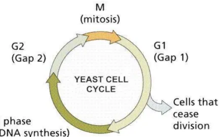
ap-proximately 6000 genes over two cell cycles (17 time points). Tavazoie et al. (1999) selected 384 genes expression profiles, which peak at different time points corresponding to the five phases (G1, S, G2/M, M/G1 and S/G2) of cell cycle. The cell division contains four main phases G1, S, G2, and M shown in Figure 2.8. The division process begins at G1 phase where the cell is prepared for duplication. DNA is replicated in the phase S. In G2 phase, the cell is prepared for cell division. The final phase M is for mitosis, in which a cell is divided into two daughter cells. G2/M, M/G1 and S/G2 are the transition phase.

Figure 2. 8 Yeast cell cycle process

(2) Yeast 2945: Tavazoie et al., (1999) selects 2945 genes by excluding values at time points 90 and 100 minutes. These data sets have already been normalized, where the average expression values are zero and the standard deviation is one.

(3) Yeast 237: Tavazoie et al., (1999) extract 237 genes from the full Yeast cell cycle data which correspond to four functional classes: DNA synthesis and repli-cation, organization of centrosome, nitrogen and sulphur metabolism, and ribo-somal proteins. The resulting 237x17 data matrix is standardized.

(4) Rat CNS: This dataset consists of 112 genes in 9 time points. Wen et al. (1998) suggested that four major gene families are in this data: Neuro-Glial markers fam-ily (NGMs), Neuro-transmitter receptors famfam-ily (NTRs), Peptide signaling famfam-ily

(47)

(PepS) and Diverse (Div).

(5) Serum: This dataset contains 517 genes with 12 expression values (Iyer et al., 1999). The expression of these genes varies in response to Serum concentration in human fibroblasts. Although there is no external criterion for this data set, Iyer et al (1999) suggests five various biological groups in this data.

The dataset’s name, source and size are listed in Table 2.1. Optimal number of clusters in datasets are also specified.

Table 2. 1 Parameters of Gene expression data

Data name Source Size Optimal

num-ber clusters

Yeast 384 Cho et al.(1999)

http://faculty.washington.edu/kayee/data.html

384 x 17 5

Yeast 2945 Tavazoie et al.(1999)

https://tavazoielab.c2b2.columbia.edu/lab/

2945 x 17 16

Yeast 237 Tavazoie et al.(1999)

237 x 17 4

Rat CNS Wen et al. (1998)

112 x 9 4

Serum Iyer et al. (1999)

Http://www.sciencemag.org/feature/data

(48)

Chapter 3 Fuzzy c-means and kernel

fuzzy c-means for gene expression

analysis

3.1 Introduction

This chapter introduces the fuzzy c-means algorithm (FCM), by which a data item may belong to more than one cluster with different degrees of membership. Then a discussion of the parameter selection is presented. FCM is not robust to the noise and only effective finding spherical clusters, both of them limit its applica-tion for gene expression data analysis. Kernel fuzzy c-means (KFCM) is then presented which maps data onto a high dimensional feature space in order to in-crease the representation capability of linear machines. Experiments on artificial data and real gene expression showed that KFCM are more efficient and reliable.

3.2 Fuzzy theory

The mathematical models reviewed in Chapter 2 are crisp, deterministic, and pre-cise in character, which means dichotomous, yes-or-no rather than more-or-less. However, the problems in the