Numerical Methods for the Solution of Partial Differential Equations

(1)

Numerical Methods for the Solution of Partial

Differential Equations

Lecture Notes for the COMPSTAR School on Computational

Astrophysics, 8-13/02/10, Caen, France

Luciano Rezzolla

Albert Einstein Institute, Max-Planck-Institute for Gravitational Physics,

Potsdam, Germany

Available also online at

www.aei.mpg.de/

∼

rezzolla

(2)

Acknowledgments

I am indebted to the several students who have helped me with the typing of the lectures notes into at TEXformat. They are too numerous to be reported here but my special thanks go to Olindo Zanotti for his help with the hyperbolic equations and to Gregor Leiler for his help with the parabolic equations and Chapter 4.

(4)

(5)

Chapter 1

Introduction

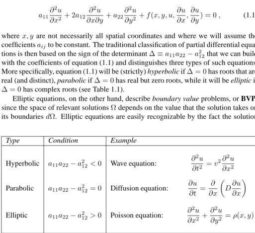
Let us consider a quasi-linear partial differential equation (PDE) of second-order, which we can write generically as

a11∂ 2_u ∂x2 + 2a12 ∂2_u ∂x∂y +a22 ∂2_u ∂y2 +f(x, y, u, ∂u ∂x, ∂u ∂y) = 0, (1.1)

wherex, y are not necessarily all spatial coordinates and where we will assume the coefficientsaijto be constant. The traditional classification of partial differential

equa-tions is then based on the sign of the determinant∆≡a11a22−a212that we can build

with the coefficients of equation (1.1) and distinguishes three types of such equations. More specifically, equation (1.1) will be (strictly) hyperbolic if∆ = 0has roots that are real (and distinct), parabolic if∆ = 0has real but zero roots, while it will be elliptic if

∆ = 0has complex roots (see Table 1.1).

Elliptic equations, on the other hand, describe boundary value problems, or BVP, since the space of relevant solutionsΩdepends on the value that the solution takes on its boundariesdΩ. Elliptic equations are easily recognizable by the fact the solution

Type Condition Example

Hyperbolic a11a22−a212<0 Wave equation:

∂2_u

∂t2 =v 2∂2u

∂x2

Parabolic a11a22−a212= 0 Diffusion equation:

∂u ∂t = ∂ ∂x D∂u ∂x

Elliptic a11a22−a212>0 Poisson equation:

∂2_u

∂x2 +

∂2_u

∂y2 =ρ(x, y)

Table 1.1:Schematic classification of a quasi-linear partial differential equation of second-order. For each class, a prototype equation is presented.

(6)

does not depend on time coordinatetand a prototype elliptic equation is in fact given byPoisson equation(cf. Table 1.1).

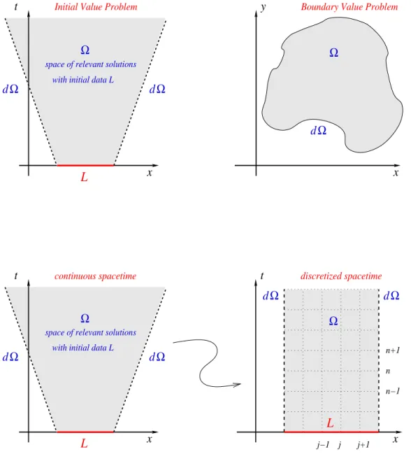
Hyperbolic and parabolic equations describe initial value boundary problems, or

IVBP, since the space of relevant solutionsΩdepends on the value that the solutionL

(which we assume with compact support) takes on some initial time (see upper panel of Fig. 1.1). In practice, IVBP problems are easily recognizable by the fact that the solution will depend on the time coordinatet. Very simple and useful examples of hyperbolic and parabolic equations are given by thewave equationand by the diffu-sion equation, respectively (cf. Table 1.1). An important and physically-based differ-ence between hyperbolic and parabolic equations becomes apparent by considering the “characteristic velocities” associated to them. These represent the velocities at which perturbations are propagated and have finite speeds in the case of hyperbolic equations, while these speeds are infinite in the case of parabolic equations. In this way it is not difficult to appreciate that while both hyperbolic and parabolic equations describe time-dependent equations, the domain of dependence in a finite time for the two classes of equations can either be finite (as in the case of hyperbolic equations), or infinite (as in the case of parabolic equations).

1.1

Discretization of differential operators and variables

Consider, for simplicity, a generic one-dimensional IVBP that could be written as

L(u)−f = 0, (1.2)

whereu=u(x, t)and_Lis a differential operator in the two variablesxandtacting onu. One of the most used methods for the solution of such a problem is by means of

finite differences. It consists in two “discretization steps”:

• Variables discretization: replace the functionu(x, t)with a discrete set of values {un

j}that should approximate the pointwise values ofu, i.e.,unj ≈u(xj, tn);

• Operator discretization: replace the continuous differential operator _L with a discretized one,_L∆, that when applied to the set{u

n

j}, gives an approximation

to_L(u)in terms of differences between the variousun j.

The set of valuesu˜ ≡ {un

j, j = 1, . . . , J, n = 1, . . . , N}(J andN are the number

of points considered for the space and time variable respectively) is called the grid

function and will be denoted by˜u. After this discretization process, the problem (1.2) is replaced by

L∆(˜u)−f˜= 0 +ǫT , (1.3) that is, a discrete representation of both the differential operator_Land of the variable

u. The above equation is the discrete representation of the problem (1.2). Note that the righ-hand-side of (1.3) is not exactly zero and it differs from it by the truncation error

ǫT, which will be introduced in Sect. 1.2.3

In the following Sections 2–7 we will concentrate on partial differential equations of hyperbolic type. Before doing that, however, it is useful to discretize the continuum

(7)

1.2. ERRORS 5 space of solutions (a “spacetime” in the case of IVBPs) in spatial foliations such that the time coordinatetis constant on each slice. As shown in the lower panel of Fig. 1.1, each point_P(xj, tn)in this discretized spacetime will have spatial and time coordinate

defined as

xj =x0+j∆x , j= 0,±1, . . . ,±J ,

tn₌_t0₊_n_∆_{t ,} _n_{= 0}_,_±₁_{, . . . ,}_±_{N ,} _(1.4)

where∆tand∆xare the increments between two spacelike and timelike foliations, respectively. In this way we can associate a generic solutionu(x, t)in the continuum spacetime to a set of discretized solutionsum

i ≡u(xi, tm)withi=±I, . . . ,±1,0and

m =±M, . . . ,±1,0andI ≤J; M ≤N. Clearly, the number of discrete solutions to be associated tou(x, t)will depend on the properties of the discretized spacetime (i.e., on the increments∆t and∆x) which will also determine the truncation error introduced by the discretization.

Once a discretization of the spacetime is introduced, finite difference techniques offer a very natural way to express a partial derivative (and hence a partial differential equation). The basic idea behind these techniques is that the solution of the differential equationu(xj, tn+ ∆t)at a given positionxj and at a given timetn can be

Taylor-expanded in the vicinity of(x,tn). Under this simple (and most often reasonable

as-sumption), differential operators can be substituted by properly weighted differences of the solution evaluated at different points in the numerical grid. In the following Sec-tion we will discuss how different choices in the way the finite-differencing is made will lead to numerical algorithms with different properties.

1.2

Errors

Errors are a natural and inevitable heritage of numerical analysis and their presence is not a nuisance as long their origing is well determined and under control. Three main errors will be discussed repeatedly in these notes and we briefly discuss them below.

1.2.1

Machine-precision error

The machine-precision error reflects the precision of the machine used and can be expressed in terms of the equality

fp (1.0) = fp (1.0) +ǫM, (1.5)

wherefp (1.0)is the floating-point description of the number1. Stated differently, the machine-precision error reflects the ability of the machine to distinguish two floating point numbers and is therefore related to the number of significant figures used in the mantissa.

(8)

1.2.2

Round-off error

The round-off error is the accumulation of machine-precision errors as a result ofN

floating point operations. Because of the random nature in which machine-precision errors add-up, this error can be estimated to be

ǫRO≈ √

N ǫM. (1.6)

Clearly, when performing a numerical computation one should restrict the number of operations such thatǫROis below the error at which the results needs to be determined.

1.2.3

Truncation error

The truncation error is fundamentally different from the previous two types of errors in that it is not dependent on the machine used but it reflects the human decision made in discretizing the continuum problem. Mathematically it can therefore be expressed as

L(u)−f =L∆(˜u)−f˜+ǫT . (1.7) Since the truncation error is totally under the human judgment, its measure is essential to guarantee that the discretization operation has been made properly and that the dis-cretized problem is therefore a faithful representation of the continuum one, modulo the truncation error.

(9)

1.2. ERRORS 7

d

Ω

d

Ω

d

Ω

t

x

Initial Value Problem

space of relevant solutions with initial data L

L

Ω

x

Ω

y

Boundary Value Problem

d

Ω

d

Ω

d

Ω

d

Ω

t

x

continuous spacetime

space of relevant solutions with initial data L

L

t

x

discretized spacetime j+1

L

j j−1 n−1 n

Ω

n+1

Figure 1.1: Upper panel: Schematic distinction between IVBPs and BVPs. Lower Panel: Schematic

(10)

(11)

Chapter 2

Hyperbolic PDEs: Flux

Conservative Formulation

It is often the case, when dealing with hyperbolic equations, that they can be formulated through conservation laws stating that a given quantity “u” is transported in space and time and is thus locally “conserved”. The resulting “law of continuity” leads to equations which are called conservative and are of the type

∂u

∂t +∇ ·F(u) = 0, (2.1)

whereu(x_{, t}₎_{is the density of the conserved quantity,}F _{the density flux and}x_{a vector}

of spatial coordinates. In most of the physically relevant cases, the flux densityF _will

not depend explicitly onx_and_t_{, but only implicitly through the density}_u₍x_{, t}₎_{, i.e.,} F ₌F₍_u₍x_{, t}₎₎_{. The vector}F _{is also called the conserved flux and takes this name}

from the fact that in the integral formulation of the conservation equation (2.1), the time variation of the integral ofuover the volume_Vis indeed given by the net flux of

uacross the surface enclosing_V.

Generalizing expression (2.1), we can consider a vector of densitiesUand write a set of conservation equations in the form

∂U

∂t +∇ ·F(U) =S(U). (2.2)

Here,S₍U₎_{is a generic “source term” indicating the sources and sinks of the vector} U_{. The main property of the homogeneous equation (2.2) (i.e., when}S₍U_{) = 0}_{) is}

that the knowledge of the state-vectorU₍_{x, t}₎at a given pointxat timetallows to determine the rate of flow, or flux, of each state variable at(x, t).

Conservation laws of the form given by (2.1) can also be written as a quasi-linear form

∂U

∂t +A(U) ∂U

∂x = 0, (2.3)

whereA₍_U₎_≡_∂F_/∂Uis the Jacobian of the flux vectorF₍_U₎. 9

(12)

The use of a conservation form of the equations is particularly important when deal-ing with problems admittdeal-ing shocks or other discontinuities in the solution, e.g., when solving the hydrodynamical equations. A non-conservative method, i.e., a method in which the equations are not written in a conservative form, might give a numerical solution which appears perfectly reasonable but then yields incorrect results. A well-known example is offered by Burger’s equation, i.e., the momentum equation of an isothermal gas in which pressure gradients are neglected, and whose non-conservative representation fails dramatically in providing the correct shock speed if the initial con-ditions contain a discontinuity. Moreover, since the hydrodynamical equations follow from the physical principle of conservation of mass and energy-momentum, the most obvious choice for the set of variables to be evolved in time is that of the conserved quantities. It has been proved that non-conservative schemes do not converge to the correct solution if a shock wave is present in the flow, whereas conservative numerical methods, if convergent, do converge to the weak solution of the problem.

In the following, we will concentrate on numerical algorithms for the solution of hyperbolic partial differential equations written in the conservative form of equation (2.2). The advection and wave equations can be considered as prototypes of this class of equations in which with S₍U_{) = 0} and will be used hereafter as our working examples.

(13)

Chapter 3

The advection equation in one

dimension (1D)

A special class of conservative hyperbolic equations are the so called advection

equa-tions, in which the time derivative of the conserved quantity is proportional to its spatial

derivative. In these cases,F₍U₎is diagonal and given by

F₍U_{) =}_vI_·U_, (3.1)

whereI_{is the identity matrix.}

Because in this case the finite-differencing is simpler and the resulting algorithms are easily extended to more complex equations, we will use it as our “working exam-ple”. More specifically, the advection equation foruwe will consider hereafter has, in 1D, the simple expression

∂u ∂t +v

∂u

∂x = 0, (3.2)

and admits the general analytic solutionu=f(x−vt), representing a wave moving in the positivex-direction.

3.1

The 1D Upwind scheme:

O

(∆

t,

∆

x

)

We will start making use of finite-difference techniques to derive a discrete representa-tion of equarepresenta-tion (3.2) by first considering the derivative in time. Taylor expanding the solution around(xj, tn))we obtain

u(xj, tn+ ∆t) =u(xj, tn) + ∂u ∂t(xj, t n_)∆_t₊_O_(∆_t2₎_, _(3.3) or, equivalently, un+1_j =unj + ∂u ∂t n j ∆t+O(∆t2). (3.4) 11

(14)

Isolating the time derivative and dividing by∆twe obtain ∂u ∂t n j =u n+1 j −unj ∆t +O(∆t). (3.5)

Adopting a standard convention, we will consider the finite-difference representa-tion of anm-th order differential operator∂m_/∂xm_{in the generic}_x_{-direction (where}

xcould either be a time or a spatial coordinate) to be of orderpif and only if

∂m_u

∂xm =L∆(u) +O(∆x

p₎_. _(3.6)

Of course, the time and spatial operators may have finite-difference representations with different orders of accuracy and in this case the overall order of the equation is determined by the differential operator with the largest truncation error.

Note also that while the truncation error is expressed for the differential operator, the numerical algorithms will not be expressed in terms of the differential operators and will therefore have different (usually smaller) truncation errors. This is clearly illus-trated by the equations above, which show that the explicit solution (3.4) is of higher order than the finite-difference expression for the differential operator (3.5).

With this definition in mind, it is not difficult to realize that the finite-difference expression (3.5) for the time derivative is only first-order accurate in∆t. However, accuracy is not the most important requirement in numerical analysis and a first-order but stable scheme is greatly preferable to one which is higher order (i.e., has a smaller truncation error) but is unstable.

In way similar to what we have done in (3.5) for the time derivative, we can derive a first-order, finite-difference approximation to the space derivative as

∂u ∂x n j = u n j −unj−1 ∆x +O(∆x). (3.7)

While formally similar, the approximation (3.7) suffers of the ambiguity, not present in expression (3.5), that the first-order term in the Taylor expansion can be equally expressed in terms ofun j+1andunj, i.e., ∂u ∂x n j = u n j+1−unj ∆x +O(∆x). (3.8)

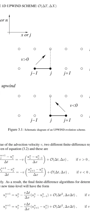
This ambiguity is the consequence of the first-order approximation which prevents a proper “centring” of the finite-difference stencil. However, and as long as we are concerned with an advection equation, this ambiguity is easily solved if we think that the differential equation will simply translate each point in the initial solution to the new positionx+v∆t over a time interval∆t. In this case, it is natural to select the points in the solution at the time-levelnthat are “upwind” of the solution at the positionj and at the time-leveln+ 1, as these are the ones causally connected with

(15)

3.1. THE 1D UPWIND SCHEME:O(∆T,∆X) 13

t or n

x or j

j

j−1

j+1

n

n+1

j

j−1

j+1

n

n+1

v<0

v>0

upwind

Figure 3.1:Schematic diagram of an UPWIND evolution scheme.

on the value of the advection velocityv, two different finite-difference representations can be given of equation (3.2) and these are

un+1_j −un j ∆t =−v _un j −unj−1 ∆x +O(∆t,∆x), ifv >0, (3.9) un+1j −unj ∆t =−v _un j+1−unj ∆x +O(∆t,∆x), ifv <0, (3.10) respectively. As a result, the final finite-difference algorithms for determing the solu-tion at the new time-level will have the form

un+1_j =unj − v∆t ∆x(u n j −unj−1) +O(∆t2,∆x∆t), ifv >0, (3.11) un+1j =unj − v∆t ∆x(u n j+1−unj) +O(∆t2,∆x∆t), ifv <0. (3.12)

(16)

More in general, for a system of linear hyperbolic equations with state vectorU

and flux-vectorF_{, the upwind scheme will take the form}

Un+1 j =U n j ± ∆t ∆x Fn_j ∓1−Fnj +O(∆t2,∆x∆t), (3.13) where the_±sign should be chosen according to whetherv >0orv <0. The logic be-hind the choice of the stencil in an upwind method is is illustrated in Fig. 1.1 where we have shown a schematic diagram for the two possible values of the advection velocity. The upwind scheme (as well as all of the others we will consider here) is an example of an explicit scheme, that is of a scheme where the solution at the new time-level

n+ 1 can be calculated explicitly from the quantities that are already known at the previous time-leveln. This is to be contrasted with an implicit scheme in which the finite-difference representations of the differential equation has, on the right-hand-side, terms at the new time-leveln+ 1. These methods require in general the solution of a number of coupled algebraic equations and will not be discussed further here.

The upwind scheme is a stable one in the sense that the solution will not have expo-nentially growing modes. This can be seen through a von Neumann stability analysis, a useful tool which allows a first simple validation of a given numerical scheme. It is important to underline that the von Neumann stability analysis is local in the sense that:

a) it does not take into account boundary effects; b) it assumes that the coefficients of

the finite difference equations are sufficiently slowly varying to be considered constant in time and space (this is a reasonable assumptions if the equations are linear). Under these assumptions, the solution can be seen as a sum of eigenmodes which at each grid point have the form

unj =ξneikxj , (3.14)

wherekis the spatial wave number andξ=ξ(k)is a complex number.

If we now consider the symbolic representation of the finite difference equation as

un+1j =T(∆tp,∆xq)unj , (3.15)

with_T(∆tp_,_∆_xq₎_{being the evolution operator of order}_p_{in time and}_q_{in space, it then}

becomes clear from (3.14) and (3.15) that the time evolution of a single eigenmode is nothing but a succession of integer powers of the complex numberξwhich is therefore named amplification factor. This naturally leads to a criterion of stability as the one for which the modulus of the amplfication factor is always less than 1, i.e.,

|ξ|2=ξξ∗≤1. (3.16)

Using (3.14) in (3.11)–(3.12) we would obtain an amplification factor

ξ= 1− |α|(1−cos(k∆x))−iαsin(k∆x), (3.17) where

α≡ v_∆∆_xt . (3.18)

Its quared modulus_|ξ|2_≡_ξξ∗_{is then}

(17)

3.1. THE 1D UPWIND SCHEME:O(∆T,∆X) 15

∆t

n+1

COURANT STABLE

COURANT UNSTABLE

n

j+1

j-1

j+1

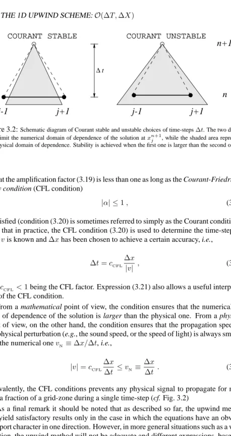
Figure 3.2:Schematic diagram of Courant stable and unstable choices of time-steps∆t. The two dashed lines limit the numerical domain of dependence of the solution atxn+1

j , while the shaded area represents

the physical domain of dependence. Stability is achieved when the first one is larger than the second one.

so that the amplification factor (3.19) is less than one as long as the

Courant-Friedrichs-L¨owy condition (CFL condition)

|α| ≤1, (3.20)

is satisfied (condition (3.20) is sometimes referred to simply as the Courant condition.). Note that in practice, the CFL condition (3.20) is used to determine the time-step∆t

oncevis known and∆xhas been chosen to achieve a certain accuracy, i.e.,

∆t=cCFL

∆x

|v| , (3.21)

withcCFL <1being the CFL factor. Expression (3.21) also allows a useful interpreta-tion of the CFL condiinterpreta-tion.

From a mathematical point of view, the condition ensures that the numerical do-main of dependence of the solution is larger than the physical one. From a physical point of view, on the other hand, the condition ensures that the propagation speed of any physical perturbation (e.g., the sound speed, or the speed of light) is always smaller than the numerical onevN ≡∆x/∆t, i.e.,

|v|=cCFL

∆x

∆t ≤vN ≡

∆x

∆t . (3.22)

Equivalently, the CFL conditions prevents any physical signal to propagate for more than a fraction of a grid-zone during a single time-step (cf. Fig. 3.2)

As a final remark it should be noted that as described so far, the upwind method will yield satisfactory results only in the case in which the equations have an obvious transport character in one direction. However, in more general situations such as a wave equation, the upwind method will not be adequate and different expressions, based on finite-volume formulations of the equations will be needed [1, 4].

(18)

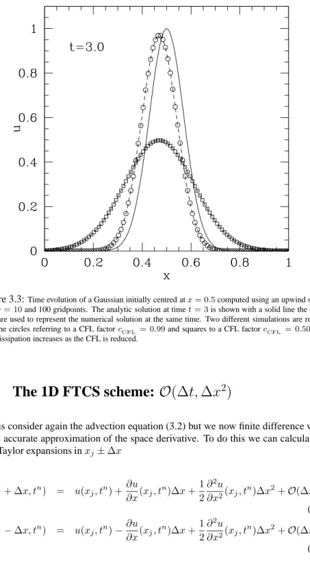
Figure 3.3:Time evolution of a Gaussian initially centred atx= 0.5computed using an upwind scheme withv= 10and 100 gridpoints. The analytic solution at timet= 3is shown with a solid line the dashed lines are used to represent the numerical solution at the same time. Two different simulations are reported with the circles referring to a CFL factorcCFL = 0.99and squares to a CFL factorcCFL = 0.50. Note

how dissipation increases as the CFL is reduced.

3.2

The 1D FTCS scheme:

O

(∆

t,

∆

x

2

)

Let us consider again the advection equation (3.2) but we now finite difference with a more accurate approximation of the space derivative. To do this we can calculate the two Taylor expansions inxj±∆x

u(xj+ ∆x, tn) = u(xj, tn) +∂u ∂x(xj, t n_)∆_x₊1 2 ∂2_u ∂x2(xj, t n_)∆_x2₊ O(∆x3), (3.23) u(xj−∆x, tn) = u(xj, tn)− ∂u ∂x(xj, t n_)∆_x₊1 2 ∂2_u ∂x2(xj, t n_)∆_x2₊ O(∆x3), (3.24)

(19)

3.2. THE 1D FTCS SCHEME:O(∆T,∆X2) 17

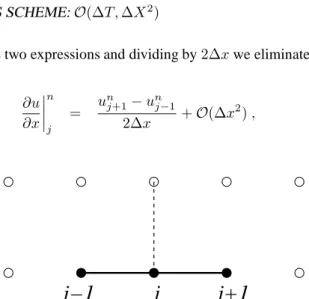
Subtracting now the two expressions and dividing by2∆xwe eliminate the first-order terms and obtain

∂u ∂x n j = u n j+1−unj−1 2∆x +O(∆x 2₎_, _(3.25)

j

j−1

j+1

FTCS

n

n+1

Figure 3.4:Schematic diagram of a FTCS evolution scheme.

Using now the second-order accurate operator (3.25) we can finite-difference equa-tion (3.2) through the so called FTCS (Forward-Time-Centered-Space) scheme in which a first-order approximation is used for the time derivative, but a second order one for the spatial one. Using the a finite-difference notation, the FTCS is then expressed as

un+1_j −un j ∆t =−v _un j+1−unj−1 2∆x +O(∆t,∆x2), (3.26) so that un+1_j =unj − α 2(u n j+1−unj−1) +O(∆t2,∆x2∆t), (3.27)

or more generically, for a system of linear hyperbolic equations

Un+1 j =Unj − ∆t 2∆x _Fn j+1−Fnj−1 +O(∆t2,∆x2∆t), (3.28) The stencil for the finite- differencing (3.27) is shown symbolically in Fig. 3.4.

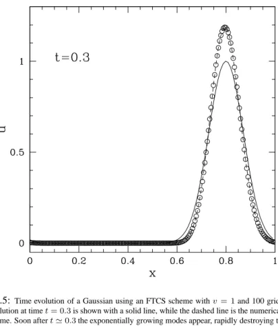
Disappointingly, the FTCS scheme is unconditionally unstable: i.e., the numerical solution will be destroyed by numerical errors which will be certainly produced and grow exponentially. This is shown in Fig. 3.5 where we show the time evolution of a Gaussian using an FTCS scheme 100 gridpoints. The analytic solution at timet= 0.3

is shown with a solid line the dashed lines are used to represent the numerical solution at the same time. Note that the solution plotted here refers to a time which is 10 times smaller than the one in Fig. 3.3. Soon aftert ≃0.3the exponentially growing modes appear, rapidly destroying the solution.

Applying the definition (3.14) to equation (3.26) and few algebraic steps lead to an amplification factor

(20)

Figure 3.5: Time evolution of a Gaussian using an FTCS scheme withv= 1and 100 gridpoints. The analytic solution at timet= 0.3is shown with a solid line, while the dashed line is the numerical solution at the same time. Soon aftert≃0.3the exponentially growing modes appear, rapidly destroying the solution.

whose squared modulus is

|ξ|2= 1 + (αsin(k∆x))2>1, (3.30) thus proving the unconditional instability of the FTCS scheme. Because of this, the FTCS scheme is rarely used and will not produce satisfactory results but for a very short timescale as compared to the typical crossing time of the physical problem under investigation.

A final aspect of the von Neumann stability worth noticing is that it is a

neces-sary but not sufficient condition for stability. In other words, a numerical scheme that

appears stable with respect to a von Neumann stability analysis might still be unstable.

3.3

The 1D Lax-Friedrichs scheme:

O

(∆

t,

∆

x

2

)

A solution to the stability problems offered by the FTCS scheme was proposed by Lax and Friedrichs. The basic idea is very simple and is based on replacing, in the FTCS

(21)

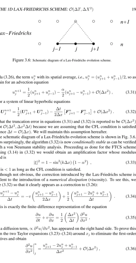
3.3. THE 1D LAX-FRIEDRICHS SCHEME:O(∆T,∆X2) 19

j

j−1

j+1

n

n+1

Lax−Friedrichs

Figure 3.6:Schematic diagram of a Lax-Friedrichs evolution scheme.

formula (3.26), the termun

j with its spatial average, i.e.,unj = (unj+1+unj−1)/2, so as

to obtain for an advection equation

un+1_j = 1 2(u n j+1+unj−1)− α 2(u n j+1−unj−1) +O(∆x2), (3.31)

and, for a system of linear hyperbolic equations

Un+1 j = 1 2(U n j+1+Unj−1)− ∆t 2∆x _Fn j+1−Fnj−1 +O(∆x2). (3.32) Note that the truncation error in equations (3.31) and (3.32) is reported to be_O(∆x2₎

and not_O(∆t2_,_∆_x2_∆_t₎_{because we are assuming that the CFL condition is satisfied}

and hence∆t=O(∆x). We will maintain this assumption hereafter.

The schematic diagram of a Lax-Friedrichs evolution scheme is shown in Fig. 3.6. Perhaps surprisingly, the algorithm (3.32) is now conditionally stable as can be verified through a von Neumann stability analysis. Proceeding as done for the FTCS scheme and using (3.14) in (3.32) we would obtain an amplification factor whose modulus squared is

|ξ|2= 1−sin2(k∆x) 1−α2

, (3.33)

which is<1as long as the CFL condition is satisfied.

Although not obvious, the correction introduced by the Lax-Friedrichs scheme is equivalent to the introduction of a numerical dissipation (viscosity). To see this, we rewrite (3.32) so that it clearly appears as a correction to (3.26):

un+1_j −un j ∆t =−v _un j+1−unj−1 2∆x +1 2 _un j+1−2unj +unj−1 ∆t . (3.34)

This is exactly the finite-difference representation of the equation

∂u ∂t +v ∂u ∂x = 1 2 ∆x2 ∆t ∂2_u ∂x2 , (3.35)

where a diffusion term,_∝∂2_u/∂x2_{, has appeared on the right hand side. To prove this}

we sum the two Taylor expansions (3.23)–(3.24) aroundxjto eliminate the first-order

derivatives and obtain

∂2_u ∂x2 n j =u n j+1−2unj +unj−1 ∆x2 +O(∆x 2₎_, _(3.36)

(22)

where the sum has allowed us to cancel both the terms_O(∆x)and_O(∆x3₎_{. Note}

that since the expression for the second derivative in (3.36) is_O(∆x2₎_{, it is appears}

multiplied by∆x2_/_∆_t ₌_O_(∆_x₎_{in equation (3.35), thus making the right-hand-side}

O(∆x3₎_{overall. The left-hand-side, on the other hand, is only}_O_(∆_x₎_{(the time}

deriva-tive is_O(∆x), while the spatial derivative is_O(∆x2₎_{). As a result, the dissipative}

term goes to zero more rapidly than the intrinsic truncation error of the Lax-Friedrichs scheme, thus guaranteeing that the in the continuum limit the algorithm will converge to the correct solution of the advection equation.

Figure 3.7:This is the same as in Fig. 3.3 but for a Lax-Friedrichs scheme. Note how the scheme is stable but also suffers from a considerable dissipation.

A reasonable objection could be made for the fact that the Lax-Friedrichs scheme has changed the equation whose solution one is interested in [i.e., eq. (3.2)] into a new equation, in which a spurious numerical dissipation has been introduced [i.e., eq. (3.35)]. Unless_|v|∆t = ∆x,_|ξ| < 1 and the amplitude of the wave is doomed to decrease (see Fig. 3.7).

However, such objection can be easily circumvented. As mentioned above, the dissipative term is always smaller than the truncation error thus guaranteeing the con-vergence to the correct solution. Furthermore, it is useful to bear in mind that the key

(23)

3.4. THE 1D LEAPFROG SCHEME:O(∆T2,∆X2) 21

aspect in any numerical representation of a physical phenomenon is the determination of the length scale over which we need to achieve an accurate description. In a finite difference approach, this length scale must necessarily encompass many grid points and for which k∆x ≪ 1. In this case, expression (3.33) clearly shows that the am-plification factor is very close to 1 and the effects of dissipation are therefore small. Note that this is true also for the FTCS scheme so that on these scales the stable and unstable schemes are equally accurate. On the very small scales however, which we are not of interest to us,k∆x∼1and the stable and unstable schemes are radically dif-ferent. The first one will be simply inaccurate, the second one will have exponentially growing errors which will rapidly destroy the whole solution. It is rather obvious that stability and inaccuracy are by far preferable to instability, especially if the accuracy is lost over wavelengths that are not of interest or when it can be recovered easily by using more refined grids. This is called “consistency” of the discretized operator and will be discussed in detail in Sect. 4.2.2.

3.4

The 1D Leapfrog scheme:

O

(∆

t

2

,

∆

x

2

)

Both the FTCS and the Lax-Friedrichs are “one-level” schemes with first-order ap-proximation for the time derivative and a second-order apap-proximation for the spatial derivative. In those circumstancesv∆tshould be taken significantly smaller than∆x

(to achieve the desired accuracy), well below the limit imposed by the Courant condi-tion.

j−1

j+1

n

n+1

Leapfrog

n−1

j

Figure 3.8:Schematic diagram of a Leapfrog evolution scheme.

Second-order accuracy in time can be obtained if we insert

∂u ∂t n j = u n+1 j −u n−1 j 2∆t +O(∆t 2₎_, _(3.37)

in the FTCS scheme, to find the Leapfrog scheme

un+1_j =un−1

j −α unj+1−unj−1

(24)

where it should be noted that the factor 2 in∆xcancels the equivalent factor 2 in∆t.

Figure 3.9: This is the same as in Fig. 3.3 but for a Leapfrog scheme. Note how the scheme is stable and does not suffers from a considerable dissipation even for low CFL factors. However, the presence of a little “dip” in the tail of the Gaussian for the case ofcCFL= 0.5is the result of the dispersive nature of the

numerical scheme.

For a set of linear equations, the Leapfrog scheme simply becomes

Un+1 j =Unj−1− ∆t ∆x _Fn j+1−Fnj−1 +O(∆x2), (3.39) and the schematic diagram of a Leapfrog evolution scheme is shown in Fig. 3.8.

Also for the case of a Leapfrog scheme there are a number of aspects that should be noticed:

• In a Leapfrog scheme that is Courant stable, there is no amplitude dissipation (i.e.,_|ξ|2_{= 1}_{). In fact, a von Neumann stability analysis yields}

ξ=−iαsin(k∆x)± q 1−[αsin(k∆x)]2, (3.40) and so that |ξ|2₌_α2_sin2₍_k_∆_x_{) +}_{₁₋_[_α_sin(_k_∆_x_)]2 }= 1 ∀α≤1. (3.41)

(25)

3.5. THE 1D LAX-WENDROFF SCHEME:O(∆T2,∆X2) 23

n+1

n-1

n

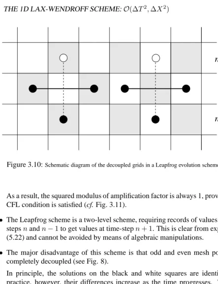
Figure 3.10:Schematic diagram of the decoupled grids in a Leapfrog evolution scheme.

As a result, the squared modulus of amplification factor is always 1, provided the CFL condition is satisfied (cf. Fig. 3.11).

• The Leapfrog scheme is a two-level scheme, requiring records of values at time-stepsnandn−1to get values at time-stepn+ 1. This is clear from expression (5.22) and cannot be avoided by means of algebraic manipulations.

• The major disadvantage of this scheme is that odd and even mesh points are completely decoupled (see Fig. 8).

In principle, the solutions on the black and white squares are identical. In practice, however, their differences increase as the time progresses. This ef-fect, which becomes evident only on timescales much longer then the crossing timescale, can be cured either by discarding one of the solutions or by adding a dissipative term of the type

. . .+ǫ(un

j+1−2unj+1+unj+1), (3.42)

in the right-hand-side of (5.17), whereǫ≪1is an adjustable coefficient.

3.5

The 1D Lax-Wendroff scheme:

O

(∆

t

2

,

∆

x

2

)

The Lax-Wendroff scheme is the second-order accurate extension of the Lax-Friedrichs scheme. As for the case of the Leapfrog scheme, in this case too we need two time-levels to obtain the solution at the new time-level.

There are a number of different ways of deriving the Lax-Wendroff scheme but it is probably useful to look at it as to a combination of the Lax-Friedrichs scheme and of the Leapfrog scheme. In particular a Lax-Wendroff scheme can be obtained as

(26)

1. A Lax-Friedrichs scheme with half step: Un+ 1 2 j+1 2 = 1 2 _Un j+1+U n j −_2∆∆t_x_Fn j+1−F n j +O(∆x2), Un+ 1 2 j−1 2 =1 2 _Un j +Unj−1 −_2∆∆t_x_Fn j −Fnj−1 +O(∆x2),

where∆t/(2∆x)comes from having used a timestep∆t/2;

2. The evaluation of the fluxesFn+

1 2

j±1 2

from the values ofUn+

1 2 j±1 2 3. A Leapfrog “half-step”: Un+1 j =U n j − ∆t ∆x h Fn+ 1 2 j+1 2 − Fn+ 1 2 j−1 2 i +O(∆x2). (3.43)

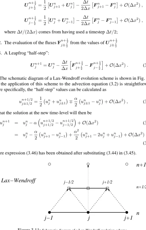
The schematic diagram of a Lax-Wendroff evolution scheme is shown in Fig. 3.11 and the application of this scheme to the advection equation (3.2) is straightforward. More specifically, the “half-step” values can be calculated as

un+1/2_j_±_1/2 = 1 2 u n j +uuj±1 ∓α₂ unj±1−unj +O(∆x2), (3.44) so that the solution at the new time-level will then be

un+1j = unj −α un+1/2_j+1/2 −un+1/2_j₋_1/2+O(∆x2) (3.45) = unj − α 2 u n j+1−unj−1 +α 2 2 u n j+1−2unj +unj−1 +O(∆x2). (3.46) where expression (3.46) has been obtained after substituting (3.44) in (3.45).

n+1

n

j−1

j

j+1

n+1/2 j+1/2 j−1/2

Lax−Wendroff

Figure 3.11:Schematic diagram of a Lax-Wendroff evolution scheme.

(27)

3.6. THE 1D ICN SCHEME:O(∆T2,∆X2) 25

• In the Lax-Wendroff scheme there might be some amplitude dissipation. In fact, a von Neumann stability analysis yields

ξ= 1−iαsin(k∆x)−α2[1−cos(k∆x)] , (3.47) so that the squared modulus of the amplification factor is

|ξ|2= 1−α2(1−α2)

1−cos2(k∆x)

. (3.48)

As a result, the von Neumann stability criterion_|ξ|2 _≤ ₁ _{is satisfied as long}

asα2 _≤ ₁_{, or equivalently, as long as the CFL condition is satisfied. (cf. Fig.}

10). It should be noticed, however, that unlessα2 _{= 1}_{, then}_|_ξ_|2 _<₁_{and some}

amplitude dissipation is present. In this respect, the dissipative properties of the Lax-Friedrichs scheme are not completely lost in the Lax-Wendroff scheme but are much less severe (cf. Figs. 5 and 10).

• The Lax-Wendroff scheme is a two-level scheme, but can be recast in a one-level form by means of algebraic manipulations. This is clear from expressions (3.46) where quantities at time-levelsnandn+ 1only appear.

3.6

The 1D ICN scheme:

O

(∆

t

2

,

∆

x

2

)

The idea behind the iterative Crank-Nicolson (ICN) scheme is that of transforming a stable implicit method, i.e., the Crank-Nicolson (CN) scheme (see Sect. 8.4.2) into an explicit one through a series of iterations. To see how to do this in practice, consider differencing the advection equation (3.2) having a centred space derivative but with the time derivative being backward centred, i.e.,

un+1j −unj ∆t =−v un+1j+1 −un+1j−1 2∆x ! . (3.49)

This scheme is also known as “backward in time, centred in space” or BTCS (see Sect. 8.4.1) and has amplification factor

ξ= 1

1 + iαsink∆x, (3.50)

so that_|ξ|2_<₁_{for any choice of}_α_{, thus making the method unconditionally stable.}

The Crank-Nicolson (CN) scheme, instead, is a second-order accurate method ob-tained by averaging a BTCS and a FTCS method or, in other words, equations (3.26) and (3.49). Doing so one then finds

ξ=1 + iαsink∆x/2

1−iαsink∆x/2 . (3.51)

so that the method is stable. Note that although one averages between an explicit and an implicit scheme, terms containingun+1_{survive on the right hand side of equation}

(28)

Figure 3.12: This is the same as in Fig. 3.3 but for a Lax-Wendroff scheme. Note how the scheme is stable and does not suffers from a considerable dissipation even for low CFL factors. However, the presence of a little “dip” in the tail of the Gaussian for the case ofcCFL= 0.5is the result of the dispersive nature of

the numerical scheme.

The first iteration of iterative Crank-Nicolson starts by calculating an intermediate variable(1)u˜using equation (3.26):

(1)_u_˜n+1 j −unj ∆t =−v _un j+1−unj−1 2∆x . (3.52)

Then another intermediate variable(1)u¯is formed by averaging:

(1)_u_¯n+1/2 j ≡ 1 2 (1)_u_˜n+1 j +unj . (3.53)

Finally the timestep is completed by using equation (3.26) again withu¯on the right-hand side: un+1_j −un j ∆t =−v (1)_u_¯n+1/2 j+1 −(1)u¯ n+1/2 j−1 2∆x ! . (3.54)

(29)

3.6. THE 1D ICN SCHEME:O(∆T2,∆X2) 27

Iterated Crank-Nicolson with two iterations is carried out in much the same way. After steps (3.52) and (3.53), we calculate

(2)_u_˜n+1 j −unj ∆t = −v (1)_u_¯n+1/2 j+1 −(1)u¯ n+1/2 j−1 2∆x ! , (3.55) (2)_u_¯n+1/2 j ≡ 1 2 (2)_u_˜n+1 j +unj . (3.56)

Then the final step is computed analogously to equation (3.54):

un+1_j −un j ∆t =−v (2)_u_¯n+1/2 j+1 −(2)u¯ n+1/2 j−1 2∆x ! . (3.57)

Further iterations can be carried out following the same logic.

To investigate the stability of these iterated schemes we compute the amplification factors relative to the different iterations to be

(1)_ξ _{= 1 + 2i}_{β ,} _(3.58) (2)_ξ _{= 1 + 2i}_β −2β2, (3.59) (3)_ξ _{= 1 + 2i}_β −2β2−2iβ3, (3.60) (4)_ξ _{= 1 + 2i}_β₋₂_β2₋_2i_β3_{+ 2}_β4_, _(3.61)

whereβ ≡ (α/2) sin(k∆x), and(1)ξ corresponds to the FTCS scheme. Note that the amplification factors (3.58) correspond to those one would obtain by expanding equation (3.51) in powers ofβ.

Computing the squared moduli of (3.58) one encounters an alternating and recur-sive pattern. In particular, iterations 1 and 2 are unstable (_|ξ|2_>₁_{); iterations 3 and 4}

are stable (_|ξ|2_<₁_{) provided}_β2_≤₁_{; iterations 5 and 6 are also unstable; iterations 7}

and 8 are stable providedβ2 _≤₁_{; and so on. Imposing the stability for all}

wavenum-bersk, we obtainα2_/₄_≤₁_{, or}_∆_t_≤_2∆_x_{which is just the CFL condition [the factor}

2 is inherited by the factor 2 in equation (3.26)].

In other words, while the magnitude of the amplification factor for iterated Crank-Nicolson does approach 1 as the number of iterations becomes infinite, the convergence is not monotonic. The magnitude oscillates above and below 1 with ever decreasing os-cillations. All the iterations leading to_|ξ|2_{above 1 are unstable, although the instability}

might be very slowly growing as the number of iterations increases. Because the trun-cation error is not modified by the number of iterations and is always_O(∆t2,∆x2), a number of iterations larger than two is never useful; three iterations, in fact, would simply amount to a larger computational cost.

3.6.1

ICN as a

θ

-method

In the ICN method theM-th average is made weighting equally the newly predicted solution(M)u˜n+1_j and the solution at the “old” timelevel”un_{. This, however, can be}

seen as the special case of a more generic averaging of the type

(30)

where0< θ <1is a constant coefficient. Predictor-corrector schemes using this type of averaging are part of a large class of algorithms namedθ-methods [10], and we refer

to the ICN generalized in this way as to the “θ-ICN” method.

A different and novel generalization of theθ-ICN can be obtained by swapping the averages between two subsequent corrector steps, so that in theM-th corrector step

(M)_u_¯n+1/2_{= (1}₋_θ₎(M)_u_˜n+1₊_θun_, _(3.63)

while in the(M + 1)-th corrector step

(M+1)_u_¯n+1/2₌_θ(M+1)_u_˜n+1_{+ (1}

−θ)un. (3.64)

Note that as long as the number of iterations is even, the sequence in which the aver-ages are computed is irrelevant. Indeed, the weightsθand1−θin eqs. (3.63)–(3.64) could be inverted and all of the relations discussed hereafter for the swapped weighted averages would continue to hold after the transformationθ→1−θ.

Constant Arithmetic Averages

Using a von Neumann stability analysis, Teukolsky has shown that for a hyperbolic equation the ICN scheme withMiterations has an amplification factor [13]

(M)_ξ_{= 1 + 2} M X n=1

(−iβ)n , (3.65)

whereβ ≡v[∆t/(2∆x)] sin(k∆x)1_{. More specifically, zero and one iterations yield}

an unconditionally unstable scheme, while two and three iterations a stable one pro-vided thatβ2_≤₁_{; four and five iterations lead again to an unstable scheme and so on.}

Furthermore, because the scheme is second-order accurate from the first iteration on, Teukolsky’s suggestion when using the ICN method for hyperbolic equations was that two iterations should be used and no more [13]. This is the number of iterations we will consider hereafter.

Constant Weighted Averages

Performing the same stability analysis for aθ-ICN is only slightly more complicated and truncating at two iterations the amplification factor is found to be

ξ= 1−2iβ−4β2θ+ 8iβ3θ2 , (3.66) whereξ is a shorthand for (2)ξ. The stability condition in this case translates into requiring that

16β4θ4−4β2θ2−2θ+ 1≤0, (3.67) or, equivalently, that forθ >3/8

r 1 2− q 2θ−34 2θ ≤β≤ r 1 2+ q 2θ−34 2θ , (3.68)

(31)

3.6. THE 1D ICN SCHEME:O(∆T2,∆X2) 29

Figure 3.13: Left panel: stability region in the (θ, β) plane for the two-iterationsθ-ICN for the advection equation (3.2). Thick solid lines mark the limit at which_|ξ| = 1, while the dotted contours indicate the values of the amplification factor in the stable region. The shaded area forθ <1/2refers to solutions that are linearly unstable [15].

Right panel: same as in the left panel but when the averages between two corrections

are swapped. Note that the amplification factor in this case is less sensitive onθand always larger than the corresponding amplification factor in the left panel.

which reduces to β2 _≤ ₁ _when _θ _{= 1}_/₂_{. Because the condition (3.68) must hold}

for every wavenumberk, we consider hereafterβ ≡v∆t/(2∆x)and show in the left panel of Fig. 3.13 the region of stability in the (θ, β) plane. The thick solid lines mark the limit at which_|ξ|= 1, while the dotted contours indicate the different values of the amplification factor in the stable region.

A number of comments are worth making. Firstly, although the condition (3.68) allows for weighting coefficientsθ <1/2, theθ-ICN is stable only ifθ ≥ 1/2. This is a known property of the weighted Crank-Nicolson scheme [10] and inherited by the

θ-ICN. In essence, whenθ 6= 1/2 spurious solutions appear in the method [16] and these solutions are linearly unstable ifθ <1/2, while they are stable forθ >1/2[15]. For this reason we have shaded the area withθ < 1/2 in the left panel of Fig. 3.13 to exclude it from the stability region. Secondly, the use of a weighting coefficient

θ >1/2will still lead to a stable scheme provided that the timestep (i.e.,β) is suitably decreased. Finally, as the contour lines in the left panel of Fig. 3.13 clearly show, the amplification factor can be very sensitive onθ.

Swapped weighted averages

The calculation of the stability of theθ-ICN when the weighted averages are swapped as in eqs. (3.63) and (3.64) is somewhat more involved; after some lengthy but

(32)

straight-forward algebra we find the amplification factor to be

ξ = 1−2iβ−4β2_θ_{+ 8i}_β3_θ₍₁₋_θ₎_, _(3.69)

which differs from (3.66) only in that theθ2_{coefficient of the}_O₍_β3₎_{term is replaced}

byθ(1−θ). The stability requirement_|ξ| ≤1is now expressed as

16β4θ2(1−θ)2−4β2θ(2−3θ)−2θ+ 1≤0. (3.70) Solving the condition (3.70) with respect toβamounts then to requiring that

β ≥ p 2−3θ−√4θ−11θ2_{+ 8}_θ3 2(1−θ)√2θ , (3.71a) β ≤ p 2−3θ+√4θ−11θ2_{+ 8}_θ3 2(1−θ)√2θ , (3.71b)

which is again equivalent to β2 _≤ ₁ _when_θ _{= 1}_/₂_{. The corresponding region of}

stability is shown in right panel of Fig. 3.13 and should be compared with left panel of the same Figure. Note that the average-swapping has now considerably increased the amplification factor, which is always larger than the corresponding one for theθ-ICN in the relevant region of stability (i.e., for1/2≤θ≤12_).

2_{Of course, when the order of the swapped averages is inverted from the one shown in eqs. (3.63)–(3.64)}

(33)

3.6. THE 1D ICN SCHEME:O(∆T2,∆X2) 31

3.6.2

Summary

In what follow I summarize the most salient aspects of the different finite-difference operators discussed so far and report, for each of them, the truncation errorǫT, the amplification factor_|ξ|2_{and the finite-difference representation of the advection}

equa-tion 3.2.

Method ǫT |ξ|

2 _for ₍_k_∆_x_≪₁₎ _{finite-difference form}

Upwind _O(∆t,∆x) 1−2|α|(1− |α|) cos(k∆x) un+1j =unj ∓α(unj±1−unj)

FTCS _O(∆t,∆x2₎ _{1 + sin}2₍_k_∆_x₎_α2 _un+1

j =unj −α(unj+1−unj−1)

Lax Friedrichs _O(∆t,∆x2₎ ₁₋_sin2₍_k_∆_x₎₍₁

−α2₎ _un+1 j = 12(u n j+1+unj−1)− α(un j+1−unj−1) Lepafrog _O(∆t2_,_∆_x2₎ ₁ _un+1 j =u n−1 j −α(unj+1−unj−1)

Lax Wendroff _O(∆t2_,_∆_x2₎ ₁₋_α2₍₁₋_α2_{) sin}2₍_k_∆_x₎ _un+1

j =unj −12α(u n j+1−unj−1)− 1 2α 2₍_un j+1−2unj +unj−1)

(34)

3.6.3

Finite-difference stencils

In what follow I summarize the most used finite-difference stencils for derivatives of order1to4

Finite difference stencils for∂u_/∂x

type Difference Stencil LTE

forward (−uj+uj+1)/h O(h) backward (−uj−1+uj)/h O(h) forward (−3uj+ 4uj+1−uj+2)/h O(h2) backward (uj−2−4uj−1+ 3uj)/2h O(h2) centered (−uj−1+uj+1)/2h O(h2) forward (−25uj+ 48uj+1−36uj+2+ 16uj+3−3uj+4)/12h O(h4) backward (3uj−4−16uj−3+ 36uj−2−48uj−1+ 25uj)/12h O(h4) centered (uj−2−8uj−1+ 8uj+1−uj+2)/12h O(h4)

Table 3.2:Finite difference stencils for∂u/∂x

Finite difference stencils for∂2_u

(35)

3.6. THE 1D ICN SCHEME:O(∆T2,∆X2) 33

forward (uj−2uj+1+uj+2)/h2 O(h) backward (uj−2−2uj−1+uj)/h2 O(h) forward (2uj−5uj+1+ 4uj+2−uj+3)/h2 O(h2) backward (−uj−3+ 4uj−2−5uj−1+ 2uj)/h2 O(h2) centered (uj−1−2uj+uj+1)/h2 O(h2) forward (45uj−154uj+1+ 214uj+2−156uj+3+ 61uj+4−10uj+5)/12h2 O(h4) backward (−10uj−5+ 61uj−4−156uj−3+ 214uj−2−154uj−1+ 45uj)/12h2 O(h4) centered (−uj−2+ 16uj−1−30uj+ 16uj+1−uj+2)/12h2 O(h4)

Table 3.3:Finite difference stencils for∂2_u/∂2_x

Finite difference stencils for∂3_u

/∂3_x Finite difference stencils for∂4_u

(36)

type Difference Stencil LTE forward (−uj+ 3uj+1−3uj+2+uj+3)/h3 O(h) backward (−uj−3+ 3uj−2−3uj−1+uj)/h3 O(h) forward (−5uj+ 18uj+1−24uj+2+ 14uj+3−3uj+4)/2h3 O(h2) backward (3uj−4−14uj−3+ 24uj−2−18uj−1+ 5uj)/2h3 O(h2) centered (−uj−2+ 2uj−1−2uj+1+uj+2)/2h3 O(h2)

Table 3.4:Finite difference stencils for∂3

u/∂3

x

forward (uj−4uj+1+ 6uj+2−4uj+3+uj+4)/h4 O(h)

backward (uj−4−4uj−3+ 6uj−2−4uj−1+uj)/h4 O(h)

forward (3uj−14uj+1+ 26uj+2−24uj+3+ 11uj+4−2uj+5)/h4 O(h2)

backward (−2uj−5+ 11uj−4−24uj−3+ 26uj−2−14uj−1+ 3uj)/h4 O(h2)

centered (uj−2−4uj−1+ 6uj−4uj+1+uj+2)/h4 O(h2)

Table 3.5:Finite difference stencils for∂4

u/∂4

(37)

Chapter 4

Dissipation, Dispersion and

Convergence

We will here discuss a number of problems that often emerge when using finite-difference techniques for the solution of hyperbolic partial differential equations. In stable numer-ical schemes the impact of many of these problems can be suitably reduced by going to sufficiently high resolutions, but it is nevertheless important to have a simple and yet clear idea of what are the most common sources of these problems.

4.1

On the Origin of Dissipation and Dispersion

We have already seen in Chapter 3 how the Lax-Friedrichs scheme applied to a linear advection equation (3.2) yields the finite-difference expression

un+1_j = 1 2(u n j+1+unj−1)− α 2(u n j+1−unj−1) +O(∆x2). (4.1)

We have also mentioned how expression (4.1) can be rewritten as

un+1j =unj − α 2(u n j+1−unj−1) + 1 2(u n j+1−2unj +unj−1) +O(∆x2), (4.2)

to underline how the Lax-Friedrichs scheme effectively provides a first-order finite-difference representation of a non-conservative equation

∂u ∂t +v ∂u ∂x =εLF ∂2_u ∂x2 , (4.3)

that is an advection-diffusion equation in which a dissipative term

εLF≡v

∆x2

2∆t , (4.4)

is present. Given a computational domain of lengthL, this scheme will therefore have a typical diffusion timescaleτ ≃L2_/ε

LF. Clearly, the larger the diffusion coefficient, the faster will the solution be completely smeared over the computational domain.

(38)

In a similar way, it is not difficult to realize that the upwind scheme

un+1_j =unj −α unj −unj−1

+O(∆x2), (4.5)

provides a first-order accurate (in space) approximation to equation (3.2), but a second-order approximation to equation

∂u ∂t +v ∂u ∂x =εUW ∂2_u ∂x2 , (4.6) where εUW ≡ v∆x 2 . (4.7)

Stated differently, also the upwind method reproduces at higher-order an advection-diffusion equation with a dissipative term which is responsible for the gradual dissi-pation of the advected quantityu. This is shown in Fig. 4.2 for a wave packet (i.e., a periodic function embedded in a Gaussian) propagating to the right and where it is important to notice how the different peaks in the packet are advected at the correct speed, although their amplitude is considerably diminished.

In Courant-limited implementations,α =|v|∆t/∆x < 1so that the ratio of the dissipation coefficients can be written as

εLF

εUW

= 1

α≥1, for α∈[0,1]. (4.8)

In other words, while the upwind and the Lax-Friedrichs methods are both dissipative, the latter is generically more dissipative despite being more accurate in space. This can be easily appreciated by comparing Figs. 3.3 and 3.7 but also provides an important rule: a more accurate numerical scheme is not necessarily a preferable one.

A bit of patience and a few lines of algebra would also show that the Lax-Wendroff scheme for the advection equation (3.2) [cf. eq. (3.46)]

un+1j =unj −α unj+1−unj−1 +α 2 2 u n j+1−2unj +unj−1 +O(∆x2). (4.9) provides a first-order accurate approximation to equation (3.2), a second-order approx-imation to an advection-diffusion equation with dissipation coefficientεLW, and a third-order approximation to equation

∂u ∂t +v ∂u ∂x =εLW ∂2_u ∂x2 +βLW ∂3_u ∂x3 , (4.10) where εLW ≡ αv∆x 2 , βLW ≡ − v∆x2 6 1−α 2 . (4.11)

As mentioned in Section 3, the Lax-Wendroff scheme retains some of the dissi-pative nature of the originating Lax-Friedrichs scheme and this is incorporated in the dissipative term proportional toεLW. Using expression (4.9), it is easy to deduce the

(39)

4.1. ON THE ORIGIN OF DISSIPATION AND DISPERSION 37

Figure 4.1:Time evolution of a wave-packet initially centred atx= 0.5computed using a Lax-Friedrichs scheme withCCFL= 0.75. The analytic solution at timet= 2is shown with a solid line the dashed lines

are used to represent the numerical solution at the same time. Note how dissipation reduces the amplitude of the wave-packet but does not change sensibly the propagation of the wave-packet.

magnitude of this dissipation and compare it with the equivalent one produced with the Lax-Friedrichs scheme. A couple of lines of algebra show that

εLW =α

2_ε

LF ≪εLF, (4.12)

thus emphasizing that the Lax-Wendroff scheme is considerably less dissipative than the corresponding Lax-Friedrichs.

The simplest way of quantifying the effects introduced by the right-hand-sides of equations (4.3), (4.6), and (4.10) is by using a single Fourier mode with angular fre-quencyωand wavenumberk, propagating in the positivex-direction, i.e.,

u(x, t) =ei(kx−ωt). (4.13)

It is then easy to verify that in the continuum limit

∂u ∂t =−iωu , ∂u ∂x = iku , ∂2_u ∂x2 =−k 2_{u ,} ∂3u ∂x3 =−ik 3_{u .} _(4.14)

(40)

Figure 4.2:Time evolution of a wave-packet initially centred atx= 0.5computed using a Lax-Wendroff scheme withCCFL = 0.75. The analytic solution at timet= 2is shown with a solid line the dashed lines

are used to represent the numerical solution at the same time. Note how the amplitude of the wave-packet is not drastically reduced but the group velocity suffers from a considerable error.

In the case in which the finite difference scheme provides an accurate approxima-tion to a purely advecapproxima-tion equaapproxima-tion, the relaapproxima-tions (4.14) lead to the obvious dispersion relationω=vk, so that the numerical modeu˜(x, t)will have a solution

˜

u(x, t) =eik(x−vt), (4.15)

representing a mode propagating with phase velocitycp≡ω/k =v, which coincides

with the group velocitycg≡∂ω/∂k=v.

However, it is simple to verify that the advection-diffusion equation approximated by the Lax-Friedrichs scheme (4.3), will have a corresponding solution

˜

u(x, t) =e−εLFk2t_eik(x−vt)_, _(4.16) thus having, besides the advective term, also an exponentially decaying mode. Simi-larly, a few lines of algebra are sufficient to realize that the dissipative term does not couple with the advective one and, as a result, the phase and group velocities remain

(41)

4.2. MEASURING DISSIPATION AND CONVERGENCE 39 the same and cp =cg = v. This is clearly shown in Fig. 4.1 which shows how the

wave packet is sensibly dissipated but, overall, maintains the correct group velocity. Finally, it is possible to verify that the advection-diffusion equation approximated by the Lax-Wendroff scheme (4.10), will have a solution given by

˜

u(x, t) =e−εLWk2t_eik[x−(v+βLWk2)t]

, (4.17)

where, together with the advective and (smaller) exponentially decaying modes already encountered before, there appears also a dispersive term_∼βLWk

2_t_{producing different}

propagation speeds for modes with different wavenumbers. This becomes apparent after calculating the phase and group velocities which are given by

cp= ω k =v+βLWk 2_, _and _c g= ∂ω ∂k =v+ 3βLWk 2_, _(4.18)

and provides a simple interpretation of the results shown in Fig. 4.2.

4.2

Measuring Dissipation and Convergence

From what discussed so far it appears clear that one is often in the need of tools that allow a rapid comparison among different evolution schemes. One might be interested, for instance, in estimating which of two methods is less dissipative or whether an evo-lution scheme which is apparently stable will eventually turn out to be unstable. In what follows we discuss some of these tools and how they can be used to ascertain a fundamental property of the numerical solution: its convergence

4.2.1

The summarising power of norms

A very useful tool that can be used in this context is the calculation of the “norms” of the quantity we are interested in. In the continuum limit the p-norm is defined as

kukp= 1 (b−a) Z b a | u(x, t)|pdx !1/p . (4.19)

and has the same dimensions of the originating quantityu(x, t). The extension of this concept to a discretised space and time is straightforward and yields the commonly used norms 1−norm :: ||u||(tn_{) =} 1 N N X j=1 |un j|, (4.20) 2−norm :: ||u||2(tn) = 1 N   N X j=1 (unj)2   1/2 , (4.21) p−norm :: ||u||p(tn) = 1 N   N X j=1 (unj)p   1/p , (4.22) infinity−norm :: ||u||∞(t n_{) = maxj=1,...N}₍_|_un j|). (4.23)

(42)

In the case of a scalar wave equation (see Sect. 5 for a discussion), the 2-norm has a physical interpretation and could be associated to the amount of energy contained in the numerical domain; its conservation is therefore a clear signature of a non-dissipative numerical scheme.

Figure 4.3:Time evolution of the logarithm of the 2-norms for the different numerical schemes discussed so far. Sommerfeld outgoing boundary conditions were used in this example.

Fig. 4.2 compares the 2-norms for the different numerical schemes discussed so far and in the case in which Sommerfeld outgoing boundary conditions were used. Note how the FTCS scheme is unstable and that the errors are already comparable with the solution well before a crossing time. Similarly, it is evident that the use of Sommerfeld boundary conditions allows a smooth evacuation of the energy in the wave from the numerical grid aftert∼6.

4.2.2

Consistency and Convergence

Consider therefore a PDE of the type

(43)

4.2. MEASURING DISSIPATION AND CONVERGENCE 41 where_Lis a second-order differential quasi-linear operator [cf. eq. (1.1)]. Let also L∆ be the discretized representation of such continuum differential operator andǫ= O(∆xp_,_∆_tq₎_{the associated truncation error, i.e.,}

L∆(u

n

i)−fin= 0 +O(∆xp,∆tq). (4.25)

For compactness let us assume that largest contribution to the truncation error can be expressed simply asǫ = Chp ₌_O₍_hp₎_where_h_{corresponds to either the spatial or}

time discretization andCis a real constant coefficient. The finite-difference represen-tation_L∆ is said to be consistent if

lim

h→0ǫ= 0, (4.26)

Letu(x, t)represent the exact solution to a PDE andu˜the exact solution of the finite-difference equation that approximates the PDE with a truncation error_O(∆xp_,_∆_tq₎_.

The finite-difference equation is said to be convergent when the truncation error tends to zero as a power ofpin∆xand a power ofqin∆t, namely

lim

h→0ǫ= ∆x

p_{+ ∆}_tq _, _(4.27)

Note that this condition is much more severe that the simple requirement that the trun-cation error will tend to zero as∆xand∆ttend to zero. The latter condition, in fact, does not ensure that the numerical solution is approaching the exact one at the expected rate, that is the rate determined by the truncation error and consequent to the choice of the given finite-difference representation of the continuum differential operator.

Since checking convergence essentially amounts to measuring how the truncation error changes with resolution, it is useful to define a local (i.e., pointwise) deviation from the exact solutionuatx=xias

ǫj(h) =u(h)_j −u(xj) (4.28)

be the magnitude of the largest truncation error (and which could be either in space or in time) associated to the numerical solutionu(h)j obtained with grid spacingh. If the

numerical method used is p-th order accurate, then

ǫj(h) =Chp +O(hp+1), (4.29)

whereCis a constant real coefficient. A different solution computed with a grid spac-ingkwill have at the same spatial positionxj a corresponding truncationǫj(k)error,

so that error ratio will be

Rj(h, k)≡ǫ_ǫj_j((h_k)₎ , (4.30) and the “numerical” local convergence order, that is the order of convergence as mea-sured from the two numerical solutions atxjwill be

˜

(44)

In the rather common case in whichk=h/2, expressions (4.30) reduces to

Rj(h, h/2) = 2p˜,

and the overall order of accuracy is measured numerically asp˜= log2(R). As we will

discuss in the following Section, the discrete representation of the continuum equations

is said to be convergent if and only ifp˜=p, i.e., if

lim h→0p˜≡

log(ǫ)

log(Ch) =p . (4.32)

Stated differently, convergence requires not only that the error is decreasing and thus that the method is consistent (see Sect. 4.2.3) but that it is decreasing at the expected

rate.

In general there will be a minimun resolution, sayhmin, below which the truncation error will dominate over the others, e.g., round-off error. Clearly, one should expect convergence only forh < hminand the solution in this case is said to be in a convergent

regime.

What discussed so far assumes the knowledge of the exact solution, which, in gen-eral, is not available. This does not represent a major obstacle and the convergence test can still be performed by simply employing a third numerical evaluation of the solution. This is referred to as a “self-convergence” test and exploits the fact that the difference between two numerical solutions does not depend on the actual exact solution

u(h)_j −u(k)_j =ǫj(h)−u(xj)−ǫj(k)−u(xj)

=ǫj(h)−ǫj(k),

where of course the two solutionsu(h)j andu (k)

j should be evaluated at the same

grid-pointxj. If one of the numerical solutions is not availble at such a point (e.g., because

the spacing used is not uniform) a suitable interpolation is needed and attention must be paid that the error it introduces is much smaller than eitherǫj(h)orǫj(k)in order

not to spoil the convergence test.

With (4.29) in mind and using three different numer