Optical Spatial Division Multiplexing
Downloaded from: https://research.chalmers.se, 2019-05-11 11:51 UTC
Citation for the original published paper (version of record):
Yan, L., Fiorani, M., Muhammad, A. et al (2018)
Network Performance Trade-Off in Modular Data Centers With Optical Spatial Division Multiplexing
Journal of Optical Communications and Networking, 10(9): 796-808
http://dx.doi.org/10.1364/JOCN.10.000796
N.B. When citing this work, cite the original published paper.
research.chalmers.se offers the possibility of retrieving research publications produced at Chalmers University of Technology. It covers all kind of research output: articles, dissertations, conference papers, reports etc. since 2004.
research.chalmers.se is administrated and maintained by Chalmers Library
Network Performance Trade-Off in Modular Data
Centers With Optical Spatial Division Multiplexing
Li Yan, Matteo Fiorani, Ajmal Muhammad, Massimo Tornatore,
Erik Agrell, and Lena Wosinska
Abstract—The modular design based on spatial division multi-plexing switches is recently proposed to improve the capacity and reduce the cabling complexity of data center networks. However, due to the coexistence of mice and elephant flows, in modular data center networks a trade-off between the blocking probability and total throughput arises. In fact, blocking elephant flows would lead to a relevant penalty on the throughput, but a small penalty on the blocking probability. In this paper, we investigate the relation between the blocking and throughput in modular data center networks based on optical spatial division multiplexing. The two metrics are combined linearly by a weight factor that pri-oritizes them relatively. Both mixed integer linear programming formulations and close-to-optimal heuristics based on problem decomposition are proposed for three different spatial division multiplexing switching schemes. Simulation results demonstrate that a carefully chosen weight factor is necessary to achieve a proper balance between the blocking probability and throughput for all the schemes.
Index Terms—Spatial division multiplexing, data centers, re-source allocation.
I. INTRODUCTION
Driven by the increasing adoption of cloud services, the demand for large data centers (DCs) is growing rapidly. The modular DC [1] based on prefabricated stand-alone modules, referred to as PODs, is considered as an effective solution to build and maintain large DC facilities. Each POD typically holds several hundred servers, which are equipped with net-work interface cards operating at the data rate of 10 Gbps or higher [2]. Due to the massive amount of required bandwidth, it is a significant challenge to interconnect hundreds of such PODs to form a modular DC.
Optical spatial division multiplexing (SDM) enabled by multicore, multimode, or multielement fibers has been recently proposed as a cost-effective and energy-efficient solution to boost the network capacity of DC networks [3]. Moreover, SDM can be combined with wavelength division multiplexing (WDM) to achieve even higher capacity [4], [5]. Depending on whether optical signals on different spectral and spatial elements are coupled to form superchannels, several SDM switching schemes with different levels of flexibility and complexity have been investigated in [4]–[6].
Manuscript received XXX. xx, 2017; revised XXX. xx, 2017; accepted XXX. xx, 2017; published XXX. xx, 2017.
L. Yan and E. Agrell are with Chalmers University of Technology, Gothen-burg, Sweden (e-mail: [email protected]).
M. Fiorani, A. Muhammad, and L. Wosinska are with KTH Royal Institute of Technology, School of ICT, Stockholm, Sweden.
M. Tornatore is with Politecnico di Milano, Milano, Italy.
To fully exploit the advantages of SDM-based modular DC networks, it is of great importance to develop high perfor-mance resource allocation algorithms. Several spectral and spatial superchannel allocation policies aiming at minimizing the blocking probability of backbone networks are studied and compared in [7]–[9]. An integer linear programming formu-lation as well as a scalable heuristic algorithm are proposed in [10] to minimize the resource usage and, thus, maximizing the traffic throughput of backbone SDM networks. Simple first-fit (FF) resource allocation strategies are proposed in [5], [6] for SDM-based modular DCs to effectively evaluate the blocking probabilities of different SDM switching schemes. In [11]–[13] the traffic throughput of nonlinear backbone networks is maximized by optimizing the transmitter power and route of light paths. Other resource allocation strategies considering various physical layer impairments in multicore fibers while optimizing either the blocking probability or throughput can be found in [14], [15].
The algorithms above can be classified into two main cate-gories based on their optimization objective: (i) the through-put maximization1, which aims at provisioning the highest amount of traffic in the network [10]–[13], [15] and (ii) the blocking probability minimization, which aims at minimizing the number of connections that cannot be established [5]– [9], [14]. These two objectives are normally closely related as an increased number of established connections leads to a higher throughput. However, this is not necessarily the case in modular DC networks, where the data rates of traffic demands are highly unbalanced. Previous studies [16]–[19] have revealed that the majority of flows within the DC networks have low data rates, yet the majority of throughput belongs to a few elephant flows. This unbalance becomes more severe when the traffic demands are aggregated in the modular DCs, which makes the contrast between different flow classes even stronger. Consequently, targeting the minimization of the blocking probability may incur high blocking of bandwidth-intensive elephant connections and hence reduce the network throughput. On the other hand, maximizing the throughput may lead to blocking of an excessive number of mice flows. Therefore, a balance between the blocking probability and throughput should be sought to guarantee fairness and effi-ciency in DC networks.
In [20], we identified and analyzed the trade-off behavior between the blocking probability and throughput by using 1The minimization of the blocking probability measured in bandwidth is equivalent to the throughput maximization in the offline resource allocation problem and, thus, will not be explicitly considered in this paper.
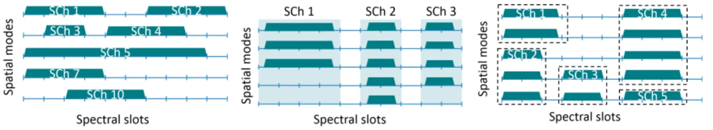
(a) SDM switching scheme 1 (b) SDM switching scheme 2 (c) SDM switching scheme 3 Figure 1: Illustration of forming superchannels in different SDM switching schemes.
a preliminary heuristic. This paper extends the work by (i) proposing mixed integer linear programming (MILP) formu-lations and refined heuristic algorithms for each of the SDM switching schemes in [20], and (ii) presenting simulation results based on new traffic profiles that follow the realistic flow size distribution [16]–[19].
The remainder of this paper is organized as follows. In Section II, the SDM switching schemes considered in this work are briefly introduced. The statement and objectives of the resource allocation problem are described in Section III. In Section IV, the MILPs and heuristics used to solve the problem are presented. Section V discusses numerical results. Concluding remarks are found in Section VI.
II. SDM SWITCHINGSCHEMES
As illustrated in Fig. 2, a simple modular DC network topology [6] is studied in this paper, where the PODs are interconnected through a single optical large port count (LPC) SDM switch. Each POD is connected to the LPC switch with a single bidirectional SDM fiber. In this paper, we analyze three different SDM switching schemes proposed in previous studies [5], [6] for modular DCs [4]. Each scheme provides a certain level of network flexibility by utilizing the spatial elements offered by the SDM fiber differently.
The first scheme (A1) is referred to asuncoupled SDM with flexible-grid WDM. This architecture requries one conventional spectrum selective switch (SSS) and one spatial mux/demux per spatial element for each transmission direction of the SDM fiber [21], [22]. Flexible-grid and tunable transceivers are deployed inside the PODs to transmit/receive spectral su-perchannels [6]. As shown in Fig. 1(a), each spatial element in A1 operates as an independent flexible-grid WDM fiber where multiple independent spectral superchannels are established.
Figure 2: The modular DC network topology.
The second scheme (A2) is thecoupled SDM with spectral flexibility, which is illustrated in Fig. 1(b). This architec-ture can be realized by equipping each POD with advance flexible-grid, tunable, MIMO transceivers to transmit/receive the spectral–spatial superchannels [22], [23]. Two large SSSs are employed to connect the PODs to the LPC switch [6]. In this scheme, spectral superchannels are expanded to all the spatial elements to create spectral–spatial superchannels with increased capacity.
The third scheme (A3) is the coupled SDM with spectral and spatial flexibility as displayed in Fig. 1(c), where the unrestricted flexibility in both spectral and spatial domains are exploited to form flexible spectral–spatial superchannels. In this architecture, the POD is also equipped with advance flexible-grid, tunable, MIMO transceivers to transmit/receive the spectral–spatial superchannels. In addition, it requires a large spectral and spatial selective switch (SSSS) to connect each POD to the SDM fiber [6].
Furthermore, assuming uncoupled spatial elements in SDM fibers, superchannels can use different spatial elements at the input and output fiber links to the switch [3], [4], [6]. However, the spectral continuity constraint is imposed on the superchannels to obtain transparent transmission.
III. PROBLEMSTATEMENT ANDOPTIMIZATION OBJECTIVES
To solve the resource allocation problem in SDM-based modular DCs, we assign spectral and spatial resources to a set of connection requests to connect the source and destination PODs. Based on the specific SDM switching scheme, different spectral–spatial superchannels can be established. In case the required resources are not available, the request is blocked.
In modular DCs, we consider that the network interconnect-ing PODs presents similar properties as the core tier of conven-tional DCs [6], whose traffic pattern varies slowly over time, on the order of several seconds or higher [16]–[18]. Hence, we assume in our offline traffic model that the connection requests in modular DCs change periodically at a fixed time interval. At the beginning of each time interval, taking the current estimation of the connection requests as an input, the resource allocation is performed offline and the corresponding network resources are reconfigured accordingly [5], [6].
The goal of the resource allocation problem is to optimize both the number of established connections C and the total throughput B in the modular DC network simultaneously.
The number of established connections C is related to the blocking probability κas C = (1−κ)|T|, where |T| is the number of connection requests. In our study, the two objectives are combined linearly as C+βB/tave, where β is a weight factor controlling the relative priority of B andC, while tave is a normalizing factor set equal to the average data rate. This objective has two components: the number of established connections is maximized when β = 0, while the throughput is optimized whenβ is large enough.
Assuming that the connection requests can be categorized intontraffic classes each with a data rateτifori∈ {1, . . . , n}, the objective proposed above can be rewritten as
n
X
i=1
(1 +βτi/tave)ci, (1) whereci is the number of established connections in class i. Equation (1) is a weighted sum of the numbers of established connections from different traffic classes in the network, where each traffic class is weighted by 1 +βτi/tave. By tuning the value of β, the relative importance of each traffic class in the objective function is varied accordingly. This interpretation is of practical relevance because not all the traffic in the DC is equally important [17], [18]. For example, the failure of deliv-ering short control messages may result in severe performance degradation, whereas a large volume data transfer usually has higher delay tolerance. Therefore, by differentiating the traffic classes, the resources in modular DC networks can be allocated more efficiently.
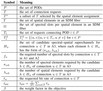
IV. RESOURCEALLOCATIONALGORITHMS In this section, we first present MILP formulations for the considered SDM switching schemes and then describe heuristic algorithms to provide close-to-optimal solutions to the resource allocation problems. The parameters and variables in the formulations are defined in Table I and II, respectively. The cardinal number of a set Ais denoted as|A|.
Table I: INPUT PARAMETERS Symbol Meaning
P the set of PODs
T the set of connection requests
Ts a subset ofT selected by the spatial element assignment
Γ the set of spatial elements in an SDM fiber
Ω the set of spectral slots per spatial element in an SDMfiber
Ti the set of requests connecting PODi∈P
T2
i Ti2={(u, v)|u, v∈Ti, u6=v}fori∈P
Hu
the set of candidate spectral–spatial superchannels for connectionu ∈T in A3, where each elementh ∈Hu
has the form of(κuh, λuh)
fu the required number of spectral slots by connectionin A1 and A2 u∈T
κuh the number of spectral elements required by the candidateh∈H uof connectionu∈T in A3
λuh the number of spatial elements required by the candidateh∈H uof connectionu∈T in A3
tu the requested bit rate of connectionu∈T
tave tave= |T1|Pu∈Ttu
β the weight factor in the objective
Table II: DECISION VARIABLES
Symbol Meaning
xiuk∈ {0,1}
equals 1 if the connectionu ∈ T in A1 uses the spatial elementk∈Γin the fiber connecting POD
i∈P
yu∈ {0,1} equals 1 ifu∈T is successfully provisioned
wu∈N+ the index of the first spectral slot assigned tou∈T δuv∈ {0,1}
equals 1 if the first spectral slot assigned to u is smaller than the first spectral slot assigned tovfor
(u, v)∈ ∪i∈PTi2
riu∈N+ the index of the first spatial element assigned toT u∈
iin A3,i∈P
zuh∈ {0,1} equals 1 ifu∈T in A3 selects candidateh∈Hu
γiuv∈ {0,1} equals 1 if(u, v)∈T2uandvin A3 share any spatial element,
i, i∈P
qiuv∈ {0,1}
equals 1 ifuandvin A3 do not share any spatial element and the indexes of all the spatial elements inuare smaller than those inv,(u, v)∈T2
i, i∈P
puv∈ {0,1} equals 0 if u and v in A3 are both successfully
established,(u, v)∈ ∪i∈PTi2
κu∈N+ the required number of spectral elements byin A3 u∈T
λu∈N+ the required number of spatial elements byin A3 u ∈T
A. Mixed Integer Linear Programming
The objective of all the formulations is the same as pre-sented in Section III. By writing the number of established connections and total throughput as C = P
u∈Tyu and
B=P
u∈Ttuyu, respectively, the objective can be expressed as P
u∈T(1 +βtu/tave)yu. All the formulations have sim-ilar constraints related to the formation of spectral–spatial superchannels, e.g., the spectral and spatial nonoverlapping constraints, but their implementations vary due to different levels of flexibilities.
1) A1: The MILP formulation for the resource allocation in A1 is presented in (2). Constraint (2b) calculates whether or not a connection request is successfully established. Constraint (2c) specifies the value of the first spectral slot’s index assigned to a connection request. Constraints (2d) and (2e) enforce spectral nonoverlapping by ensuring that each spectral slot on a certain link is allocated to at most one connection request. maximize yu,xiuk,wu,δuv P u∈T(1 +βtu/tave)yu (2a) subject to yu=Pk∈Γxiuk ∀u∈T, i∈u (2b) 1≤wu+fu−1≤ |Ω| ∀u∈T (2c) δuv+δvu= 1 ∀(u, v)∈T 2 i, i∈P (2d) wu+fu−wv+|Ω|(δuv+ xiuk+xivk)≤3|Ω| ∀(u, v)∈Ti2, i∈P, k∈Γ. (2e)
2) A2: The MILP for the resource allocation in A2 is modeled in (3). Constraint (3b) calculates whether or not a connection request is successfully established. It also imposes upper and lower bounds on the first spectral slot’s index of connection request u. Constraint (3c) specifies the spectral
order of two connection requests if they share a common SDM fiber. Constraint (3d) is the spectral nonoverlapping constraint.
maximize yu,wu,δuv P u∈T(1 +βtu/tave)yu (3a) subject to yu≤wu≤(|Ω| −fu+ 1)yu ∀u∈T (3b) δuv+δvu= 1 ∀(u, v)∈Ti2, i∈P (3c) wu+fu−wv+|Ω|(δuv+ yu+yv)≤3|Ω| ∀(u, v)∈T 2 i, i∈P. (3d)
3) A3: The MILP formulation for the resource allocation in A3 is formalized in (4). Since multiple spectral–spatial superchannels can be used to serve a single connection request, we use a precalculated set Hu to present all the candidates available to a connection requestu∈T. Each elementh∈Hu is characterized by a tuple (κuh, λuh), where κuh and λuh are the number of spectral and spatial elements needed by a superchannel h∈Hu, u∈T. maximize P u∈T(1 +βtu/tave)yu (4a) subject to wu+κu−1≤ |Ω| ∀u∈T (4b) riu+λu−1≤ |Γ| ∀u∈T, i∈u (4c) κu=Ph∈Huκuhzuh ∀u∈T (4d) λu=Ph∈Huλuhzuh ∀u∈T (4e) yu=Ph∈Huzuh ∀u∈T (4f) δuv+δvu= 1 ∀(u, v)∈Ti2, i∈P (4g) 1−puv≤yu 1−puv≤yv puv ≤2−yv−yu ∀(u, v)∈T2 i, i∈P (4h)
γiuv+qiuv+puv≤1 ∀(u, v)∈Ti2, i∈P (4i)
riu−(riv+λv−1) ≤ |Γ|(1−γiuv) ∀(u, v)∈T 2 i, i∈P (4j) riv−(riu+λu−1) ≤ |Γ|(1−γiuv) ∀(u, v)∈T 2 i, i∈P (4k) riu+λu−riv ≤ |Γ|(1−qiuv) ∀(u, v)∈T 2 i, i∈P (4l) riv+λv−riu ≤ |Γ|(qiuv+γiuv+puv) ∀(u, v)∈T 2 i, i∈P (4m) wu+κu−wv+|Ω|(δuv+ γiuv)≤2|Ω| ∀(u, v)∈T 2 i, i∈P. (4n)
Constraints (4b) and (4c) specify the first spectral and spatial element assigned to a connection request, respectively. Constraints (4d) and (4e) calculate the number of spectral and spatial element used by a connection request, respectively. Constraint (4f) calculates whether or not a connection request is successfully established. Constraint (4g) specifies the rela-tive spectral position of two connections if they share an SDM fiber. Constraint (4h) is equivalent to 1−puv =yuyv. Thus,
puv equals 0 if both uandv are successfully provisioned. In constraint (4i), given two established connections uandv on POD i (puv = 0), their relative position can only be one of
three cases: (i) uandv do not share any spatial element and all the spatial elements’ indices in u are less than those in
v (qiuv = 1 and γiuv = 0), (ii) uand v share some spatial element (qiuv= 0andγiuv = 1), and (iii)uandvdo not share any spatial element and all the spatial elements’ indices inu
are larger than those inv(qiuv = 0andγiuv= 0). Constraints (4j) and (4k) specify the relative spatial position ofuandvin case (i). Constraints (4l) and (4m) specify the relative spatial position of u and v in cases (ii) and (iii). Constraint (4n) specifies the relative spectral position ofuandvif they share any spatial element.
B. Heuristics
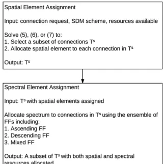
MILPs for resource allocation are too complex to be solved in realistic scale modular DCs2. This is due to the two-dimensional degrees of freedom for selecting resources. How-ever, as is shown by the algorithm outline in Fig. 3, we can leverage the MILP formulations to partly relieve their complexities by decomposing them into spatial and spectral assignment subproblems and solve them sequentially. First, we use the spatial element assignment (SEA) to generateTs, a subset of promising connection requests that are likely to be provisioned, and assign spatial elements to them. Then the spectral resources are assigned by solving an ensemble of first-fits (FFs) and choosing the best solution in the ensemble.
Specifically, the SEA MILPs can be formulated as follows for each scheme.
1) A1: maximize xiuk,yu P u∈T(1 +βtu/tave)yu (5a) subject to yu=Pk∈Γxiuk ∀u∈T, i∈u (5b) P u∈Tifuxiuk≤ |Ω| ∀i∈P, k∈Γ. (5c)
2On a 3.4 GHz quad-core computer with 8 GB RAM, the computational times of (2), (3), and (4) are approximately 1 hour, 30 minutes, and more than 24 hours, respectively.
Algorithm 1 The mixed FF algorithm Input:
• A set of connection requestsTsselected by the SEA • Normalized weight factors pi = Pn1+βτi/tave
i=11+βτi/tave for
each traffic classi= 1, . . . , n
1: Let D be an empty list 2: while Ts is not emptydo
3: Sample a traffic classiwith the probability equals to
pi for i= 1, . . . , n
4: Uniformly sample a connection request u from the traffic classi inTs
5: Appenduto the end ofD and delete it from Ts 6: end while
7: Allocate spectral resources to connections inLone by one Output: The spectrum assignments of established connec-tions, i.e., the value ofwufor all SDM switching schemes.
Figure 3: Outline of the proposed heuristic algorithm. 2) A2: maximize yu P u∈T(1 +βtu/tave)yu (6a) subject to P u∈Tifuyu≤ |Ω| ∀i∈P. (6b) 3) A3: maximize zuh,κu,yu P u∈T(1 +βtu/tave)yu (7a) subject to yu=Ph∈Huzuh ∀u∈T (7b) κu=Ph∈Huκuhzuh ∀u∈T (7c) P u∈Tiκu≤ |Ω| ∀i∈P. (7d)
As can be seen from (5)–(7), the SEA subproblem is mod-eled by dropping all constraints related to the relative spectral position of connections in (2)–(4) and adding a constraint imposing that the capacity of each spatial element is not exceeded by the sum of the connections’ capacities assigned to it. As a relaxed version of the original MILP, the SEA also calculates upper bounds of the objective functions for (2)– (4). Consequently, even when it is impossible to solve (2)–(4) exactly, we can obtain an estimation of the optimal solution without heavy computational burdens.
The set of promising connection requests delivered by the SEA, i.e., Ts={u|y
u = 1} in the solutions of (5)–(7), will enter the spectral element assignment stage, which is solved by an ensemble of FFs, and the final solution is the best one in the ensemble. Each of the FFs first sorts the connections according to a certain policy and then assigns spectral slots to each of them. Note that the spatial elements of each connection are already determined by the SEA and will not be changed later by the FFs.
In the ensemble of FFs, the connections are sorted by one of the following policies
i) ascending FF: ascending order of the bit rate request
tu, u∈T [24];
ii) descending FF: descending order of the bit rate request
tu, u∈T [25];
iii) mixed FF: a mixed order as described in Algorithm 1. Each traffic class appears in the top of the list with probabilities proportional to their relative priorities in the objective expressed in (1).
V. NUMERICALRESULTS
In this section, we first examine the performance of the proposed heuristics against the upper bounds on the objectives of the resource allocation problems given by the SEAs. We next study the relationship between the number of established connection requests and total throughput in the schemes in-troduced in Section II. The impact of the scheme and traffic load on the trade-off is also investigated. Finally, the trade-off is studied also under random traffic.
The dual-polarization binary phase-shift keying is assumed as the modulation format in the modular DC network. The spectrum is sliced into spectral slots of 12.5 GHz and the number of spectral slots is linearly mapped to the provisioned capacity. A guardband of one spectral slot is assigned to each spatial element of a spectral–spatial superchannel to guarantee a satisfactory signal quality. Due to the short transmission distance inside DCs and assigned guardband, the physical-layer impairments are negligible and not considered in this paper.
The number of connection requests generated per POD is a random integer uniformly distributed in the range
[L1(|P| −1), L2(|P| −1)], where|P|is the number of PODs in the modular DC and L1 and L2 with 0 < L1 < L2 <1 are two parameters controlling the range of the uniform distribution. Assuming that multiple flows between the same POD pair are consolidated into a single one [26], there is at most one connection request between two PODs. Two traffic classes are generated: τ1 = 50 Gbps mice flows and
τ2 = 400 Gbps elephant flows. The high data rate of mice flow is because we aggregate many mice flows between two PODs into one traffic request. Two types of traffic profiles with
L1= 0.10, L2= 0.95 andL1= 0.10, L2= 0.35are used in the simulations. The L1 = 0.10, L2 = 0.95 traffic profile is used for A1 and A3, while L1= 0.10, L2= 0.35is used for A2. This is because the resource utilization of A2 is much lower than those of A1 and A3 when a large amount of mice flows are present exhausting the spatial resources. Therefore, we need to adjust the traffic load for A2 to generate useful results. The value ofβ is gradually varied from 0 to 10. The elephant flows constitute10%of the total number of flows and produce42%of the aggregate data rate request, which follows the flow size distribution in empirical studies on DC traffic models [16]–[19]. A modular DC with|P|= 200,|Ω|= 80, and |Γ| = 5 is used in the simulations. The choice of these parameters can simplify the simulation process. Actually, the overall capacity offered by the SDM fiber is comparable
10−3 10−2 10−1 100 101 0% 10% 20% 30% 40% β Relativ e optimalit y gap 10−3 10−2 10−1 100 101 0% 5% 10% 15% 20% β 10−3 10−2 10−1 100 101 0% 20% 40% 60% 80% β
SEA+ensemble of FFs (proposed) Ascending FF Descending FF
A1 atL1= 0.10, L2= 0.95 A2 atL1= 0.10, L2= 0.35 A3 atL1= 0.10, L2= 0.95
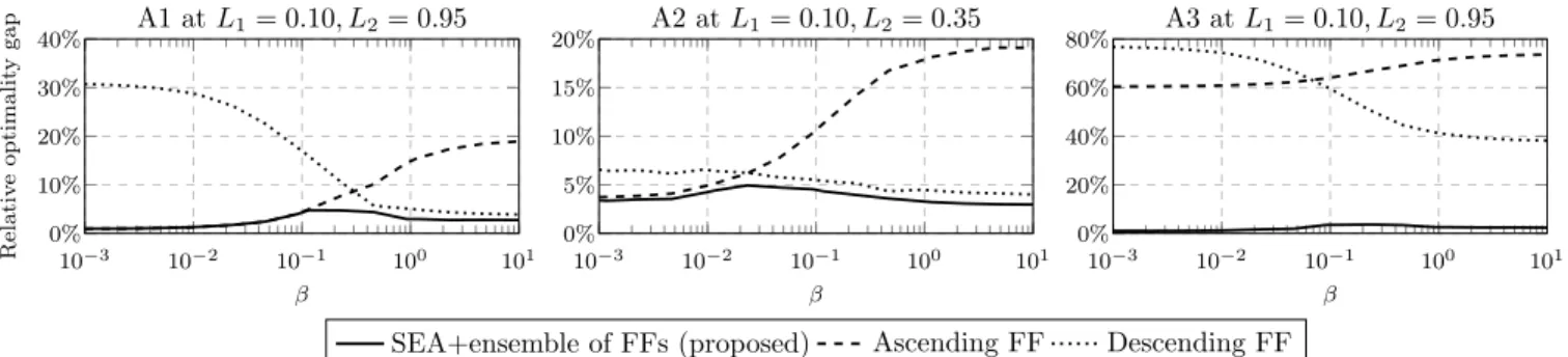
Figure 4: Relative optimality gaps against the upper bounds for all the schemes.
to a WDM system utilizing full C-band, but the cabling complexity and energy efficiency of the network is improved. Moreover, the proposed heuristic can easily scale up for larger DC networks with more spatial and spectral elements and obtain similar results since the complexity of the SEA and the ensemble of FFs are is affected by the network size. As will be shown, the trade-off between throughput and blocking probability depends only on the relative traffic load and is not related to the absolute DC size, so the selected parameters are sufficient to identify the general trade-offs in modular DCs.
A. Performance of Proposed Heuristic
The quality of the proposed heuristic algorithm can be measured by the relative optimality gap against the upper bound on the objective of the resource allocation calculated from the SEA, which is defined as
g= (ηub−ηhe)/ηub, (8) where ηub and ηhe are the values of the objectives given by the SEA and the ensemble of FFs, respectively. The optimal
solutions from the MILPs are not used in the calculation of the optimality gap because the computational complexities of MILPs are too high and cannot be solved within reasonable time. However, as will be shown below, the optimality gap is very close to zero, indicating tight upper and lower bounds estimated by the SEA and proposed heuristics, respectively.
In Fig. 4, the relative optimality gaps of the proposed heuristic are shown together with the benchmark ascending and descending FFs proposed in [6] for all the schemes. Note that the baseline FF algorithms in Fig. 4 are used for both the spatial and spectral assignments, and are different from the proposed heuristic, which assigns spatial resources by the SEA and spectral resources with the ensemble of FFs. Different traffic profiles are used for the schemes to make meaningful comparisons. As illustrated in Fig. 4, the relative optimality gaps of the proposed heuristic algorithms are close to 0 and outperform the FF benchmarks for all the schemes and all β, indicating good approximations of the optimal solutions in all cases. The gap of the benchmark ascending FF grows as β increases, since it prioritizes mice flows and, thus, performs well only whenβ is small. However, the opposite happens for the benchmark descending FF, which
3,700 4,100 4,500 4,900 300 320 340 360 β= 0.23 Established connections Throughput (Tbps) Upper bound Heuristic (a) A1 at L1= 0.10, L2= 0.95 1,200 1,400 1,600 1,800 2,000 100 150 200 250 Established connections Throughput (Tbps) Upper bound Heuristic (b) A2 atL1= 0.10, L2 = 0.95 3,600 4,000 4,400 4,800 300 320 340 360 β= 0.23 Established connections Throughput (Tbps) Upper bound Heuristic (c) A3 atL1= 0.10, L2= 0.95 1,000 2,000 3,000 4,000 5,000 150 250 350 Established connections Throughput (Tbps) (d) All schemes atL1= 0.10, L2= 0.95 1,500 1,600 1,700 1,800 1,900 100 120 140 160 β= 0.04 Established connections Throughput (Tbps) (e) A2 atL1= 0.10, L2= 0.35 1,600 1,800 2,000 2,200 100 150 200 Established connections Throughput (Tbps) (f) All schemes atL1= 0.10, L2= 0.35 Figure 5: Pareto curves for different schemes when |Γ|= 5,|Ω|= 80,|P|= 200. The traffic load isL1= 0.10, L2= 0.95in (a)–(d) and L1= 0.10, L2= 0.35 in (e) and (f).
allocates elephant flows first. In A1 and A2, the gains of the proposed algorithm against the benchmarks are comparatively large for medium values of β, when the mice and elephant flows are prioritized equally. In A3, thanks to the preselection of promising connection requests performed by the SEA, the proposed algorithm demonstrates a large performance improvement compared with the FF benchmarks. We also provide the solutions from the SEA and the ensemble of FFs to the MILP solver as start points to accelerate the search for better solutions. Unfortunately, no improvement is achieved within a reasonable time, due to the high complexity of the original MILPs.
B. Static Traffic Scenario
We then investigate the relation between the throughput and number of established connections. For each SDM switching scheme, we gradually change the value ofβ from 0 to 10 and solve the resource allocation problem 50 times with random traffic demands for each β. The throughput and established connections corresponding to the same β are averaged and plotted as one point in the throughput–connection plane. Finally, the points from different β values are connected to form a Pareto curve. The range of β is selected such that the throughput–connection trade-off is observable, whereas either the throughput or connection will be dominant when β is out of the chosen range.
In Fig. 5, the resulting Pareto curves for both the upper bounds on the objective of resource allocations obtained by the SEA and the proposed heuristic are shown for all the schemes. In Fig. 5(a) and 5(c), the Pareto curves of A1 and A3 bend towards the upper right corner of the throughput– connection plane. The “elbow points” correspond toβ = 0.23
in both schemes, which is highlighted by green ellipses. Asβ
increases from 0 to0.23, the upper bounds on the throughput increase by8%at the expense of3%less established connec-tions. If β increases above 0.23, the numbers of connections suffer more degeneration (15%in the upper bounds) whereas the improvement in throughput is not significant (only 6%in the upper bounds) compared to below the “elbow points”. The Pareto curves of the proposed heuristic follow a similar trend as the upper bounds. A balance between the throughput and the number of connections is achieved at the “elbow points”, where both objectives are optimized without affecting each
10−3 10−2 10−1 100 101 5% 10% 15% β P ercen tage of elephan t flo ws A1 A2 A3
Figure 6: The fraction of the number of elephant flows in the established connections for all the schemes.
0 125 250 375 500 625 0% 20% 40% 60% 80% 100% Data rate (Gbps) P ercen tage of CDF σ1=σ2= 0 Gbps σ1=σ2= 25 Gbps σ1=σ2= 50 Gbps σ1=σ2= 75 Gbps
Figure 7: The CDFs of the traffic models with the same average data rates (µ1 = 50, µ2 = 400 Gbps) but different standard deviations.
other significantly.
In Fig. 5(b), however, we can only observe two extremes on the Pareto curves in A2. The results stay at the bottom-right corner of the figure when β <0.5 and immediately jump to the upper left corner forβ >0.5. This is because A2 has much lower resource utilization compared with A1 and A3 and, thus, is over-loaded given the same connection requests as A1 and A3. Whenβ is small, the large number of mice flows exhaust all the resources and the elephant flows are entirely blocked. On the other hand, whenβis large enough, the elephant flows will suddenly take over and consume most of the resources, making the resource allocation problem hardly adjustable. The Pareto curve for A2 will be bent when the traffic load is light enough such that the resources are not fully dominated by only one traffic class but shared with multiple ones. This is verified by the simulation with L1 = 0.10, L2 = 0.35, as shown in Fig. 5(e), where the “elbow point” occurs atβ= 0.04.
The Pareto curves of all the schemes are compared in Fig. 5(d) and 5(f) for medium (L1 = 0.10, L2 = 0.95) and light (L1 = 0.10, L2 = 0.35) traffic loads, respectively. The performances of A1 and A3 are always better than A2 due to the extra flexibility provided by the SDM switching schemes. In Fig. 5(d), the Pareto curves of the upper bounds for A1 and A3 are very close to each other for all values of β, whereas A3 slightly outperforms A1 on the proposed heuristic’s Pareto curves. In Fig. 5(f), A1 and A3 can provision all the connection requests, regardless of the value of β. Consequently, their Pareto curves shrink to an identical point on the throughput–
0 125 250 375 500 0% 20% 40% 60% 80% 100% Data rate (Gbps) P ercen tage of CDF µ1= 50,µ2= 400 Gbps µ1= 75,µ2= 425 Gbps µ1= 100,µ2= 450 Gbps µ1= 125,µ2= 475 Gbps
Figure 8: The CDFs of the traffic models with the same standard deviations (σ1=σ2= 25Gbps) but different average data rates.
10−7 10−5 10−3 10−1 0.2 0.3 0.4 β Blo cking probabilit y 10−7 10−5 10−3 10−1 0.2 0.4 0.6 0.8 β Blo cking probabilit y 10−7 10−5 10−3 10−1 60 80 100 β Throughput (Tbps) 10−7 10−5 10−3 10−1 20 40 60 80 β Throughput (Tbps) 1,300 1,400 1,500 1,600 100 120 140 160 180 Established connections Throughput (Tbps) σ1=σ2= 0 Gbps σ1=σ2= 25 Gbps σ1=σ2= 50 Gbps σ1=σ2= 75 Gbps
(e) The Pareto curves (a) The blocking probabilities of mice flows (b) The blocking probabilities of elephant flows
(c) The throughput of mice flows (d) The throughput of elephant flows
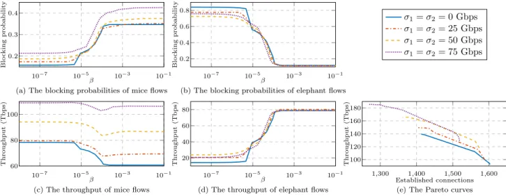
Figure 9: The simulation results for A2 with the traffic models shown in Fig. 7 (µ1= 50, µ2= 400Gbps).
connection plane. Moreover, analogous to the performance of A2 in the light traffic scenario, the Pareto curves of A1 and A3 will become straight lines under high traffic loads. These results show that the behavior of the Pareto curve is determined by the relative traffic load and is independent of the absolute DC size.
The fraction of the number of elephant flows in the estab-lished connections is a monotonically increasing function of
β for all the schemes as shown in Fig. 6, where the elephant flows grows near the “elbow points” and finally saturate at high β. The difference between the ending and beginning of the A2 curve is larger than in A1 and A3. This is because the flexibility of allocating spectral–spatial superchannels in A2 is less than those of A1 and A3, so only relatively coarse granular resource provisioning can be achieved in A2. As a result, compared with A1 and A3, more elephant flows are blocked in A2 when β is small, and more mice flows are blocked whenβ is large.
C. Stochastic Traffic Scenario
Next, we study the impact of stochastic traffic on the trade-off. Like in [27], we assume that the data rates of mice and elephant flows follow normal distributionsN(µ1, σ1)and
N(µ2, σ2), respectively, with negative values discarded and the distributions renormalized. Two simulation scenarios are considered. In the first scenario, the average data rates are fixed to µ1 = 50 and µ2 = 400 Gbps and the standard deviations of both flows are varied from 0 to 75 Gbps with a step size of 25 Gbps. The cumulative distribution functions (CDFs) of the chosen traffic models are shown in Fig. 7. In the second scenario, we simulate the traffic models with standard deviations fixed toσ1=σ2= 25Gbps and different average data rates. Hereµ1is swept from 50 to 125 Gbps andµ2from 400 to 475 Gbps, respectively, with a step size of 25 Gbps for both flows. The CDFs of the chosen traffic models are shown in Fig. 8.
In Fig. 9, the simulation results for A2 in the first traffic scenario are illustrated. Taking the case of σ1 = σ2 = 0 Gbps as a baseline, as the standard deviationsσ1andσ2grow, the blocking probabilities of mice flows increase in Fig. 9(a),
10−7 10−5 10−3 10−1 0 0.2 0.4 0.6 β Blo cking probabilit y 10−7 10−5 10−3 10−1 0 0.2 0.4 0.6 0.8 β Blo cking probabilit y 10−7 10−5 10−3 10−1 150 200 250 β Throughput (Tbps) 10−7 10−5 10−3 10−1 50 100 150 200 β Throughput (Tbps) 2,000 3,000 4,000 5,000 250 300 350 Established connections Throughput (Tbps) σ1=σ2= 0 Gbps σ1=σ2= 25 Gbps σ1=σ2= 50 Gbps σ1=σ2= 75 Gbps
(e) The Pareto curves (a) The blocking probabilities of mice flows (b) The blocking probabilities of elephant flows
(c) The throughput of mice flows (d) The throughput of elephant flows
10−7 10−5 10−3 10−1 0.2 0.3 0.4 0.5 β Blo cking probabilit y 10−7 10−5 10−3 10−1 0.2 0.4 0.6 0.8 β Blo cking probabilit y 10−7 10−5 10−3 10−1 100 150 β Throughput (Tbps) 10−7 10−5 10−3 10−1 20 40 60 80 100 β Throughput (Tbps) 1,200 1,300 1,400 1,500 1,600 100 150 200 Established connections Throughput (Tbps) µ1= 50,µ2= 400 Gbps µ1= 75,µ2= 425 Gbps µ1= 100,µ2= 450 Gbps µ1= 125,µ2= 475 Gbps
(e) The Pareto curves (a) The blocking probabilities of mice flows (b) The blocking probabilities of elephant flows
(c) The throughput of mice flows (d) The throughput of elephant flows
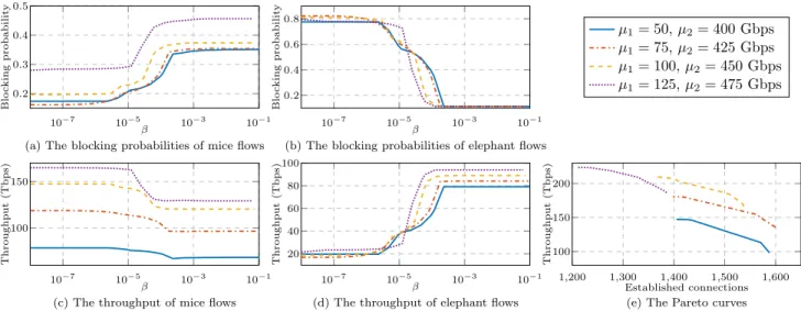
Figure 11: The simulation results for A2 with the traffic models shown in Fig. 8 (σ1=σ2= 25Gbps).
whereas those of elephant flows only fluctuate slightly in Fig. 9(b). In Fig. 9(c), the throughput of mice flows keeps increasing with an exception at σ1 =σ2 = 25 Gbps, where the throughput curve is initially very close to the baseline and has a slight increment only whenβis large. The throughput of elephant flows in Fig. 9(d) is almost unchanged relative to the baseline. In Fig. 9(e), the Pareto curves gradually move toward the upper left corner of the throughput–connection plane.
These observations are attributed to the large data rate granularity of superchannels in A2, truncated data rate dis-tribution of mice flows, and unbalanced number of mice and elephant flows. First, the smallest superchannel in A2 utilizes one spectral element and supports a maximum data rate of 125 Gbps, which is well above the average of mice flows. Additionally, as shown in Fig. 7, even at the highest data rate variation of 75 Gbps, still more than 70% of the mice flows can fit into the smallest superchannel. These mice flows do not consume extra resources but contribute more to the throughput since their data rate distribution is truncated from below and the probability mass is shifted to higher values.
On the other hand, as the data rate variation grows, the resource usage of connection requests becomes less uniform and, thus, causes heavier resource fragmentation and higher blocking probability. However, because the number of mice flows requiring the smallest superchannel are dominant over the remaining bigger mice flows and elephant flows, the overall throughput still grows despite the rising blocking probability. The exception in Fig. 9(c) is because the distribution of mice flows is not spread out enough to be truncated when
σ1=σ2= 25Gbps. Consequently, the throughput curve is the same as the baseline at smallerβ but gains a slight increment at larger β as the proposed heuristic prefers mice flows with larger data rate to optimize the overall objective.
In Fig. 10, the simulation results for A3 in the first traffic scenario are illustrated. Taking the case of σ1 = σ2 = 0 Gbps as a baseline, as the standard deviations σ1 and σ2 grow, the fragmentation becomes heavier and the blocking probabilities of both the mice and elephant flows in Fig. 10(a) and 10(b) increase. This is the reason why the Pareto curves in Fig. 10(e) are all shifted to the left and the throughput
10−7 10−5 10−3 10−1 0 0.2 0.4 0.6 0.8 β Blo cking probabilit y 10−7 10−5 10−3 10−1 0 0.2 0.4 0.6 0.8 1 β Blo cking probabilit y 10−7 10−5 10−3 10−1 150 200 250 300 350 β Throughput (Tbps) 10−7 10−5 10−3 10−1 0 100 200 β Throughput (Tbps) 2,000 3,000 4,000 250 300 350 400 Established connections Throughput (Tbps) µ1= 50,µ2= 400 Gbps µ1= 75,µ2= 425 Gbps µ1= 100,µ2= 450 Gbps µ1= 125,µ2= 475 Gbps
(e) The Pareto curves (a) The blocking probabilities of mice flows (b) The blocking probabilities of elephant flows
(c) The throughput of mice flows (d) The throughput of elephant flows
of the elephant flows in Fig. 10(d) drops. In Fig. 10(c), however, the throughput of mice flows behaves differently, where it first decreases at σ1 = 25 Gbps, then climbs up when σ1 = 50 Gbps, and finally becomes even higher than the baseline. When σ1 = 25 Gbps, the data rate distribution of mice flows is not spread out enough to be truncated, so the throughput of mice flows follows the reversed trend of its blocking probability. Whenσ1keeps growing, the distribution is truncated at zero and the average data rate of mice flow starts increasing. This effect cancels out with the reduced blocking probability at σ1 = 50 Gbps and becomes more significant when σ1 = 75 Gbps. Moreover, because of the dominant proportion of mice flows, the overall throughput follows the trend of mice flows and, thus, the Pareto curve first moves downward atσ1=σ2= 25Gbps and then upward.
The simulation results for A2 in the second traffic scenario are shown in Fig. 11. We consider the results ofµ1= 50, µ2=
400Gbps as a baseline. In Fig. 11(a), the blocking probability of mice flows stays the same atµ1= 75, µ2= 425Gbps, and then grows for larger average data rates. However, despite the fewer established mice flows, the throughput of mice flows keeps increasing in Fig. 11(c). This is because when the average data rates increases to µ1 = 75, µ2 = 425 Gbps, the mice flows can still fit into the smallest superchannel. Hence the mice blocking probability is the same but the mice throughput increases significantly. Larger average data rates will finally diversify the resource usage and cause heavier fragmentation and, thus, induce higher blocking probability to mice flows. Meanwhile, the mice throughput increases but at a lower growth rate due to the fewer number of established mice connections. In Fig. 11(b), the blocking probability of elephant flows stays close to the baseline curve with small fluctuations, whereas the throughput of elephant flows in Fig. 11(d) tends to follow the same behavior as the mice flows but in a much slighter degree. Combining the above mentioned effects together, the resulting Pareto curve in Fig. 11(e) first shifts upward at µ1 = 75, µ2 = 425 Gbps and then toward the upper left corner of the throughput–connection plane.
In Fig. 12, the simulation results for A3 in the second traffic scenario are illustrated. We consider the results of
µ1 = 50, µ2 = 400 Gbps as a baseline. As the average data rates grow, the blocking probability of mice flows in Fig. 12(a) increases as a result of heavier fragmentation. The throughput of mice flows in Fig. 12(c) also increases since the gain in average data rate outweighs the loss caused by higher blocking probability. In Fig. 12(b), the blocking probability of elephant flows grows at small β but converges to 0 when β is large. Consequently, the throughput of elephant flows in Fig. 12(d) decreases at small β, but the trend is reversed at largeβ. The resulting Pareto curve in Fig. 12(e) moves continuously toward the upper left corner of the throughput–connection plane.
The simulation results of A1 are very similar to those of A3 in both simulation scenarios and are shown in the paper. The only difference between them is that all Pareto curves of A1 are shifted slightly toward the lower left corner of the throughput–connection plane relative to their A3 counterparts. This is due to the limited switching flexibility offered by A1 in comparison with A3.
It is worth noting that the following figures of merit in DCNs are of great importance as well: i) bisection bandwidth, i.e., the minimum bandwidth available between any two equal segments of the DCN; ii) network latency, i.e., the time it takes for data to travel from its source to destination; and iii) scalability, i.e., the ability of the DCN to function well when it scales to a larger size. These key indicators are determined by both the resource allocation algorithm and DCN architecture. In this paper, due to the space limit, we mainly focus on the ef-ficiency of the resource allocation algorithm, whereas the other figures of merit are not thoroughly investigated. Qualitatively, an efficient and balanced algorithm can achieve a fair resource utilization in the DCN and, thus, obtains a relatively high bisection bandwidth. Moreover, the computational complexity of the proposed heuristic is relatively low and is not heavily dependent on the network size. Therefore, the network latency and scalability of the DCN can also benefit from the proposed algorithm. We plan to investigate this aspect in our future work.
VI. CONCLUSIONS
The paper presents both MILP formulations and heuristic algorithms for the resource allocation problem in three SDM-based modular DC switching schemes. The objective of the resource allocations is upper-bounded by the proposed SEA subproblem and tightly lower-bounded by the proposed heuris-tic algorithms. The trade-off between the number of estab-lished connections and throughput is identified. By plotting the interplay of the two objectives on the throughput–connection plane, we find that the best balance can be achieved at the “elbow point” of the Pareto curve, where both objectives are optimized simultaneously. Moreover, the shape of the Pareto curve is related to the relative traffic load and the SDM switching scheme. Despite A3’s extra flexibility, it has only slightly better performance compared with A1. Whereas A2 has the lowest achievable throughput and number of estab-lished connections due to the large resource granularity of its superchannels. The trade-off persists for all the architectures in random-traffic scenario, with shifts of the Pareto curves introduced by the specific traffic distributions and resource granularity.
ACKNOWLEDGMENT
Part of this paper was presented at the Optical Communica-tion Conference (OFC), Los Angeles, March 2017. This work was supported in part by the Swedish Research Council (VR) Grants 2012-5280 and 2014-6230.
REFERENCES
[1] J. Hamilton, “Architecture for modular data centers,” arXiv preprint cs/0612110, 2006.
[2] N. Farrington, G. Porter, S. Radhakrishnan, H. H. Bazzaz, V. Sub-ramanya, Y. Fainman, G. Papen, and A. Vahdat, “Helios: a hybrid electrical/optical switch architecture for modular data centers,” ACM Computer Communication Review, vol. 40, no. 4, pp. 339–350, 2010. [3] Y. Liu, H. Yuan, A. Peters, and G. Zervas, “Comparison of SDM and
WDM on direct and indirect optical data center networks,” in Proc. European Conference on Optical Communication (ECOC), D¨usseldorf, Germany, Sept. 2016, p. M.1.F.2.
[4] D. Klonidis, F. Cugini, O. Gerstel, M. Jinno, V. Lopez, E. Palkopoulou, M. Sekiya, D. Siracusa, G. Thou´enon, and C. Betoule, “Spectrally and spatially flexible optical network planning and operations,”IEEE Communications Magazine, vol. 53, no. 2, pp. 69–78, 2015.
[5] M. Fiorani, M. Tornatore, J. Chen, L. Wosinska, and B. Mukherjee, “Optical spatial division multiplexing for ultra-high-capacity modular data centers,” inProc. Optical Fiber Communication Conference (OFC), Anaheim, CA, Mar. 2016, pp. Tu2H–2.
[6] M. Fiorani, M. Tornatore, J. Chen, L. Wosinska, and B. Mukherjee, “Spatial division multiplexing for high capacity optical interconnects in modular data centers,” Journal of Optical Communications and Networking, vol. 9, no. 2, pp. 143–153, 2017.
[7] D. Siracusa, F. Pederzolli, P. Khodashenas, J. Rivas-Moscoso, D. Kloni-dis, E. Salvadori, and I. Tomkos, “Spectral vs. spatial super-channel allocation in SDM networks under independent and joint switching paradigms,” inProc. European Conference on Optical Communication (ECOC), Valencia, Spain, Sept. 2015, p. Mo.4.6.2.
[8] F. Pederzolli, D. Siracusa, J. M. Rivas-Moscoso, B. Shariati, E. Sal-vadori, and I. Tomkos, “Spatial group sharing for SDM optical networks with joint switching,” inProc. IEEE International Conference of Optical Network Design and Modeling (ONDM), Trento, Italy, May 2016, pp. 195–200.
[9] P. S. Khodashenas, J. M. Rivas-Moscoso, D. Siracusa, F. Pederzolli, B. Shariati, D. Klonidis, E. Salvadori, and I. Tomkos, “Comparison of spectral and spatial super-channel allocation schemes for SDM networks,”IEEE Journal of Lightwave Technology, vol. 34, no. 11, pp. 2710–2716, 2016.
[10] A. Muhammad, G. Zervas, D. Simeonidou, and R. Forchheimer, “Rout-ing, spectrum and core allocation in flexgrid SDM networks with multi-core fibers,” inProc. IEEE International Conference of Optical Network Design and Modeling (ONDM), Stockholm, Sweden, May 2014, pp. 192–197.
[11] D. J. Ives, P. Bayvel, and S. J. Savory, “Routing, modulation, spectrum and launch power assignment to maximize the traffic throughput of a nonlinear optical mesh network,” Photonic Network Communications, vol. 29, no. 3, pp. 244–256, 2015.
[12] D. J. Ives, P. Bayvel, and S. J. Savory, “Physical layer transmitter and routing optimization to maximize the traffic throughput of a nonlinear optical mesh network,” in Proc. IEEE International Conference of Optical Network Design and Modeling (ONDM), Stockholm, Sweden, May 2014, pp. 168–173.
[13] D. J. Ives, P. Bayvel, and S. J. Savory, “Adapting transmitter power and modulation format to improve optical network performance utilizing the Gaussian noise model of nonlinear impairments,”IEEE Journal of Lightwave Technology, vol. 32, no. 21, pp. 3485–3494, 2014. [14] S. Fujii, Y. Hirota, H. Tode, and K. Murakami, “On-demand spectrum
and core allocation for reducing crosstalk in multicore fibers in elastic optical networks,”Journal of Optical Communications and Networking, vol. 6, no. 12, pp. 1059–1071, 2014.
[15] M. N. Dharmaweera, L. Yan, M. Karlsson, and E. Agrell, “Nonlinear-impairments- and crosstalk-aware resource allocation schemes for multicore-fiber-based flexgrid networks,” inProc. European Conference on Optical Communication (ECOC), D¨usseldorf, Germany, Sept. 2016, p. Th2.P2.SC6.69.
[16] A. Greenberg, J. R. Hamilton, N. Jain, S. Kandula, C. Kim, P. Lahiri, D. A. Maltz, P. Patel, and S. Sengupta, “VL2: A scalable and flexible data center network,”ACM Computer Communication Review, vol. 39, no. 4, pp. 51–62, 2009.
[17] T. Benson, A. Anand, A. Akella, and M. Zhang, “Understanding data center traffic characteristics,”ACM Computer Communication Review, vol. 40, no. 1, pp. 65–72, 2010.
[18] T. Benson, A. Akella, and D. A. Maltz, “Network traffic characteristics of data centers in the wild,” inProc. Internet Measurement Conference, Melbourne, Australia, Nov. 2010, pp. 267–280.
[19] A. Roy, H. Zeng, J. Bagga, G. Porter, and A. C. Snoeren, “Inside the social network’s (datacenter) network,”ACM Computer Communication Review, vol. 45, no. 4, pp. 123–137, 2015.
[20] L. Yan, M. Fiorani, A. Muhammad, M. Tornatore, E. Agrell, and L. Wosinska, “Network performance trade-off in optical spatial divi-sion multiplexing data centers,” inProc. Optical Fiber Communication Conference (OFC), Los Angeles, CA, Mar. 2017, p. W3D.5. [21] B. Shariati, J.-M. Rivas-Moscoso, D. Marom, S. Ben-Ezra, D. Klonidis,
L. Velasco, and I. Tomkos, “Impact of spatial and spectral granularity on the performance of SDM networks based on spatial superchannel switching,”IEEE Journal of Lightwave Technology, vol. 35, no. 13, pp. 2559–2568, 2017.
[22] D. M. Marom, P. D. Colbourne, A. Derrico, N. K. Fontaine, Y. Ikuma, R. Proietti, L. Zong, J. M. Rivas-Moscoso, and I. Tomkos, “Survey of photonic switching architectures and technologies in support of spatially and spectrally flexible optical networking,”Journal of Optical Communications and Networking, vol. 9, no. 1, pp. 1–26, 2017. [23] D. M. Marom and M. Blau, “Switching solutions for WDM-SDM optical
networks,”IEEE Communications Magazine, vol. 53, no. 2, pp. 60–68, 2015.
[24] B. C. Chatterjee, N. Sarma, and E. Oki, “Routing and spectrum allocation in elastic optical networks: a tutorial,”IEEE Communications Surveys & Tutorials, vol. 17, no. 3, pp. 1776–1800, 2015.
[25] J. Zhao, H. Wymeersch, and E. Agrell, “Nonlinear impairment-aware static resource allocation in elastic optical networks,”IEEE Journal of Lightwave Technology, vol. 33, no. 22, pp. 4554–4564, 2015. [26] H. Rastegarfar, M. Glick, N. Viljoen, M. Yang, J. Wissinger, L.
La-Comb, and N. Peyghambarian, “TCP flow classification and bandwidth aggregation in optically interconnected data center networks,”Journal of Optical Communications and Networking, vol. 8, no. 10, pp. 777–786, 2016.
[27] B. Shariati, D. Klonidis, D. Siracusa, F. Pederzolli, J. Rivas-Moscoso, L. Velasco, and I. Tomkos, “Impact of traffic profile on the performance of spatial superchannel switching in SDM networks,” inProc. European Conference on Optical Communication (ECOC), Valencia, Spain, Sept. 2016, p. M.1.F.1.