Geometric deep learning:
going beyond Euclidean data
Michael M. Bronstein, Joan Bruna, Yann LeCun, Arthur Szlam, Pierre Vandergheynst
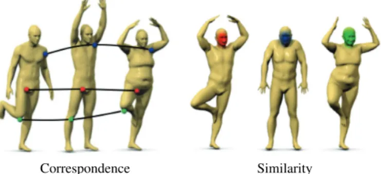
Many signal processing problems involve data whose un-derlying structure is non-Euclidean, but may be modeled as a manifold or (combinatorial) graph. For instance, in social networks, the characteristics of users can be modeled as signals on the vertices of the social graph [1]. Sensor net-works are graph models of distributed interconnected sensors, whose readings are modelled as time-dependent signals on the vertices. In genetics, gene expression data are modeled as signals defined on the regulatory network [2]. In neuro-science, graph models are used to represent anatomical and functional structures of the brain. In computer graphics and vision, 3D objects are modeled as Riemannian manifolds (surfaces) endowed with properties such as color texture. Even more complex examples include networks of operators, e.g., functional correspondences [3] or difference operators [4] in a collection of 3D shapes, or orientations of overlapping cameras in multi-view vision (“structure from motion”) problems [5].
The complexity of geometric data and the availability of very large datasets (in the case of social networks, on the scale of billions) suggest the use of machine learning techniques. In particular, deep learning has recently proven to be a powerful tool for problems with large datasets with underlying Euclidean structure.
The purpose of this paper is to overview the problems arising in relation to geometric deep learning and present solutions existing today for this class of problems, as well as key difficulties and future research directions.
I. INTRODUCTION
“Deep learning” refers to learning complicated concepts by building them from simpler ones in a hierarchical or multi-layer manner [6]. Artificial neural networks (ANNs) are popular realizations of such deep multi-layer hierarchies. In the past few years, the growing computational power of modern GPU-based computers and the availability of large training datasets have allowed successfully training ANNs with many layers and degrees of freedom [7]. This has led to qualitative breakthroughs on a wide variety of tasks, from speech recognition [8], [9] and machine translation [10] to image analysis and computer vision [11], [12], [13], [14], [15], [16], [17]. Nowadays, deep learning methods are widely used in commercial applications, including Siri speech recognition in Apple iPhone, Google text translation, and Mobileye vision-based technology for autonomously driving cars.
MB is with USI Lugano, Switzerland, Tel Aviv University, and Intel Perceptual Computing, Israel. JB is with Courant Institute, NYU and UC Berkeley, USA. YL with with Facebook AI Research and NYU, USA. AS is with Facebook AI Research, USA. PV is with EPFL, Switzerland.
Constructions that leverage the statistical properties of the data, in particular stationarity and compositionality through local statistics, which are present in natural images, video, and speech [18], [19], are one of the key reasons for the success of deep neural networks in these domains. These statistical properties have been related to physics [20] and formalized in specific classes of convolutional neural networks (CNNs) [21], [22], [23]. For example, one can think of images as functions on the Euclidean space (plane), sampled on a grid. In this setting, stationarity is owed to shift-invariance, locality is due to the local connectivity, and compositionality stems from the multi-resolution structure of the grid. These properties are exploited by convolutional architectures [24], which are built of alternating convolutional and downsampling (pooling) layers. The use of convolutions has a two-fold effect. First, it allows extracting local features that are shared across the image domain and greatly reduces the number of parameters in the network with respect to generic deep architectures (and thus also the risk of overfitting), without sacrificing the expressive capacity of the network. Second, as we will show in the following, the convolutional architecture itself imposes some priors about the data, which appear very suitable especially for natural images [25], [22].
While deep learning models have been particularly success-ful when dealing with signals such as speech, images, or video, in which there is an underlying Euclidean structure, recently there has been a growing interest in trying to apply learning on non-Euclidean geometric data, for example, in computer graphics and vision [26], [27], [28], natural language process-ing [29], and biology [30], [31]. The non-Euclidean nature of such data implies that there are no such familiar properties as global parameterization, common system of coordinates, vector space structure, or shift-invariance. Consequently, basic operations like linear combination or convolution that are taken for granted in the Euclidean case are even not well defined on non-Euclidean domains. This major obstacle that has so far precluded the use of successful deep learning meth-ods such as convolutional networks on generic non-Euclidean geometric data. As a result, the quantitative and qualitative breakthrough that deep learning methods have brought into speech recognition, natural language processing, and computer vision has not yet come to fields dealing with functions defined on more general geometric data.
II. GEOMETRIC LEARNING PROBLEMS
Broadly speaking, we can distinguish between two classes of geometric learning problems. In the first class of problems,
the goal is to characterize the structure of the data. For example, given a set of data points with some underlying lower dimensional structure embedded into a high-dimensional Euclidean space, we may want to recover that lower di-mensional structure. This is often referred to as manifold learning1 or non-linear dimensionality reduction, and is an
instance of unsupervised learning. Many methods for non-linear dimensionality reduction consist of two steps: first, they start with constructing a representation of local affinity of the data points (typically, a sparsely connected graph). Second, the data points are embedded into a low-dimensional space trying to preserve some criterion of the original affinity. For example, spectral embeddings tend to map points with many connections between them to nearby locations, and MDS-type methods try to preserve global information such as graph geodesic distances. Examples of such methods include differ-ent flavors of multidimensional scaling (MDS) [34], locally linear embedding (LLE) [35], stochastic neighbor embedding (t-SNE) [36], spectral embeddings such as Laplacian eigen-maps [37] and diffusion eigen-maps [38], and deep models [39]. Most recent approaches [40], [41], [42] tried to apply the successful word embedding model [43] to graphs. Instead of embedding the points, sometimes the graph can be processed directly, for example by decomposing it into small sub-graphs calledmotifs[44] orgraphlets[45].
In some cases, the data are presented as a manifold or graph at the outset, and the first step of constructing the affinity structure described above is unnecessary. For instance, in computer graphics and vision applications, one can analyze 3D shapes represented as meshes by constructing local geometric descriptors capturing e.g. curvature-like properties [46], [47]. In network analysis applications such as computational sociol-ogy, the topological structure of the social graph representing the social relations between people carries important insights allowing, for example, to classify the vertices and detect communities [48]. In natural language processing, words in a corpus can be represented by the co-occurrence graph, where two words are connected if they often appear near each other [49].
The second class of problems deals with analyzingfunctions
defined on a given non-Euclidean domain (these two classes are related, since understanding the properties of functions defined on a domain conveys certain information about the domain, and vice-versa, the structure of the domain imposes certain properties on the functions on it). We can further break down such problems into two subclasses: problems where the domain is fixed and those wheremultiple domains are given. Resorting again to the social network example, assume that we are given the geographic coordinates of users at different time, represented as a time-dependent signal on the vertices of the graph. An important application in location-based social networks is to predict the position of the user given his or her past behavior, as well as that of his or her friends [50]. In this problem, the domain (social graph) is assumed to be fixed; methods of signal processing on graphs, which have
1Note that the notion of “manifold” in this setting can be considerably more general than a classical smooth manifold; see e.g. [32], [33]
previously been reviewed in Signal Processing Magazine [51], can be applied to this setting, in particular, in order to define an operation similar to convolution in the spectral domain. This, in turn, allows generalizing CNN models to graphs [52], [53].
In computer graphics and vision applications, finding sim-ilarity and correspondence between shapes are examples of the second sub-class of problems: each shape is modeled as a manifold, and one has to work with multiple such domains. In this setting, a generalization of convolution in the spatial domain using local charting [54], [26], [28] appears to be more appropriate.
The main focus of this review is on this second class of problems, namely learning functions on non-Euclidean structured domains, and in particular, attempts to generalize the popular CNNs to such settings. We will start with an overview of Euclidean deep learning, summarizing the im-portant assumptions about the data, and how they are realized in convolutional network architectures. For a more in-depth review of CNNs and their and applications, we refer the reader to [7] and references therein.
Going to the non-Euclidean world, we will then define basic notions in differential geometry and graph theory. These topics are insufficiently known in the signal processing community, and to our knowledge, there is no introductory-level reference treating these so different structures in a common way. One of our goals in this review is to provide an accessible overview of these models resorting as much as possible to the intuition of traditional signal processing. We will emphasize the similari-ties and the differences between Euclidean and non-Euclidean domains, and distinguish between spatial- and spectral domain learning methods.
Finally, we will show examples of selected problem from the fields of network analysis, computer vision, and graph-ics, and outline current main challenges and potential future research directions.
III. DEEP LEARNING ONEUCLIDEAN DOMAINS
Geometric priors: Consider a compact d-dimensional Euclidean domain Ω = [0,1]d ⊂
Rd on which
square-integrable functions f ∈ L2(Ω) are defined (for example, in image analysis applications, images can be thought of as functions on the unit square Ω = [0,1]2). We consider a generic supervised learning setting, in which an unknown functiony: L2(Ω)→ Y is observed on a training set
{(fi∈L2(Ω), yi=y(fi))}i∈I. (1) In a supervised classification setting, the target space Y can be thought discrete with |Y|being the number of classes. In amultiple object recognitionsetting, we can replaceY by the
K-dimensional simplex, which represents the posterior class probabilitiesp(y|x). Inregressiontasks, we may considerY=
Rm.
In the vast majority of computer vision and speech analysis tasks, there are several crucial prior assumptions on the unknown function y. As we will see in the following, these assumptions are effectively exploited by convolutional neural network architectures.
Notation
Rm m-dimensional Euclidean space
a,a,A Scalar, vector, matrix
Ω, x Arbitrary domain, coordinate on it
f ∈L2(Ω) Square-integrable function on Ω
Tv Translation operator
τ,Lτ Deformation field, operator
ˆ
f Fourier transform off
f ? g Convolution off andg
X, TX, TxX Manifold, its tangent bundle, tangent space at x
h·,·,iTX Riemannian metric f ∈L2(X) Scalar field on manifoldX
F ∈L2(TX) Tangent vector field on manifold X ∇,div,∆ Gradient, divergence, Laplace operators V,E,F Vertices and edges of a graph,
faces of a mesh
f ∈L2(V) Functions on vertices of a graph
F ∈L2(E) Functions on edges of a graph
φi, λi Laplacian eigenfunctions, eigenvalues ht(·,·) Heat kernel
Φk Matrix of firstk Laplacian eigenvectors Λk Diagonal matrix of first kLaplacian
eigenvalues
ξ point-wise nonlinearity
wl,l0(x),Wl,l0 Convolutional filter in spatial and spectral domain
Stationarity:Atranslation operator2
Tvf(x) =f(x−v), x, v∈Ω, (2)
acts on functions f ∈ L2(Ω). Our first assumption is that the function y is either invariantor covariantwith respect to translations, depending on the task. In the former case, we have y(Tvf) =y(f) for anyf ∈ L2(Ω) andv ∈Ω. This is
typically the case in object classification tasks. In the latter, we havey(Tvf) =Tvy(f), which is well-defined when the output of the model is a space in which translations can act upon (for example, in problems of object localization, semantic segmentation, or motion estimation). Equivalently, we can describe this property in terms of the statistics of natural images. If one considers that natural images are drawn from an underlying probability distribution, the invariance/covariance property implies that this distribution describes a stationary source [18].
Local deformations and scale separation: Similarly, a de-formation Lτ, where τ : Ω → Ω is a smooth vector field,
acts on L2(Ω) as L
τf(x) =f(x−τ(x)). Deformations can
model local translations, changes in point of view, rotations and frequency transpositions [22].
Most tasks studied in computer vision are not only trans-lation invariant/covariant, but also stable with respect to local
2 We assume periodic boundary conditions to ensure that the operation is well-defined overL2(Ω).
deformations [55], [22]. In tasks that are translation invariant we have
|y(Lτf)−y(f)| ≈ k∇τk, (3)
for allf, τ. Here,k∇τk measures the smoothness of a given deformation field. In other words, the quantity to be predicted does not change much if the input image is slightly deformed. In tasks that are translation covariant, we have
|y(Lτf)− Lτy(f)| ≈ k∇τk. (4)
This property is much stronger than the previous one, since the space of local deformations has a high dimensionality, as opposed to thed-dimensional translation group.
It follows from (3) that we can extract sufficient statistics at a lower spatial resolution by downsampling demodulated localized filter responses without losing approximation power. An important consequence of this is that long-range depen-dencies can be broken into multi-scale local interaction terms, leading to hierarchical models in which spatial resolution is progressively reduced. To illustrate this principle, denote by
Y(x1, x2;v) = Prob(f(u) =x1 and f(u+v) =x2) (5) the joint distribution of two image pixels at an offsetv from each other. In the presence of long-range dependencies, this joint distribution will not be separable for any v. However, the deformation stability prior states that Y(x1, x2;v) ≈
Y(x1, x2;v(1 + )) for small . In other words, whereas long-range dependencies indeed exist in natural images and are critical to object recognition, they can be captured and down-sampled at different scales. This principle of stability to local deformations has been exploited in the computer vision community in models other than CNNs, for instance, deformable parts models [56].
In practice, the Euclidean domain Ω is discretized using a regular grid withn points; the translation and deformation operators are still well-defined so the above properties hold in the discrete setting.
Convolutional neural networks: Stationarity and sta-bility to local translations are both leveraged in convolutional neural networks (see insert IN1). A CNN consists of several
convolutional layersof the form g=CW(f), acting on a p
-dimensional input f(x) = (f1(x), . . . , fp(x)) by applying a
bank of filters W = (wl,l0), l = 1, . . . , q, l0 = 1, . . . , p and point-wise non-linearityξ, gl(x) = ξ p X l0=1 (fl0? wl,l0)(x) ! , (6)
and producing a q-dimensional output g(x) = (g1(x), . . . , gq(x)) often referred to as the feature maps.
Here,
(f ? w)(x) =
Z
Ω
f(x−x0)w(x0)dx0 (7) denotes the standard convolution. According to the local deformation prior, the filtersW have compact spatial support. Additionally, a downsampling or pooling layer g =P(f) may be used, defined as
[IN1] Convolutional neural networks: CNNs are currently among the most successful deep learning architectures in a variety of tasks, in particular, in computer vision. A typical CNN used in computer vision applications (see FIGS1) con-sists of multiple convolutional layers (6), passing the input image through a set of filtersW followed by point-wise non-linearityξ(typically, half-rectifiersξ(z) = max(0, z)are used, although practitioners have experimented with a diverse range of choices [6]). The model can also include a bias term, which is equivalent to adding a constant coordinate to the input. A network composed ofK convolutional layers put together
U(f) = (CW(K). . .◦CW(2)◦CW(1))(f)produces pixel-wise
features that are covariant w.r.t. translation and approximately covariant to local deformations. Typical computer vision
appli-cations requiring covariance are semantic image segmentation [14] or motion estimation [57].
In applications requiring invariance, such as image classifi-cation [13], the convolutional layers are typically interleaved with pooling layers (8) progressively reducing the resolution of the image passing through the network. Alternatively, one can integrate the convolution and downsampling in a single linear operator (convolution with stride). Recently, some au-thors have also experimented with convolutional layers which increase the spatial resolution using interpolation kernels [58]. These kernels can be learnt efficiently by mimicking the so-called algorithme `a trous [59], also referred to as dilated convolution.
Red Green Blue
Samoyed (16) ; ; ; Arctic fox (1.0); Eskimo dog (0.6); White wolf (0.4); Siberian husky (0.4)
Convolutions and ReLU Max pooling
Max pooling Convolutions and ReLU
Convolutions and ReLU Papillon (5.7) Pomeranzian (2.7)
[FIGS1]Typical convolutional neural network architecture used in computer vision applications (figure reproduced from [7]).
where N(x) ⊂ Ω is a neighborhood around x and G is a permutation-invariant function such as aLp-norm (in the latter case, the choice ofp= 1,2or∞results in average-, energy-, or max-pooling).
A convolutional network is constructed by composing sev-eral convolutional and optionally pooling layers, obtaining a generic hierarchical representation
UΘ(f) = (CW(K)· · ·P· · · ◦CW(2)◦CW(1))(f) (9)
where Θ = {W(1), . . . , W(K)} is the hyper-vector of the network parameters (all the filter coefficients). The model is said to be deep if it comprises multiple layers, though this notion is rather vague and one can find examples of CNNs with as few as a couple and as many as hundreds of layers [17]. The output features enjoy translation invariance/covariance depending on whether spatial resolution is progressively lost by means of pooling or kept fixed. Moreover, if one spec-ifies the convolutional tensors to be complex wavelet de-composition operators and uses complex modulus as
point-wise nonlinearities, one can provably obtain stability to local deformations [21]. Although this stability is not rigorously proved for generic compactly supported convolutional tensors, it underpins the empirical success of CNN architectures across a variety of computer vision applications [7].
In supervised learning tasks, one can obtain the CNN parameters by minimizing a task-specific costLon the training set{fi, yi}i∈I,
min
Θ
X
i∈I
L(UΘ(fi), yi). (10)
If the model is sufficiently complex and the training set is sufficiently representative, when applying the learned model to previously unseen data, one expects U(f) ≈ y(f). Al-though (10) is a non-convex optimization problem, stochastic optimization methods offer excellent empirical performance. Understanding the structure of the optimization problems (10) and finding efficient strategies for its solution is an active area of research in deep learning [60], [61], [62], [63].
A key advantage of CNNs explaining their success in numerous tasks is that the geometric priors on which CNNs are based result in a learning complexity that avoids the curse of dimensionality. Thanks to the stationarity and local deformation priors, the linear operators at each layer have a constant number of parameters, independent of the input size
n (number of pixels in an image). Moreover, thanks to the multiscale hierarchical property, the number of layers grows at a rate O(logn), resulting in a total learning complexity of O(logn)parameters.
IV. THE GEOMETRY OF MANIFOLDS AND GRAPHS
Our main goal is to generalize CNN-type constructions to non-Euclidean domains. In this paper, by non-Euclidean do-mains, we refer to two prototypical structures: manifolds and graphs. While arising in very different fields of mathematics (differential geometry and graph theory, respectively), in our context, these structures share several common characteristics that we will try to emphasize throughout our review.
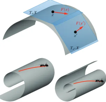
Manifolds: Roughly, a manifold is a space that is locally Euclidean. One of the simplest examples is a spherical surface modeling our Earth: around a point, it seems to be planar, which has led generations of people to believe in the flatness of the Earth. Formally speaking, a (differentiable)d-dimensional manifold X is a topological space where each point x has a neighborhood that is topologically equivalent (homeomorphic) to ad-dimensional Euclidean space, called the tangent space
and denoted by TxX (see Figure IV, top) The collection
of tangent spaces at all points (more formally, their disjoint union) is referred to as the tangent bundle and denoted by
TX. On each tangent space, we define an inner product h·,·iTxX :TxX ×TxX → R, which is additionally assumed to depend smoothly on the position x. This inner product is called a Riemannian metric in differential geometry and allows performing local measurements of angles, distances, and volumes. A manifold equipped with a metric is called
Riemannian manifold.
It is important to note that the definition of a Rieman-nian manifold is completely abstract and does not require a geometric realization in any space. However, a Riemannian manifold can be realized as a subset of a Euclidean space (in which case it is said to be embeddedin that space) by using the structure of the Euclidean space to induce a Riemannian metric. The celebrated Nash Embedding Theorem guarantees that any sufficiently smooth Riemannian manifold can be realized in a Euclidean space of sufficiently high dimension [64]. An embedding is not necessarily unique; two different realizations of a Riemannian metric are calledisometries.
Two-dimensional manifolds (surfaces) embedded into R3
are used in computer graphics and vision to describe boundary surfaces of 3D objects, colloquially referred to as ‘3D shapes’. This term is somewhat misleading since ‘3D’ here refers to the dimensionality of the embedding space rather than the manifold. Thinking of such a shape as made of infinitely thin material, inelastic deformations that do not stretch or tear it are isometric. Isometries do not affect the metric structure of the manifold and consequently, preserve any quantities that can be
TxX x F(x) Tx0X x0 F(x0)
Fig. 1. Top: tangent space and tangent vectors on a two-dimensional manifold (surface). Bottom: Examples of isometric deformations.
expressed in terms of the Riemannian metric (calledintrinsic). Conversely, properties related to the specific realization of the manifold in the Euclidean space are calledextrinsic.
As an intuitive illustration of this difference, imagine an insect that lives on a two-dimensional surface (Figure IV, bottom). The surface can be placed in the Euclidean space in any way, but as long as it is transformed isometrically, the insect would not notice any difference. The insect in fact does not even know of the existence of the embedding space, as its only world is 2D. This is an intrinsic viewpoint. A human observer, on the other hand, sees a surface in 3D space - this is an extrinsic point of view.
Calculus on manifolds: Our next step is to consider functions defined on manifolds. We are particularly interested in two types of functions: A scalar field is a smooth real functionf : X →R on the manifold. Atangent vector field F :X →TX is a mapping attaching a tangent vectorF(x)∈
TxX to each pointx. As we will see in the following, tangent
vector fields are used to formalize the notion of infinitesimal displacements on the manifold. We define the Hilbert spaces of scalar and vector fields on manifolds, denoted by L2(X) andL2(TX), respectively, with the following inner products:
hf, giL2(X) = Z X f(x)g(x)dx; (15) hF, GiL2(TX) = Z X hF(x), G(x)iTxXdx; (16)
dx denotes here ad-dimensional volume element induced by the Riemannian metric.
In calculus, the notion of derivative describes how the value of a function changes with an infinitesimal change of its argument. One of the big differences distinguishing classical calculus from differential geometry is a lack of vector space
j i wij Undirected graph j i k h αij βij ai aijk `ij Triangular mesh
[FIGS2] Two commonly used discretizations of a two-dimensional manifold: a graph and a triangular mesh.
[IN2] Laplacian on discrete manifolds: In computer graph-ics and vision applications, two-dimensional manifolds are commonly used to model 3D shapes. There are several com-mon ways of discretizing such manifolds. First, the manifold is assumed to be sampled at n points. Their embedding coordinatesx1, . . . ,xnare referred to aspoint cloud. Second, a graph is constructed upon these points, acting as its vertices. The edges of the graph represent the local connectivity of the manifold, telling whether two points belong to a neighborhood or not, e.g. with Gaussian edge weights
wij =e−kxi−xjk
2/2σ2
. (11)
This simplest discretization of the manifold, however, does not capture correctly the geometry of the underlying con-tinuous manifold (for example, the graph Laplacian would typically not converge to the continuous Laplacian operator of the manifold with the increase of the sampling density [65]). A geometrically consistent discretization is possible with an additional structure of faces F ∈ V × V × V, where (i, j, k) ∈ F implies (i, j),(i, k),(k, j) ∈ E. The collection of faces represents the underlying continuous manifold as a
polyhedral surface consisting of small triangles glued together. The triplet(V,E,F)is referred to astriangular mesh. To be a correct discretization of a manifold (amanifold mesh), every edge must be shared by exactly two triangular faces; if the manifold has a boundary, any boundary edge must belong to exactly one triangle.
On a triangular mesh, the simplest discretization of the Rie-mannian metric is given by assigning each edge a length
`ij>0, which must additionally satisfy the triangle inequality
in every triangular face. The mesh Laplacian is given by formula (25) with wij = −`2 ij+`2jk+` 2 ik 8aijk + −`2 ij+`2jh+` 2 ih 8aijh ; (12) ai = 13 X jk:(i,j,k)∈F aijk, (13) where aijk = p
sijk(sijk−`ij)(sijk−`jk)(sijk−`ik) is
the area of triangle ijk given by the Heron formula, and
sijk=12(`ij+`jk+`ki)is semi-perimeter of triangleijk. The
vertex weightaiis interpreted as the local area element (shown
in red in FIG2b). Note that the weights (12-13) are expressed solely in terms of the discrete metric`and thus intrinsic. When the mesh is infinitely refined under some technical conditions, such a construction can be shown to converge to the continuous Laplacian of the underlying manifold [66].
An embedding of the mesh (amounting to specifying the vertex coordinatesx1, . . . ,xn) induces a discrete metric`ij = kxi−xjk2, whereby (12) become thecotangent weights
wij =12(cotαij+ cotβij) (14) ubiquitously used in computer graphics [67].
structure on the manifold, prohibiting us from na¨ıvely using expressions likef(x+dx). The conceptual leap that is required to generalize such notions to manifolds is the need to work locally in the tangent space.
To this end, we define the differential of f as an op-erator df : TX → R acting on tangent vector fields. At
each point x, the differential can be identified with a linear form df(x) = h∇f(x), · iTxX acting on tangent vectors
F(x) ∈ TxX, which model a small displacement around x. The change of the function value as the result of this displacement is given by applying the form to the tangent vector, df(x)F(x) =h∇f(x), F(x)iTxX, and can be thought of as an extension of the notion of the classical directional derivative.
The operator ∇f : L2(X) → L2(TX) in the definition above is called the intrinsic gradient, and is similar to the classical notion of the gradient defining the direction of the steepest change of the function at a point, with the only differ-ence that the direction is now a tangent vector. Similarly, the
intrinsic divergence is an operator div : L2(TX) → L2(X) acting on tangent vector fields and (formal) adjoint to the
gradient operator [68],
hF,∇fiL2(TX)=h−divF, fiL2(X). (17)
Physically, a tangent vector field can be thought of as a flow of material on a manifold. The divergence measures the net flow of a field at a point, allowing to distinguish between field ‘sources’ and ‘sinks’. Finally, the Laplacian
(orLaplace-Beltrami operatorin differential geometric jargon) ∆ :L2(X)→L2(X)is an operator
∆f =−div(∇f) (18)
acting on scalar fields. Employing relation (17), it is easy to see that the Laplacian is self-adjoint (symmetric),
h∇f,∇fiL2(TX)=h∆f, fiL2(X)=hf,∆fiL2(X). (19)
The lhs in equation (19) is known as the Dirichlet energy in physics and measures the smoothness of a scalar field on the manifold (see insert IN3). The Laplacian can be interpreted as the difference between the average of a function on an infinitesimal sphere around a point and the value of the
function at the point itself. It is one of the most important oper-ators in mathematical physics, used to describe phenomena as diverse as heat diffusion (see insert IN4), quantum mechanics, and wave propagation. As we will see in the following, the Laplacian plays a center role in signal processing and learning on non-Euclidean domains, as its eigenfunctions generalize the classical Fourier bases, allowing to perform spectral analysis on manifolds and graphs.
It is important to note that all the above definitions are
coordinate free. By defining a basis in the tangent space, it is possible to express tangent vectors as d-dimensional vectors and the Riemannian metric as a d×d symmetric positive-definite matrix.
Graphs and discrete differential operators: Another type of constructions we are interested in are graphs, which are popular models of networks, interactions, and similarities between different objects. For simplicity, we will consider
weighted undirected graphs, formally defined as a pair(V,E), whereV={1, . . . , n}is the set ofnvertices, andE ⊆ V × V is the set of edges, where the graph being undirected implies that (i, j) ∈ E iff (j, i) ∈ E. Furthermore, we associate a weightai >0 with each vertexi∈ V, and a weightwij ≥0
with each edge(i, j)∈ E.
Real functions f : V → R and F : E → R on the
vertices and edges of the graph, respectively, are roughly the discrete analogy of continuous scalar and tangent vector fields in differential geometry.3 We can define Hilbert spacesL2(V) andL2(E)of such functions by specifying the respective inner products, hf, giL2(V) = X i∈V aifigi; (20) hF, GiL2(E) = X i∈E
wijFijGij. (21) Let f ∈ L2(V) and F ∈ L2(E) be functions on the vertices and edges of the graphs, respectively. We can define differential operators acting on such functions analogously to differential operators on manifolds [69]. The graph gradient
is an operator∇:L2(V)→L2(E)mapping functions defined on vertices to functions defined on edges,
(∇f)ij = fi−fj, (22)
automatically satisfying(∇f)ij =−(∇f)ji. Thegraph diver-genceis an operatordiv :L2(E)→L2(V)doing the converse,
(divF)i = 1 ai X j:(i,j)∈E wijFij. (23)
It is easy to verify that the two operators are adjoint w.r.t. the inner products (20–21),
hF,∇fiL2(E)=h∇∗F, fiL2(V)=h−divF, fiL2(V). (24)
The graph Laplacian is an operator ∆ : L2(V) →L2(V) defined as∆ =−div∇. Combining definitions (22-23), it can be expressed in the familiar form
(∆f)i = 1 ai X (i,j)∈E wij(fi−fj). (25)
3It is tacitly assumed here thatF isalternating, i.e.,F
ij=−Fji.
Note that formula (25) captures the intuitive geometric inter-pretation of the Laplacian as the difference between the local average of a function around a point and the value of the function at the point itself.
Denoting by W = (wij) the n × n matrix of edge weights (it is assumed that wij = 0 if (i, j) ∈ E/ ), by
A= diag(a1, . . . , an) the diagonal matrix of vertex weights, and by D = diag(P
j6=iwij) the degree matrix, the graph
Laplacian application to a functionf ∈L2(V)represented as a column vector f = (f1, . . . , fn)> can be written in matrix-vector form as
∆f = A−1(D−W)f. (26) The choice ofA=Iin (26) is referred to as theunnormalized graph Laplacian; another popular choice isA=Dproducing therandom walk Laplacian[70].
Discrete manifolds: As we mentioned, there are many practical situations in which one is given a sampling of points arising from a manifold but not the manifold itself. In computer graphics applications, reconstructing a correct discretization of a manifold from a point cloud is a difficult problem of its own, referred to a meshing (see insert IN2). In manifold learning problems, the manifold is typically ap-proximated as a graph capturing the local affinity structure. We warn the reader that the term “manifold” as used in the context of generic data science is not geometrically rigorous, and can have less structure than a classical smooth manifold. For example, a set of points that “looks locally Euclidean” in practice may have self intersections, infinite curvature, different dimensions depending on the scale and location at which one looks, extreme variations in density, and “noise” with confounding structure.
Fourier analysis on non-Euclidean domains: The Laplacian operator is a self-adjoint positive-semidefinite oper-ator, admitting on a compact domain4 an eigendecomposition
with a discrete set of orthonormal eigenfunctions φ0, φ1, . . . (satisfying hφi, φji=δij) and non-negative real eigenvalues 0 = λ0 ≤ λ1 ≤ . . . (referred to as the spectrum of the Laplacian),
∆φi=λiφi, i= 0,1, . . . (31) The eigenfunctions are the smoothest functions in the sense of the Dirichlet energy (see insert IN3) and can be interpreted as a generalization of the standard Fourier basis (given, in fact, by the eigenfunctions of the 1D Euclidean Laplacian, −d2
x2e
iωx=ω2eiωx) to a non-Euclidean domain. It is
impor-tant to emphasize that the Laplacian eigenbasis is intrinsic due to the intrinsic construction of the Laplacian itself.
A smooth square-integrable function f on the domain can be decomposed intoFourier seriesas
f(x) = X i≥0 hf, φiiL2(X) | {z } ˆ fi φi(x), (32)
4In the Euclidean case, the Fourier transform of a function defined on a finite interval (which is a compact set) or its periodic extension is discrete. In practical settings, all domains we are dealing with are compact.
[IN3] Physical interpretation of Laplacian eigenfunctions: Given a functionf on the domain X, theDirichlet energy
EDir(f) = Z X k∇f(x)k2dx= Z X f(x)∆f(x)dx,(27)
measures how smooth it is (the last identity in (27) stems from (19)). We are looking for an orthonormal basis on X, containing k smoothest possible functions, by solving the optimization problem min φ0 EDir(φ0) s.t. kφ0k= 1 (28) min φi EDir(φi) s.t. kφik= 1, i= 1,2, . . . k−1 φi⊥span{φ0, . . . , φi−1}. In the discrete setting, when the domain is sampled atnpoints, problem (28) can be rewritten as
min
Φk∈Rn×k
trace(Φ>k∆Φk) s.t. Φ>kΦk=I, (29)
whereΦk= (φ0, . . .φk−1). The solution of (29) is given by the firstkeigenvectors of ∆satisfying
∆Φk =ΦkΛk, (30) where Λk = diag(λ0, . . . , λk−1) is the diagonal matrix of corresponding eigenvalues. The eigenvalues0 =λ0 ≤ λ1 ≤
. . . λk−1 are non-negative due to positive-semidefiniteness of the Laplacian and can be interpreted as ‘frequencies’, where
φ0 = const with the corresponding eigenvalue λ0 = 0play the role of the DC.
The Laplacian eigendecomposition can be carried out in two ways. First, equation (30) can be rewritten as a gen-eralized eigenproblem (D − W)Φk = AΦkΛk, result-ing in A-orthogonal eigenvectors, Φ>kAΦk = I.
Alterna-tively, introducing a change of variables Ψk = A1/2Φk, we can obtain a standard eigendecomposition problem
A−1/2(D−W)A−1/2Ψ
k = ΨkΛk with orthogonal
eigen-vectors Ψ>kΨk = I. When A = D is used, the matrix
˜
∆=A−1/2(D−W)A−1/2 is referred to as thenormalized
symmetric Laplacian. 0 10 20 30 40 50 60 70 80 90 100 −0.2 0 0.2 0 max min Euclidean Manifold φ0 φ1 φ2 φ3 φ0 φ1 φ2 φ3 0 max min Graph φ0 φ1 φ2 φ3
[FIGS3]Example of the first four Laplacian eigenfunctionsφ0, . . . , φ3on a Euclidean domain (1D line, top left) and non-Euclidean domains
(human shape modeled as a 2D manifold, top right; and Minnesota road graph, bottom) domains. In the Euclidean case, the result is the
standard Fourier basis comprising sinusoids of increasing frequency. In all cases, the eigenfunctionφ0 corresponding to zero eigenvalue is
constant (‘DC’).
where the projection on the basis functions producing a discrete set of Fourier coefficients generalizes the analysis
(forward transform) stage in classical signal processing, and summing up the basis functions with these coefficients is the
synthesis (inverse transform) stage.
A centerpiece of classical Euclidean signal processing is the property of the Fourier transform diagonalizing the con-volution operator, colloquially referred to as the Convolution Theorem, allowing to express the convolution f ? g of two
functions in the spectral domain as the element-wise product of their Fourier transforms,
(f ? g[)(ω) = Z ∞ −∞ f(x)e−iωxdx Z ∞ −∞ g(x)e−iωxdx.(33)
Unfortunately, in the non-Euclidean case we cannot even define the operation x−x0 on the manifold or graph, so the notion of convolution does not directly extend to this case. One possibility to generalize convolution to non-Euclidean domains
is by using the convolution theorem as a definition, (f ? g)(x) = X
i≥0
hf, φiiL2(X)hg, φiiL2(X)φi(x). (34)
One of the key differences of such a construction from the classical convolution is the lack of shift-invariance. In terms of signal processing, it can be interpreted as a position-dependent filter. While parametrized by a fixed number of coefficients in the frequency domain, the spatial representation of the filter can vary dramatically at different points.
The discussion above also applies to graphs instead of manifolds, where one only has to replace the inner product in equations (32, 34) with the discrete one (20). All the sums over i would become finite, as the graph Laplacian ∆
hasn eigenvectors. In matrix-vector notation, the generalized convolutionf ? g can be expressed asGf =Φdiag(ˆg)Φ>f, where gˆ = (ˆg1, . . . ,ˆgn) is the spectral representation of the filter andΦdenotes the Laplacian eigenvectors (30). The lack of shift invariance results in the absence of circulant (Toeplitz) structure in the matrix G, which characterizes the Euclidean setting. Furthermore, it is easy to see that the convolution operation commutes with the Laplacian, G∆f =∆Gf.
Uniqueness and stability: Finally, it is important to note that the Laplacian eigenfunctions are not uniquely defined. To start with, they are defined up to sign (i.e.,∆(±φ) =λ(±φ)). Thus, even isometric domains might have different Laplacian eigenfunctions. Furthermore, if a Laplacian eigenvalue has multiplicity, then the associated eigenfunctions can be de-fined as orthonormal basis spanning the corresponding eigen-subspace (or said differently, the eigenfunctions are defined up to an orthogonal transformation in the eigen-subspace). A small perturbation of the domain can lead to very large changes in the Laplacian eigenvectors, especially those asso-ciated with high frequencies. At the same time, the definition of heat kernels (36) and diffusion distances (38) does not suffer from these ambiguities – for example, the sign ambiguity disappears as the eigenfunctions are squared. Heat kernels also appear to be robust to domain perturbations.
V. FREQUENCY-DOMAIN LEARNING METHODS
We have now finally got to our main goal, namely, con-structing a generalization of the CNN architecture on non-Euclidean domains. We will start with the assumption that the domain on which we are working is fixed, and for the rest of this section will use the problem of classification of a signal on a graph as the prototypical application.
Spectral CNN: We have seen that convolutions are linear operators that commute with the Laplacian operator. Therefore, given a weighted graph, a first route to generalize a convolutional architecture is by first restricting our interest on linear operators that commute with the graph Laplacian [71]. This property, in turn, implies operating on the spectrum of the graph weights, given by the eigenvectors of the graph Laplacian.
Similarly to the convolutional layer (6) of a classical Eu-clidean CNN, we define a spectral convolutional layeras
gl=ξ q X l0=1 ΦkWl,l0Φ>kfl0 ! , (39)
where the n×p and n×q matrices F = (f1, . . . ,fp) and G = (g1, . . . ,gq) represent the p- and q-dimensional input
and output signals on the vertices of the graph, respectively (we use n = |V| to denote the number of vertices in the graph),Wl,l0 is ak×kdiagonal matrix of spectral multipliers representing a filter in the frequency domain, and ξ is a nonlinearity applied on the vertex-wise function values. Using only the first k eigenvectors in (39) sets a cutoff frequency which depends on the intrinsic regularity of the graph and also the sample size. Typically, k n, since only the first Laplacian eigenvectors describing the smooth structure of the graph are useful in practice.
If the graph has an underlying group invariance, such a construction can discover it. In particular, standard CNNs can be redefined from the spectral domain (see insert IN5). However, in many cases the graph does not have a group structure, or the group structure does not commute with the Laplacian, and so we cannot think of each filter as passing a template acrossVand recording the correlation of the template with that location.
We should stress that a fundamental limitation of the spectral construction is its limitation to a single domain. The reason is that spectral filter coefficients (39) are basis dependent. It implies that if we learn a filter w.r.t. basis Φk
on one domain, and then try to apply it on another domain with another basisΨk, the result could be very different (see Figure V). It is possible to construct compatible orthogonal bases across different domains resorting to a joint diagonal-ization procedure [72], [73]. However, such a construction requires the knowledge of some correspondence between the domains. In applications such as social network analysis, for example, where dealing with two time instances of a social graph in which new vertices and edges have been added, such a correspondence can be easily computed and is therefore a reasonable assumption. Conversely, in computer graphics applications, finding correspondence between shapes is in itself a very hard problem, so assuming known correspondence between the domains is a rather unreasonable assumption.
Assuming that k = O(n) eigenvectors of the Laplacian are kept, a convolutional layer (39) requires pqk = O(n) parameters to train. We will see next how the global and local regularity of the graph can be combined to produce layers with constant number of parameters, i.e., such that the number of learnable parameters per layer does not depend upon the size of the input.
The non-Euclidean analogy of pooling isgraph coarsening, in which only a fraction α < 1 of the graph vertices is retained. The eigenvectors of graph Laplacians at two different resolutions are related by the following multigrid property: Let Φ, Φ¯ denote the n × n and αn × αn matrices of Laplacian eigenvectors of the original and the coarsened graph, respectively. Then, ¯ Φ≈PΦ Iαn 0 , (40)
where P is aαn×n binary matrix whoseith row encodes the position of the ith vertex of the coarse graph on the original graph. It follows that strided convolutions can be
[IN4] Heat diffusion on non-Euclidean domains: An im-portant application of spectral analysis, and historically, the main motivation for its development by Fourier, is the solution of partial differential equations (PDEs). In particular, we are interested in heat propagation on non-Euclidean domains. This process is governed by the heat diffusion equation, which in the simplest setting of homogeneous and isotropic diffusion has the form
(
ft(x, t) =−c∆f(x, t)
f(x,0) =f0(x) (Initial condition)
(35) with additional boundary conditions if the domain has a boundary. f(x, t) represents the temperature at point x at time t. Equation (35) encodes the Newton’s law of cooling, according to which the rate of temperature change of a body (lhs) is proportional to the difference between its own temperature and that of the surrounding (rhs). The proportion coefficientc is referred to as thethermal diffusivity constant. The solution of (35) is given by applying the heat operator Ht =e−t∆ to the initial condition and can be expressed in the spectral domain as
f(x, t) = e−t∆f0(x) = X i≥0 hf0, φiiL2(X)e−tλiφi(x)(36) = Z X f0(x0) X i≥0 e−tλiφi(x)φi(x0) | {z } ht(x,x0) dx0.
ht(x, x0) is known as the heat kernel and represents the solution of the heat equation with an initial conditionf0(x) =
δx0(x), or, in signal processing terms, an ‘impulse response’. In physical terms, ht(x, x0) describes how much heat flows from a point xto point x0 in time t. In the Euclidean case, the heat kernel is shift-invariant, ht(x, x0) = ht(x−x0),
allowing to interpret the integral in (36) as a convolution
f(x, t) = (f0?ht)(x). In the spectral domain, convolution with
the heat kernel amounts to low-pass filtering (with frequency response e−tλ). Larger values of diffusion time t result in
lower effective cutoff frequency and thus smoother solutions in space (corresponding to the intuition that longer diffusion smoothes more the initial heat distribution).
The ‘cross-talk’ between two heat kernels positioned at points
xandx0 allows to measure an intrinsic distance
d2t(x, x0) = Z X (ht(x, y)−ht(x0, y))2dy (37) = X i≥0 e−2tλi(φi(x)−φi(x0))2 (38)
referred to as thediffusion distance [38]. Note that interpret-ing (37) and (38) as spatial- and frequency-domain norms k · kL2(X) and k · k`2, respectively, their equivalence is the
consequence of theParseval identity. Unlikegeodesic distance
that measures the length of the shortest path on the manifold or graph, the diffusion distance has an effect of averaging over different paths. It is thus more robust to perturbations of the domain, for example, introduction or removal of edges in a graph, or ‘cuts’ on a manifold.
max
0
[FIGS4]Examples of heat kernels on non-Euclidean domains (man-ifold, top; and graph, bottom). Observe how moving the heat kernel to a different location changes its shape, which is an indication of the lack of shift-invariance.
generalized using the spectral construction by keeping only the low-frequency components of the spectrum. This property also allows us to interpret (via interpolation) the local filters at deeper layers in the spatial construction to be low frequency. However, since in (39) the non-linearity is applied in the spatial domain, in practice one has to recompute the graph Laplacian eigenvectors at each resolution and apply them directly after each pooling step.
The spectral construction (39) assigns a degree of free-dom for each eigenvector of the graph Laplacian. In most graphs, individual high-frequency eigenvectors become highly unstable. However, similarly as the wavelet construction in
Euclidean domains, by appropriately grouping high frequency eigenvectors in each octave one can recover meaningful and stable information. As we shall see next, this principle also entails better learning complexity.
Learning with smooth spectral multipliers: In order to achieve a good generalization, it is important to adapt the learning complexity to reduce the number of free parameters of the model. On Euclidean domains, this is achieved by learning convolutional kernels with small spatial support, which enables the model to learn a number of parameters independent of the input size. In order to achieve a similar learning complexity in the spectral domain, it is thus necessary to restrict the class of
[IN5] Rediscovering standard CNNs using correlation kernels: In situations where the graph is constructed from the data, a straightforward choice of the edge weights (11) of the graph is the covariance of the data. LetFdenote the input data distribution and
Σ=E(F−EF)(F−EF)> (41)
the data covariance matrix. If each point has the same variance
σii = σ2, then diagonal operators on the Laplacian simply
scale the principal components ofF.
In natural images, since their distribution is approximately stationary, the covariance matrix has a circulant structure
σij≈σi−j and is thus diagonalized by the standard Discrete
Cosine Transform (DCT) basis. It follows that the principal components ofFroughly correspond to the DCT basis vectors organized by frequency. Moreover, natural images exhibit a power spectrum E(|fb(ω)|2) ∼ |ω|−2, since nearby pixels
are more correlated than far away pixels [18]. It results that principal components of the covariance are essentially ordered from low to high frequencies, which is consistent with the standard group structure of the Fourier basis. When applied to natural images represented as graphs with weights defined by the covariance, the spectral CNN construction recovers the standard CNN, without any prior knowledge [74]. Indeed, the linear operators ΦWl,l0ΦT in (39) are by the previous
argument diagonal in the Fourier basis, hence translation invariant, hence classical convolutions. Furthermore, Section VII explains how spatial subsampling can also be obtained via dropping the last part of the spectrum of the Laplacian, leading to pooling, and ultimately to standard CNNs.
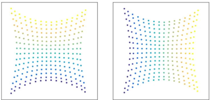
[FIG5a] Two-dimensional embedding of pixels in 16×16 image patches using a Euclidean RBF kernel. The RBF kernel is constructed
as in (11), by using the covarianceσijas Euclidean distance between
two features. The pixels are embedded in a 2D space using the first two eigenvectors of the resulting graph Laplacian. The colors in the left and right figure represent the horizontal and vertical coordinates of the pixels, respectively. The spatial arrangement of pixels is roughly recovered from correlation measurements.
Domain Basis Signal X Φ f X Φ ΦWΦ>f Y Ψ ΨWΨ>f
Fig. 2. A toy example illustrating the difficulty of generalizing spectral filtering across non-Euclidean domains. Left: a function defined on a manifold (function values are represented by color); middle: result of the application of an edge-detection filter in the frequency domain; right: the same filter applied on the same function but on a different (nearly-isometric) domain produces a completely different result. The reason for this behavior is that the Fourier basis is domain-dependent, and the filter coefficients learnt on one domain cannot be applied to another one in a straightforward manner.
spectral multipliers to those corresponding to localized filters. For that purpose, we have to express spatial localization of filters in the frequency domain. In the Euclidean case, smoothness in the frequency domain corresponds to spatial
decay, since Z |x|2k|f(x)|2dx=Z ∂kfˆ(ω) ∂ωk 2 dω , (42)
from the Parseval Identity. This suggests that, in order to learn a layer in which features will be not only shared across locations but also well localized in the original domain, one can learn spectral multipliers which are smooth. Smoothness can be prescribed by learning only a subsampled set of frequency multipliers and using an interpolation kernel to obtain the rest, such as cubic splines.
However, the notion of smoothness also requires some geometry in the spectral domain. In the Euclidean setting, such a geometry naturally arises from the notion of frequency; for example, in the plane, the similarity between two Fourier atoms eiω>x and eiω0>x can be quantified by the distance
kω−ω0k, where x denotes the two-dimensional planar co-ordinates, andωis the two-dimensional frequency vector. On graphs, such a relation can be defined by means of a dual graph with weightswij˜ encoding the similarity between two eigenvectorsφi andφj.
A particularly simple choice consists in choosing a one-dimensional arrangement, obtained by ordering the
eigenvec-tors according to their eigenvalues.5In this setting, the spectral multipliers are parametrized as
diag(Wl,l0) =Bαl,l0, (43) where B = (bij) = (βj(λi)) is a k×q fixed interpolation kernel (e.g., βj(λ) can be cubic splines) and α is a vector of q interpolation coefficients. In order to obtain filters with constant spatial support (i.e., independent of the input size
n), one should choose a sampling step γ ∼n in the spectral domain, which results in a constant numberq∼nγ−1=O(1) of coefficients αl,l0 per filter.
Even with such a parametrization of the filters, the spec-tral CNN (39) entails a high computational complexity of performing forward and backward passes, since they require an expensive matrix multiplication step by Φk and Φ>k. While on Euclidean domains such a multiplication can be efficiently carried in O(nlogn)operations resorting to FFT-type algorithms, for general graphs such algorithms do not exist and the complexity isO(n2). We will see in the following how to alleviate this cost by avoiding explicit computation of the Laplacian eigenvectors.
Spectrum-free computation: Another convenient para-metric way of representing the convolution filters is via an explicit polynomial expansion [53].
gα(λ) =
r−1
X
j=0
αjλj, (44)
where α is the r-dimensional vector of polynomial coeffi-cients. Applying the polynomial to the Laplacian matrix is expressed as an operation on its eigenvalues,
gα(∆) = Φgα(Λ)Φ>, (45)
wheregα(Λ) = diag(gα(λ1), . . . , gα(λn)), resulting in filter
matrices Wl,l0 = gα
l,l0(Λ) whose entries have an explicit form in terms of the eigenvalues.
An important property of this representation is that it automatically yields localized filters, for the following reason. Since the Laplacian is a local operator (working on 1-hop neighborhoods), the action of its jth power action is con-strained to j-hops. Since the filter is a linear combination of powers of the Laplacian, overall (44) behaves like a diffusion operator limited to r-hops.
Besides their ease of interpretation, polynomial filters can also be applied very efficiently if one chooses gα(λ) as a
polynomial that can be computed recursively. For instance, the Chebyshev polynomialTj(λ)of orderjmay be generated
by the recurrence relation
Tj(λ) = 2λTj−1(λ)−Tj−2(λ); (46)
T0(λ) = 1;
T1(λ) = λ.
5 In the mentioned 2D example, this would correspond to ordering the Fourier basis function according to the sum of the corresponding frequencies
ω1+ω2. Although numerical results on simple low-dimensional graphs show
that the 1D arrangement given by the spectrum of the Laplacian is efficient at creating spatially localized filters [71], an open fundamental question is how to define a dual graph on the eigenvectors of the Laplacian in which smoothness (obtained by applying the diffusion operator) corresponds to localization in the original graph.
A filter can thus be parameterized uniquely via an expansion of orderr−1 such that
gα(∆) = r−1 X j=0 αjΦTj( ˜Λ)Φ>, (47) whereΛ˜ = 2λ−1
n Λ−Iis a rescaling mapping the Laplacian
eigenvalues from the interval [0, λn] to [−1,1] (necessary since the Chebyshev polynomials form an orthonormal basis in[−1,1]).
Filtering a signalf can now be written as
gα(∆)f = r−1 X j=0 αjTj( ˜∆)f, (48) where∆˜ = 2λ−1
n ∆−Iis the rescaled Laplacian. Denoting
¯
f(k) = T
k( ˜∆)f, we can use the recurrence relation (46)
to compute ¯f(k) = 2 ˜∆¯f(k−1)−¯f(k−2) with ¯f(0) = f and ¯
f(1) = ˜∆f. The computational complexity of this procedure is thereforeO(rn)operations and does not require an explicit computation of the Laplacian eigenvectors.
In [75], this construction was simplified by assumingr= 2 andλn ≈2, resulting in filters of the form
gα(f) = α0f +α1(∆−I)f
= α0f −α1D−1/2WD−1/2f. (49) Further constraining α = α0 = −α1, one obtains filters represented by a single parameter,
gα(f) = α(I+D−1/2WD−1/2)f. (50) Since the eigenvalues of I+D−1/2WD−1/2 are now in the range [0,2], repeated application of such a filter can result in numerical instability. This can be remedied by a renormalization
gα(f) = αD˜−1/2W˜D˜−1/2f, (51)
whereW˜ =W+IandD˜ = diag(P
j6=iwij˜ ).
VI. SPATIAL-DOMAIN LEARNING METHODS
We will now consider the second sub-class of non-Euclidean learning problems, where we are given multiple domains. A prototypical application the reader should have in mind throughout this section is the problem of finding correspon-dence between shapes, modeled as manifolds. As we have seen, defining convolution in the frequency domain has an inherent drawback of inability to adapt the model across different domains. We will therefore need to resort to an alternative generalization of the convolution in the spatial domain. Furthermore, note that in the setting of multiple domains, there is no immediate way to define a meaningful spatial pooling operation, as the number of points on different domains can vary, and their order be arbitrary.
Charting-based methods: On a Euclidean domain, due to shift-invariance the convolution can be thought of as passing a template at each point of the domain and recording the correlation of the template with the function at that point. Thinking of image filtering, this amounts to extracting a (typically square) patch of pixels, multiplying it element-wise with a template and summing up the results, then moving to the next position in a sliding window manner. Shift-invariance implies that the very operation of extracting the patch at each position is always the same.
One of the major problems in applying the same paradigm to non-Euclidean domains is the lack of shift-invariance, implying that the ‘patch operator’ extracting a local ‘patch’ would be position-dependent. Furthermore, the typical lack of meaningful global parametrization for a graph or manifold forces to represent the patch in some local intrinsic system of coordinates. Such a mapping can be represented by defining a set of weighting functionsu1(x,·), . . . , uJ(x,·)localized to positions near x (see examples in Figure VI). Extracting a patch amounts to averaging the function f at each point by these weights,
Dj(x)f =
Z
X
f(x0)uj(x, x0)dx0, j= 1, . . . , J,(52)
providing for a spatial definition of an intrinsic equivalent of convolution
(f ? g)(x) = X
j
gjDj(x)f, (53) wheregdenotes the template coefficients applied on the patch extracted at each point. Overall, (52–53) act as a kind of non-linear filtering of f, and the patch operator D is specified by defining the weighting functions u. Several recently pro-posed frameworks for non-Euclidean CNNs, which we briefly overview here, essentially amount to different choice of these weights.
Diffusion CNN: The simplest local charting on a non-Euclidean domain X is a one-dimensional coordinate mea-suring the intrinsic (e.g. geodesic or diffusion) distanced(x,·) [54]. The weighting functions in this case, for example chosen as Gaussians
wi(x, x0) = e−(d(x,x0)−ρi)2/2σ2 (54) have the shape of rings of width σ at distances ρ1, . . . , ρJ
(Figure VI, left).
Geodesic CNN: Since manifolds naturally come with a low-dimensional tangent space associated with each point, it is natural to work in a local system of coordinates in the tangent space. In particular, on two-dimensional manifolds one can create a polar system of coordinates around xwhere the radial coordinate is given by some intrinsic distance
ρ(x0) =d(x, x0), and the angular coordinate θ(x)is obtained by ray shooting from a point at equi-spaced angles. The weighting functions in this case can be obtained as a product of Gaussians wij(x, x0) = e−(ρ(x 0) −ρi)2/2σρ2 e−(θ(x 0) −θj)2/2σθ2,(55) where i = 1, . . . , J andj = 1, . . . , J0 denote the indices of the radial and angular bins, respectively. The resulting J J0
weights are bins of width σρ×σθ in the polar coordinates
(Figure VI, right). The diffusion CNN can be considered as a particular setting where only one angular bin andσθ=∞are
used.
Anisotropic CNN:We have already seen the non-Euclidean heat equation (35), whose heat kernelht(x,·)produces local-ized blob-like weights around the pointx(see FIGS4). Varying the diffusion timetcontrols the spread of the kernel. However, such kernels areisotropic, meaning that the heat flows equally fast in all the directions. A more generalanisotropic diffusion
equation on a manifold
ft(x, t) =−div(A(x)∇f(x, t)), (56)
involves thethermal conductivity tensorA(x)(in case of two-dimensional manifolds, a2×2matrix applied to the intrinsic gradient in the tangent plane at each point), allowing modeling heat flow that is position- and direction-dependent [76]. A particular choice of the heat conductivity tensor proposed in [77] is Aαθ(x) =Rθ(x) α 1 R>θ(x), (57)
where the 2×2 matrix Rθ(x) performs rotation of θ w.r.t. to some reference (e.g. the maximum curvature) direction and
α > 0 is a parameter controlling the degree of anisotropy (α= 1corresponds to the classical isotropic case). The heat kernel of such anisotropic diffusion equation is given by the spectral expansion
hαθt(x, x0) =X
i≥0
e−tλαθiφαθi(x)φαθi(x0), (58)
where φαθ0(x), φαθ1(x), . . . are the eigenfunctions and
λαθ0, λαθ1, . . . the corresponding eigenvalues of the
anisotropic Laplacian
∆αθf(x) =−div(Aαθ(x)∇f(x)). (59)
The discretization of the anisotropic Laplacian is a modi-fication of the cotangent formula (14) on meshes or graph Laplacian (11) on point clouds.
The anisotropic heat kernels hαθt(x,·) look like elongated rotated blobs (see Figure VI, center), where the parameters
α, θ and t control the elongation, orientation, and scale, respectively. Using such kernels as weighting functions u in the construction of the patch operator (52), it is possible to obtain a charting similar to the geodesic patches (roughly, θ
plays the role of the angular coordinate and t of the radial one).
A limitation of the spatial generalization of CNNs based on patch operators is the assumption of some local low-dimensional structure in which a meaningful system of co-ordinates can be defined. While very natural on manifolds (where the tangent space is such a low-dimensional space), such a definition is significantly more challenging on graphs. In particular, defining anisotropic diffusion on general graphs seems to be an intriguing but hard problem.
Diffusion distance Anisotropic heat kernel
Geodesic polar coordinates
Fig. 3. Example of intrinsic weighting functions used to construct a patch operator at the point marked in black (different colors represent different weighting functions). Diffusion distance (left) allows to map neighbor points according to their distance from the reference point, thus defining a one-dimensional system of local intrinsic coordinates. Anisotropic heat kernels (middle) of different scale and orientations and geodesic polar weights (right) are two-dimensional systems of coordinates.
Pooling: As we already mentioned, unlike the sub-setting of learning on a single domain, there is no immediate meaningful interpretation of a spatial pooling in the case of multiple domains. It is however possible to pool point-wise features produced by a network by aggregating all the local information into a single vector. One possibility for such a pooling is computing the statistics of the point-wise features, e.g. the covariance matrix [26]. Note that after such a pooling all the spatial information is lost.
Graph Neural Network: A more general spatial con-struction on graphs has been proposed [78], [79] and has been simplified in [80], [81]. Given ap-dimensional input signal on the vertices of the graph, represented by the n×pmatrixF, the application of the Laplacian is an intrinsic operation that can be broken down into WF and DF. The Graph Neural Network (GNN) considers a generic point-wise nonlinearity
ηθ:Rp×Rp →Rq, parametrized by trainable parametersθ,
that is applied to all nodes of the graph:
gi=ηθ((Df)i,(Wf)i) . (60)
In particular, choosing η(a,b) = a−b one recovers the Laplacian operator ∆f. More general, nonlinear choices for
η yield trainable, task-specific diffusion operators. Similarly as with a CNN architecture, one can stack the resulting GNN layers g = Cθ(f) and interleave them with graph pooling
operators. Some of the previous constructions can be cast as special cases of (60). In particular, Chebyshev polynomials
Tr(∆)can be obtained withrlayers of (60).
Because the communication at each layer is local to a vertex neighborhood, one may worry that it would take many layers to get information from one part of the graph to another, requiring multiple hops. However, note that the graphs at each layer of the network need not be the same. Thus we can replace the original neighborhood structure with a one’s favorite multi-scale coarsening of the input graph, and operate on that to obtain the same flow of information as with the convolutional nets above (or rather more like a “locally connected network” [82]). This also allows producing a single output for the
whole graph (for “translation-invariant” tasks), rather than an undifferentiated output per vertex, by connecting each to a special output node.
The GNN model can be further generalized to replicate other operators on graphs. For instance, the point-wise nonlin-earityηcan depend on the vertex type, allowing extremely rich architectures. Also, one can allow η to use not only Df and
Wf at each node, but also Wsf for several diffusion scales s >1, giving the GNN the ability to learn algorithms such as the power method, therefore accessing spectral properties of the graph.
VII. SPATIO-FREQUENCY LEARNING METHODS
The third alternative for constructing convolution-like oper-ations of non-Euclidean domains is jointly in spatial-frequency domain.
Windowed Fourier methods: One of the notable draw-backs of classical Fourier analysis is its lack of spatial lo-calization. By virtue of the Uncertainty Principle, one of the fundamental properties of Fourier transforms, spatial localiza-tion comes at the expense of frequency localizalocaliza-tion, and vice versa. In classical signal processing, this problem is remedied by localizing frequency analysis in a windowg(x), leading to the definition of theWindowed Fourier Transform(WFT, also known asshort-time Fourier transformor spectrogramin 1D signal processing), (Sf)(x, ω) = Z ∞ −∞ f(x0)g(x0−x)e−iωx0 | {z } gx,ω(x0) dx0 (61) = hf, gx,ωiL2(R). (62)
The WFT is a function of two variables: spatial location of the windowxand the modulation frequencyω. The choice of the window functiong allows to control the tradeoff between spatial and frequency localization (wider windows result in better frequency resolution). Note that WFT can be interpreted as inner products (62) of the function f with translated and modulated windowsgx,ω, referred to as the WFTatoms.
The generalization of such a construction to non-Euclidean domains requires the definition of translation and modulation operators [83]. While modulation simply amounts to multipli-cation by a Laplacian eigenfunction, translation is not well-defined due to the lack of shift-invariance. It is possible to resort again to the spectral definition of a convolution-like operation (34), defining translation as convolution with a delta-function,
(g ? δx0)(x) =
X
i≥0
hg, φiiL2(X)hδx0, φiiL2(X)φi(x)
= X
i≥0 ˆ
giφi(x0)φi(x). (63)
The translated and modulated atoms can be expressed as
gx0,j(x) = φj(x0)
X
i≥0 ˆ