Software Alignment for Tracking Detectors
V. Blobel
Institut f¨ur Experimentalphysik, Universit¨at Hamburg, Germany
Abstract
Tracking detectors in high energy physics experiments require an accurate determination of a large number of alignment parameters in order to allow a precise reconstruction of tracks and vertices. In addition to the initial optical survey and corrections for electronics and mechanical effects the use of tracks in a special software alignment is essential. A number of different methods is in use, ranging from simple residual-based procedures to complex fitting systems with many thousands of parameters. The methods are reviewed with respect to their mathematical basis and accuracy, and to aspects of the practical realization.
Key words: Track fitting, Track detector alignment, Global least-squares fit
1. Introduction
Accurate alignment of tracking detectors is es-sential for important aspects of the physics anal-ysis. The large and accurate vertex detectors of present and future experiments have a potential measurement precision of a fewµm. The precision from mechanical mounting and e.g.Laser beam alignment is worse than the intrinsic resolution, and a high precision alignment using tracks is re-quired.
The general purpose of instrument calibration is explained in the statement: “Instrument calibra-tion is intended to eliminate or reduce bias in an instrument’s readings over a range for all contin-uous values. For this purpose,reference standards with known values for selected points covering the range of interest are measured with the instrument
Email address:[email protected](V. Blobel).
URL:www.desy.de/∼blobel(V. Blobel).
in question. Then a functional relationship is es-tablished between the values of the standards and the corresponding measurements.”[1]
Software alignment/calibration of HEP track detectors is based, after the use of survey data and corrections for electronics and mechanical ef-fects, mainly on track residual minimization. Real reference standards with known values do not exist and thus the alignment data may be incom-plete, with several degrees of freedom undefined. Alignment/calibration requires tounderstand the detector (functional relationship) and to optimize thousands or tens of thousands of parameters. The goal is to reduce theχ2 of the track fits, in order to improve track and vertex recognition, and to increase the precision of reconstructed tracks and vertices, eliminating or reducing bias in detector data.
0 5 10 -0.2
0
0.2 Shifts from residuals
Index of detector plane
Displacement [cm]
0 5 10 -0.2
0
0.2 Shifts from residuals
Index of detector plane
Displacement [cm]
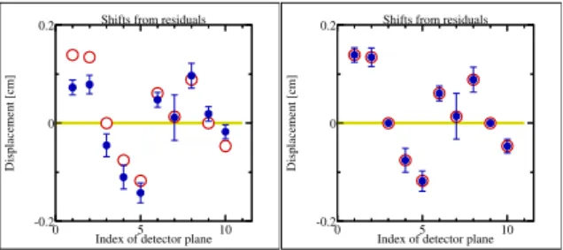
Fig. 1. Alignment of the planes of a toy detector. The true shifts are given by the large circles. Results of the histogram alignment after 30 iterations are shown by points with error bars, on the left after the first attempt with 10 free parameters, and on the right with two parameters fixed at zero.
2. Toy detector alignment
A popular alignment method in HEP is based on residual histograms. Tracks are fitted using a pre-liminary alignment. Histograms of hit residuals are generated and analysed, and the offsets observed in the histograms are used to adjust the alignment. This method is tested below in a simple MC study. A toy track detector is assumed with 10 drift chamber planes, 1 m high, 10 cm distance, no mag-netic field, with a nominal accuracy ofσ≈200µm and an efficiency= 90% (plane 7 with reduced ac-curacy and efficiency). The chambers are displaced vertically by a certain shift of ≈ 0.1cm. 10 000 tracks with a total of 82 000 hits are generated and available for alignment.
The first alignment attempt is based on the dis-tribution of hit residuals: a straight line is fitted to the track data, and the residuals (= measured ver-tical coordinate minus fitted coordinate) are his-togrammed, separately for each plane. The mean value of the residuals is taken as correction to the vertical plane position, and the procedure is re-peated iteratively. There are large changes in the first iteration, small changes in the second itera-tion, and almost no change afterwards. The result after 30 iterations is show in Figure 1 (left).
The reason for non-convergence to the true shifts is simple: two degrees of freedom are undefined, a simultaneous shift and an overall shearing of the planes. In a second attempt, the displacement of two planes (planes 3 and 9), assumed to be care-fully aligned externally, is fixed at zero. After large
changes in the first iteration there are smaller and smaller changes in the following iterations. The re-sult after 30 iterations in Figure 1 (right) shows that the method is converging, but rather slow, be-cause the determination of displacements is based on biased fits.
Can the bias of the track-fit results due to the initially unaligned detector be avoided by a differ-ent method? A correct approach would be the si-multaneous fit of the (global) alignment parame-terspglobal and all (local) track parametersqlocal, with the model
mi∼=f(qlocal,pglobal)i=q1local+q local
2 ·si+∆p
global
j
for the measured valuemi, where ∆pglobalj is the
shift for plane j. This is a linear least squares problem of 82 000 equations (measurements) and 20 010 parameters, which requires the solution of a linear equation with a 20010×20010 matrix. The special structure of the matrix however al-lows the reduction to an 8×8 matrix for the in-teresting plane-shift parameters, which are easily determined without iterations, if planes 3 and 9 are fixed at displacement = 0. This matrix reduc-tion is explained in Chapter 4. The full covariance matrix is available after the fit and shows that the standard deviations of the shifts are around 3µm. The method is easily extended to the tion of additional parameters e.g. the determina-tion of correcdetermina-tions ∆vdrift/vdrift of drift velocities for each plane, using the equations
mi∼=q1local+q local 2 ·si +∆pglobalj +`drift,i· ∆vdrift vdrift j
with a further reduction of the residuals. This im-provement would be rather difficult to obtain with a pure residual-based method.
3. Special alignment methods
Histogramming.The basic idea of the histogram method, already mentioned in the previous section, is to extract parameter corrections from the peak (or mean or median) of residual histograms. The advantage of this method is that almost no extra
Fig. 2. Plot of residuals as a function of azimuthal angle before (left) and after (right) alignment.
code is necessary and the histograms can be gener-ated fromn-tuples of the residuals. However, the residuals are taken from biased fits and no preci-sion alignment can be expected. In order to obtain convergence, many iterations would be necessary and therefore the method is extremely slow. The method is limited to those parameters which are directly accessible from residuals histograms. Fur-thermore it is not obvious how to fix undefined or badly defined degrees of freedom.
Residuals histograms can, however, be useful to detect large misalignments (see Figure 2) of cer-tain detectors, if also hits that are not assigned to the track are included in the histograms. The de-tection of very large local misalignments may be impossible otherwise.
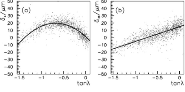
Parametrization of residual dependence.An interesting method has been used for the internal alignment of the SLD vertex detector[2]. Starting from tracks reconstructed in the central drift cham-ber, different types of tracking constraints were classified in the three planes of the vertex detec-tor. For each type of residuals a functional form was derived and fitted to the measured residuals accumulated inn-tuples (Figure 3). In total 2108 coefficients from 700 residual fits were determined. Taking into account in addition CCD shape correc-tions from the optical survey data of the CCD sur-faces and taking into account the covariance ma-trices of the residual fits, 866 alignment corrections were determined from 5026 coefficients of the resid-ual fits, using singular value decomposition (SVD) techniques for the least-squares fit minimization in
Fig. 3. Examples for residual fits in the SLD vertex detector alignment, here as a function of tanλ in a certain layer before the alignment [2].
a single step. With the aligned geometry a one-hit resolution of 4µm in both the rz and rφ planes was found, close to the true intrinsic CCD reso-lution, and the design performance was achieved. The post-alignment RMS of the residual distribu-tions was found to be around a factor of four im-proved over the pre-alignment RMS values. Alignment using a Kalman filter. A method for the estimation of alignment parameters dur-ing track reconstruction in parallel with the track parameter estimation using the Kalman filter has been studied [3]. After each track fit, the current alignment parameters are updated using an exten-sion of the standard Kalman filter, which is a re-cursive least squares method.
Equations for updating the alignment parame-ters p and their covariance matrixV, as well as for the parameters of trackkand their covariance matrixVk are derived, which decouple into
sep-arate systems of equations. The correction to the alignment parameters is given by
∆p=V DTW(m−f) .
The update requires the inversion of a matrix with the dimension of the measurement vectormas well as several matrix products:
W =Vmeas+HVkHT+DV DT
−1
, where Vmeas = covariance matrix of m, and D andH are the Jacobians of the track functionf
w.r.t. the alignment and track parameters. The resulting alignment, considered to be a sort oflocalalignment, gives the positions and orienta-tions of a set of detector elements with respect to a fixed set of reference detectors. Convergence has
been studied in a MC simulation with six detectors to be aligned. Occasional convergence to local min-ima cannot be excluded; this problem is solved by the introduction of annealing, gradually stepping up the weights of the observations in the course of the estimation process.
4. Matrix methods for alignment
There are large correlations between the align-ment parametersp, which specify the position and orientation of detector elements. The standard method for the determination of a large number of ncorrelatedparameters is the solution of a system of linear equations, derived from a least squares sum of residuals, which has to be minimized. Cor-rections ∆p are determined from the system of normal equations C∆p = b with a symmetric n×n matrix C and a n-vector b. The problem is characterized not only by the large value of n, but also by the large amount of data from many events that have to be employed in the procedure in order to get accurate estimates for∆p.
4.1. Alignment parameters of a planar sensor Six alignment parameters are required for a com-plete alignment of a planar sensor like a silicon pixel or strip detector. Coordinates and transfor-mations are as follows [4]. Local (sensor) coordi-natesq= (u, v, w), defined w.r.t. a sensor and used for track reconstruction, and the coordinatesr= (x, y, z) in the global detector system are related by the linear transformation
q=R(r−r0)
with a nominal rotation matrixR, and the nominal position vector r0. The origin of the (u, v, w) is at the center of the sensor; the u-axis along the precise coordinate and thev-axis along the coarse coordinate are in the sensor plane.
After alignment the transformation becomes
qaligned= (RγRβRα)R(r−r0)−∆q
with the correction vector ∆q = (∆u,∆v,∆w);
Rα,RβandRγ are rotation matrices, defined by
(small) angles of rotation ∆α, ∆βand ∆γaround theu-axis, the (new)v-axis and the (new)w-axis. In the small-angle approximation the correction matrix for rotation becomes
RγRβRα= 1 ∆γ −∆β −∆γ 1 ∆α ∆β −∆α 1 .
Usually not all parameters (∆u,∆v,∆w) and (∆α,∆β,∆γ) are well-defined and it may be bet-ter to use a sub-set or selected linear combinations of the six parameters.
4.2. Global degrees of freedom
It is a trivial fact, that e.g. a global translation of the whole detector has no influence on theχ2 of the track. Therefore, track residual minimiza-tion as the basic principle in detector alignment is not sufficient to fix all global degrees of freedom. Undefined or weakly defined global degrees of free-dom may introduce certain distortions, which do not affect track-fitχ2-values, but result in a bias of fitted track parameters. This has to be avoided. A general linear transformation with a transla-tion vector and a 3×3 matrixR
x0 y0 z0 = dx dy dz +R x y z ,
depends on 3 + 9 parameters; the matrix with 9 parameters can be decomposed into
– three rescaling factors fx, fy, fy,of coordinate
axes,
– three rotationsDx,Dy,Dzand
– three shearingsTxz,Tyz,Txy.
At least some of these linear-transformation pa-rameters have to be fixed in an alignment proce-dure. In addition, there are weakly defined non-linear transformations or deformations. Examples are: so-called clocking, i.e. a radius-dependent φ-shift, radial distortions, telescope effect by a radius-dependent z-shift, and sagitta effects [5]. Some of the effects can be reduced by the simulta-neous use of different data sets in the alignment. The clocking effect will be reduced by using tracks with a vertex constraint. Mass-constraints in two-particle decays reduce sagitta effects. The
tele-scope and sagitta effects are reduced or eliminated by the use of cosmics with magnetic field (large distance to interaction point) and without mag-netic field (zero curvature). Cosmics and beam halo muons improve the alignment by introduc-ing additional correlations between the alignment parameters. High-momentum tracks are preferred because of the larger predictive power compared to low-momentum tracks with large multiple scat-tering.
Alignment by tracks should be supplemented by the use of external information e.g. from sur-vey and Laser alignment. Fixing certain reference planes will improve the stability of the alignment fit. Undefined degrees of freedom can be avoided by adding equality constraint equations, e.g. zero global displacement in thexdirection
dx= X
i
∆xi= 0
or zero rotation of the whole detector. The stan-dard technique is to introduce a Lagrange mul-tiplier λ after linearization of the constraint
g(p) +gT·∆p= 0
with vectorg =∂g(p)/∂p, extending the matrix equation to
Cglobal g gT 0 ∆pglobal λ = bglobal −g(p) .
Another method is to modify the solution of the matrix equation: singular value decomposition or diagonalization methods allow to recognize weakly defined linear combinations and to remove their effect (see Section 5).
4.3. Global minimization
Global alignment is based on the residuals ob-tained from the measurement of a large number of tracks. The alignment parameterspare global pa-rameters. Parametersqk for track kare local pa-rameters. In the linear approximation the measure-ment equation for measuremeasure-mentmiof the track k
is written as mi∼=f(qlocal,pglobal)i +δlocali T ∆qlocalk +dglobali T ∆pglobal, (1) where f(qlocal,pglobal)
i is the track model
pre-diction for mi and dglobali and δ
local
i are the
derivative vectors w.r.t. to the global and the local parameters. For a given alignment, a sin-gle track fit for track k is performed by χ2 -minimization of the weighted sum of residuals ri = mi −f(qlocal,pglobalk )i using the current
alignment parameter values. The weightwi is the
inverse variance of the measurementmi.
Single track fit.The normal equations of the least squares solution for the track parameters are
Γk× ∆qk
= βk
(2) with the symmetric matrixΓk and the vectorβk,
given by the sums over all measurements of the trackk: Γk = X i wiδlocali δlocali T βk= X i wiriδlocali .
Track parameter corrections are obtained iter-atively by ∆qk = Γ−k1βk until the vector βk
becomes negligible. The covariance matrix of the track parameters after convergence isVk=Γ−k1.
Simultaneous alignment and track fit.The so-calledglobal χ2-function is the least squares sum over a large number of tracks from different data sets χ2= X data sets X events X tracks X hits wiri2 !!! , (3) which is minimized either with respect to the align-ment corrections∆ponly (solution I), or with re-spect to the corrections∆pandall track parame-tersqj (solution II).
The normal equations for theχ2-function (3) of the alignment parameters andalltrack parameters are given by C . . . Gk . . . . . . . GTk 0 Γk 0 . . . . × ∆p · · · ∆qk · · · = b · · · βk · · · (4)
wherekis the track index. SubmatrixC is a sym-metric n×n matrix (n = number of alignment parameters) and there are K·m additional rows and columns, ifKtracks with eachmparameters contribute. The complete matrix of Equation (4) is huge, and cannot be stored in memory.
In order to build-up the matrix of Equation (4) single tracks are fitted in a loop over all events from all data sets. Then×nmatrixCand then-vector
bof the (global) alignment parameters are formed, track by track, by a sum with contributions from all measurements; the update formulae are, for each track, C :=C+X i wid global i dglobali T (5) b:=b+X i wiridglobali . (6)
In addition, there is for each trackka rectangular n×mmatrixGk, which correlates the parameters
of trackkwith the alignment parameters. It is de-termined by a sum over all measurements of track k: Gk = X i wid global i δlocali T .
The matrix equation (4) cannot be solved di-rectly because of its size. Two methods for the de-termination of the corrections∆pof the alignment parameters are in use, which are described in the following.
Solution I. One possibility is to solve the huge system of linear equations (4) iteratively. First, all tracks are fitted using the current values of align-ment parameters to form the sums for C and b
and, ignoring the matricesGk, the linear system
C
× ∆p
= b
. (7)
is solved for alignment corrections ∆p. This method only takes into account the direct correla-tion between the different alignment parameters, whereas the complete correlations between the different alignment parameters, mediated by the tracks, are neglected. Therefore, the single-track fits and the solution of Equation (7) have to be repeated many times. Experience has shown that the iterative solution is converging, but many,
perhaps several hundred, iterations are necessary to reach the final solution.
Applications.The method has been used succes-fully in several experiments, e.g. [6]. In the align-ment of the upgraded vertex detector ofAlephat LEP2 [7] a global χ2 involving all 864 = 144×6 degrees of freedom is built, using single tracks and vertex constraints. Selected information is used from the outer tracking. Precise faces measure-ments are used to reduce the degrees of freedom, while allowing for parametrized distortions. The method is shown to provide accurate results, even with a limited number of events. 16 000 hadronic Zevents are used.
A sensor alignment with repeated track fitting and residual optimization has been developed for the CMS experiment by [4]. As described in Sec-tion 4.1, six parameters are required for one planar sensor. Within solution I, there are no correlations between different sensors, and therefore the solu-tion involves matrices whose dimension is at most 6×6. The method was applied in a precision sur-vey in a test beam setup with several silicon strip detectors. The performance has also been tested in a simulated two-layer pixel detector, with 144 sensors in layer 1 and 240 sensors in layer 2, each with 6 parameters. Only a few iterations were nec-essary in the case where all sensors of the second layer were fixed. In the case of only a single fixed sensor and all remaining 383 sensors misaligned, the number of iterations needed to reach a reason-able precision for the 2298 fitted parameters varied between 20 and 100.
Solution II.A non-iterative determination of the alignment parameters is possible due to the special structure of the huge matrix in Equation (4). As far as the alignment is concerned, Equation (4) can be reduced to an equation for the alignment parameters ∆p only, with a modified matrix C0
and vector b0. This method has been developed for theMillepedepackage [8] for alignment1. As before, a loop over all tracks is performed with 1 There are indications that this matrix-size reduction in
large least squares problems has been used in surveying already in the 19th century.
single track fits, and the contribution from each track is added: C0:=C0+X i widglobali dglobali T −GkVkGTk (8) b0:=b0+X i wirid global i −GkVkβk (9)
(usually the corrections to the vectorbare zero, be-cause the vectorsβkfor tracks are zero). No further information from single tracks has to be stored. The matrix update includes the information from the parameters of trackk. In particular, the com-plete correlations between the different alignment parameters are included. Finally, after accumula-tion of all informaaccumula-tion from all tracks the matrix equation
C0
× ∆p
= b0
(10) has to be solved. MatricesC0 and vectorsb0from several data sets can be simply added to get a combined result. The method allows to introduce equality constraints (see Chapter 4.2). The algo-rithm to solve large least squares problems in a sin-gle step (no iterations) and taking into account all correlations is general and can be applied to other problems with a large number of (global) parame-ters and a huge number of measurements with lo-cal parameters. In the alignment, a few iterations may be necessary to check the code, because of lin-ear approximations made in the track model, or because of the limited accuracy of the solution of the large system of linear equations. Another rea-son for iterations may be the removal of outliers, applying certain cuts which are tightened from it-eration to itit-eration.
Applications. The Millepede package is used in several experiments (H1(1997), [9], CDF(2001) [10], Hera-B) or is under test for others (CMS, LHCb, PHENIX, ZEUS). Starting from a differ-ent ansatz, essdiffer-entially the same method to reduce the matrix size was derived in the ATLAS align-ment group (convenor A. Hicheur); the conference report[5] describes tests in simulated experiments and contains several formulae for vertex and mass constraints etc.
A common alignment and detailed calibration was performed in the H1 experiment using the
RMS(residuals) vs drift
2000/11/28 17.38
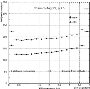
Fig. 4. Residuals as a function of the drift length in the H1 drift chamber. RMS values are reduced from 180µm to 125µm in the alignment withMillepede.
Millepedepackage for the silicon detector (two planes) and the drift chambers (56 planes), with a total of 1 400 parameters using 50 000 tracks [9]. For the two drift chambers, 14 global parameters representing an overall shift or tilt were introduced. Local variations of the drift velocityvdrift for cell halfs and layer halfs are observed and described by 180 + 112 corrections, which change with the HV configuration. For each group of 8 wires corrections toT0 are introduced (330 corrections). The result is shown in Figure 4, where the reduction of the mean track residuals from≈180µm to≈125µm is visible.
Because of CPU time and memory constraints the presentMillepedepackage is limited to align-ment problems with a numbernof parameters up to five or ten thousand. A new versionMillepede
IIis being developed applicable fornmuch larger
than 10 000. InMillepede II, the two tasks of the program are split. Accumulation of data is done by a small subprogram (Mille) inside the user pro-gram and the solution is determined in a stand-alone program (Pede). An efficient sparse-matrix storage scheme is dynamically defined and differ-ent solution algorithms (see Chapter 5) are avail-able. The solution is easily tested under different conditions using the accumulated data. Tests on
a standard PC with 25 000 parameters from one million tracks took less than one hour.
5. Numerical linear algebra
In matrix methods the corrections∆pfor align-ment parameters are determined by the solution of matrix equations (7) and (10) with a large n×n matrixC. Double precision storage for matrix and vector is important already in the accumulation phase. It is not a-priori clear whether a solution with acceptable accuracy can be obtained. The ac-curacy depends on thealgorithmand on thedata: 1. Algorithm: With a stable algorithm, the com-puted solution is the exact solution of a nearby problem. Gaussian Elimination with restricted scan on the diagonal for the next pivot element is considered to be a stable algorithm for posi-tive definite matrices.
2. Data: The system is called ill-conditioned, if small changes in the data can cause large changes in the solution. This behaviour is caused by vari-ables which are undefined or poorly defined or strongly correlated; all components of the solu-tion are affected in this case. Ill-condisolu-tioning can be detected by small eigenvalues of the matrix and by global correlation coefficients close to 1. Re-definition of the alignment parameters may improve the condition of the system.
Matrix and vector should be appropriately scaled with consistent units in data and variables, in or-der to reach similar precision for all elements. A large fraction of the memory will often be used for the matrix; special storage techniques for symmet-ric matsymmet-rices, band matsymmet-rices and sparse matsymmet-rices in general reduce the required space. Most algorithms can workin-space, i. e. no extra space is required for the inverted or decomposed matrix. Four solu-tion methods are listed below.
Solution with matrix inversion.The standard method is the Gauss algorithm with pivot selec-tion of the diagonal, with a computing time∝n3. Problems withn= several thousand are solved on a standard PC within a time of the order of one hour. In practice, often at least a few parameters are badly defined (dead or inefficient channels) and
standard matrix routines will fail. A simple method to avoid such problems is to stop the inversion if no acceptable pivot is found, i.e. the largest possible submatrix is inverted with accurate results for the related parameters; the corrections for the remain-ing parameters are set to zero (subroutine SPINV in Millepede [8]).
An advantage of the method is that all variances and covariances are available with the inverse ma-trix, which is the covariance matrix for parameters:
V =C−1. Theglobal correlation coefficient ρj
ρj = s
1− 1
(V)jj·(C)jj
can be calculated and gives a measure of the total amount of correlation between thej-th parameter andallother variables. It is the largest correlation between thej-th parameter and every possible lin-ear combination of all the other variables and has a range from 0 to 1. Values of the global correla-tion coefficient close to 1 mean a large correlacorrela-tion and may indicate that too many partially redun-dant parameters were introduced. The accuracy of matrix inversion is reduced in this case.
Singular value decomposition and Diagonal-ization.These algorithms allow to recognize sin-gularity or near-sinsin-gularity of the matrix by the de-termination of singular values or eigenvalues, and this allows to ignore the corresponding linear com-binations of parameters.
Diagonalization is the decomposition C =
U DUT with D diagonal (diagonal elements are the eigenvectorsλj), and matrixU square and
or-thogonal withU UT=UTU =1. The inverse is
C−1=U D−1UT. The decomposition algorithms are iterative, with a computing time≈ 10 times larger than for inversion, and additional space is needed for the n×n matrix U. The solution of
C∆p=bcan be written in the form ∆p=U diag 1 λi UTb .
Insignificant linear combinations, which could produce distortions of the alignment, indicated by small eigenvalues, are suppressed by setting 1/λi = 0 in the above formula for eigenvalues
λi = 0 or small. This method is tested in the
of the eigenvalues, and those singular modes are suppressed to avoid potential distortions of the detector.
Another solution is to define a vectorq by
q= diag 1 √ λi UTb
and to compute the solution∆pby ∆p=U diag 1 √ λi q.
By construction, the vectorqhas a covariance ma-trix V[q] = 1, and this allows to recognize and suppress insignificant contributions, recognized by a small value of|qi|.1.
Generalized minimal residual method (GM-RES). The fraction of non-zero off-diagonal ele-ments in the large matrix of a typical alignment problem is often rather small, of the order of a few percent. The approximate solution of a very large system of linear equations with a sparse matrix can be obtained by a certain algorithm for a quadratic minimization problem, in analogy to the method of conjugate gradients. One example isMINRES[11], designed to solve
C ∆p=b or min ||C ∆p−b||2, whereCis a symmetric matrix of logical sizen×n, which may be indefinite and/or singular, very large and sparse. The matrix is accessedonly by means of a subroutine call which must return the prod-ucty=Cxfor any given vectorx. This iterative solution is faster by several orders of magnitudes compared to matrix inversion.
An example of a compact storage, optimized for the above product, is the row-index sparse stor-age [12] with two arrays of (n+qn(n−1)/2 + 2) words (q = fraction of non-zero off-diagonal ele-ments), one for real numbers and one for integers. 512 Mbytes of memory are sufficient for a matrix withn= 100 000 for a value ofqclose to 1%. Cholesky decomposition.The Cholesky decom-positionC =LDLTof the symmetric matrix C
is numerically extremely stable, and can be made in-space; matrix L is a left unit triangular ma-trix (diagonal elements =1) and D is a diagonal matrix. The solution of C∆p=LDLT∆p=
bis obtained by forward and backward substitu-tion. With a clever ordering of parameters the ma-trixCof alignment problems can be approximated by aband matrix. An important property of the Cholesky decomposition is the fact that for band matrices with band-widthmthe band structure is kept in this decomposition and the computing time is only∝ m2×n. The subset of elements of the inverse matrix corresponding to the band of the original matrixC can be calculated quickly. Fast methods exist also for variable-bandwidth matri-ces (sky-linematrix), and for bordered band matri-ces (arrow matrix), where the border (additional full rows and columns) can for example be due to Lagrange multiplier constraints.
Several matrix algebra libraries exist, e.g. GNU Scientific Library (GSL), Numerical Algorithms Group (NAG), BLAS (Basic Linear Algebra Sub-programs), and LAPACK (Linear Algebra PACK-age).
6. Alignment strategies and summary Alignment problems withn= several thousand parameters have been successfully solved, either using rather specialized methods, by algorithms re-quiring a large number of iterations or by global χ2-minimization in a single step. The experience has shown that the integration of alignment into the reconstruction code and the use of fast align-ment algorithms is of advantage; it allows a rou-tine check of the time stability of alignment. The simultaneous use of several or all available types of events, physicsand background events, and of single tracks and tracks with vertex and invariant-mass constraints can reduce or avoid potential dis-tortions.
The next generation of experiments, e.g. the AT-LAS and the CMS experiment at the LHC, have a huge number of independent sensors with an excel-lent spatial resolution from about 10µm to about 50µm. An alignment precision for all sensors, with up to n = 105 parameters (CMS experiment at LHC), below the intrinsic resolution is required to get the necessary measurement accuracy for the physics program at the LHC.
The best and most suitable strategy for this large number of parameters is unknown at present. Both experiments have formed alignment working groups, where the impact of mis-alignment is stud-ied [13] and different methods of alignment are de-veloped in parallel and compared. The algorithms under study are rather similar in the two experi-ments. Both, simple straightforward and perhaps robust methods and advanced methods are stud-ied in the ATLAS Alignment group (convenor A. Hicheur):
– Localχ2alignment: modules aligned on an indi-vidual basis with 6×6-matrices, iteratively us-ing the alignment and refittus-ing tracks,
– Global χ2 alignment: simultaneous alignment and track fits with the full Pixel + SCT Barrel and Endcaps ([5]),
– Alignment with overlaps: relative module to module misalignment determined from overlap residuals,
as well as in the CMS Alignment group (coordina-tor O. Buchm¨uller)
– Sensor alignment by tracks: iterative procedure that considers individual measurement devices with 6×6-matrices (not taking into account cor-relations between measurement devices) [4] [14], – Millepede II:upgraded version of Millepede; – Kalman filter alignment [3].
Some theoretical progress in alignment would be welcome to find a general strategy to suppress un-wanted distortions, which can be used even for a very large value ofn. However, there is confidence that good alignment strategies will be available at the time when they will be needed.
References
[1] National Institute of Standards and Technol-ogy, NIST/SEMATECH e-Handbook of Statis-tical Methods (2005)
www.itl.nist.gov/div898/handbook/ [2] D. J. Jackson, D. Su and F. J. Wickens, Internal
alignment of the SLD vertex detector using a matrix singular value decomposition technique.
Nuclear Instr. Methods A510, 233–247 (2003) [3] R. Fr¨uhwirth, T. Todorov and M. Winkler, Es-timation of detector alignment parameters us-ing the Kalman Filter with annealus-ing, J.Phys. G: Nucl. Part. Phys.29, 561–574 (2003) [4] V. Karim¨aki, A. Heikkinen, T. Lamp´en and T.
Lind´en, Sensor alignment by tracks, CMS Con-ference Report CHEP03, La Jolla, California, March 24-28, 2003
[5] P. Br¨uckman de Renstrom, S. Haywood: Least squares approach to the alignment of the generic tracking system, Phystat2005, Ox-ford.
[6] A. Sopczak, Alignment of the D0 Vertex De-tector, these proceedings.
[7] A. Bonissent et al., Alignment of the upgraded VDET at LEP2, ALEPH 97-116, 1997
[8] V. Blobel, Linear Least Squares Fits with a Large Number of Parameters, (2000), http://www.desy.de/~blobelincluding For-tran code.
[9] V. Blobel and C. Kleinwort: A New Method for the High-Precision Alignment of Track De-tectors, Procedings Phystat2002, Durham, arXiv-hep-ex/0208021
[10] R. McNulty et al., A Procedure for the Soft-ware Alignment of the CDF Silicon System, CDF/DOC/TRACKING/GROUP/5700(2001) [11] C. C. Paige and M. A. Saunders, Solution of
sparse indefinite systems of linear equations, SIAM J. Numer. Anal.12(4), 617 – 629 (1975) [12] W. H. Press, S. A. Teukolsky, W. T. Vetter-ling, B.P. Flannery, Numerical Recipes – The Art of Scientific Computing, Cambridge Univ. Press, 1999
[13] N. De Filippis, Impact of CMS Tracker Mis-alignment on Track and Vertex Reconstruc-tion, these proceedings.
[14] T. Lamp´en, General Alignment Concept of CMS, these proceedings.