CIRJE Discussion Papers can be downloaded without charge from: http://www.e.u-tokyo.ac.jp/cirje/research/03research02dp.html
Discussion Papers are a series of manuscripts in their draft form. They are not intended for circulation or distribution except as indicated by the author. For that reason Discussion Papers may not be reproduced or distributed without the written consent of the author.
CIRJE-F-200
Finite Sample Distributions of the Empirical
Likelihood Estimator and the GMM Estimator
Naoto Kunitomo Yukitoshi Matsushita The University of Tokyo
March 2003 Revised: December 2003
Finite Sample Distributions of the Empirical Likelihood
Estimator and the GMM Estimator
∗Naoto Kunitomo† and Yukitoshi Matsushita January 2003 November 2003 (2nd Revision) Abstract
The distributions of the Maximum Empirical Likelihood (MEL) estimator and the Generalized Method of Moments (GMM) estimator for the coefficient of one en-dogenous variable in a linear structural equation are evaluated numerically. Tables and figures are given for enough values of the parameters to cover most of interest. Comparisons of the distributions of the MEL estimator and the GMM estimator with their asymptotic expansions are made. We find that the MEL estimator does not have any moments of positive integer orders and careful analyses are needed to use its bias and mean squared error because usually they do not exist.
Key Words
Finite Sample Properties, Maximum Empirical Likelihood, Generalized Method of Mo-ments, Econometric Structural Equation, Asymptotic Expansions, Non-existence of Exact Moments
JEL Code: C13, C30
∗This is a revised version of Discussion Paper CIRJE-F-200, Graduate School of Economics,
Univer-sity of Tokyo. We thank Professor Theodore W. Anderson for useful comments to the earlier version of this paper.
†Graduate School of Economics, University of Tokyo, 7-3-1 Hongo, Bunkyo-ku, Tokyo 113-0033,
1. Introduction
The study of estimating a single structural equation in econometric models has led to develop several estimation methods as the alternatives to the least squares esti-mation method. The classical examples in the econometric literatures are the limited information maximum likelihood (LIML) method and the instrumental variables (IV) method including the two-stage least squares (TSLS) method. See Anderson, Kunit-omo, and Sawa (1982) on the studies of their finite sample properties, for instance. Also the generalized method of moments (GMM) estimation, originally proposed by Hansen (1982), has been often used in econometric applications. The GMM estimation method is essentially the same as the estimating equation (EE) method originally developed by Godambe (1960) which has been mainly used in statistical applications.
In addition to these estimation methods, the maximum empirical likelihood (MEL) method has been proposed and has gotten some attention recently in the statistical and econometric literatures. It is probably because the MEL method gives an asymptoti-cally efficient estimator in the semi-parametric sense and also improves the serious bias problem known in the estimating equation (EE) method or the generalized method of moments (GMM) method. See Owen (2001), Qin and Lawless (1994), Kitamura (1997), and Kitamura et. al. (2001) on the details of the MEL method.
For sufficiently large sample sizes the GMM estimator and the MEL estimator have approximately the same distribution, but their exact distributions can be quite different for the sample sizes occurring in practice. The main purpose of this study is to give numerical information to determine the small sample properties of the exact cumulative distribution functions (cdf’s) of the MEL estimator and the GMM estimator for a wide range of parameter values. Since it is quite difficult to obtain the exact densities and cdf’s of these estimators, this information makes possible the comparison of properties of two alternative estimation methods. Advice can be given as to when one is preferred to the other. In this paper we use the classical estimation setting of a linear structural equation when we have a set of instrumental variables in econometric models. It is our intention that we can make precise comparison of alternative estimation procedures in the possible simplest case which has many applications.
Another approach to the study of the finite sample properties of alternative estima-tors is to obtain asymptotic expansions of their exact distributions in the normalized forms. As noted before, the leading terms of their asymptotic expansions are the same, but the higher-order terms are different. Kunitomo (2002), Kunitomo and Matsushita (2003) have recently derived the asymptotic expansions of the distributions of the MEL estimator and the GMM estimator for the linear structural equation case under a set of assumptions. Newey and Smith (2001) has obtained some expressions of the asymp-totic bias and the asympasymp-totic mean squared errors for a class of estimators including the MEL estimator and GMM estimator for the general nonlinear case.
It should be noted, however, that the mean and the mean squared errors of the exact distributions of estimators are not necessarily the same as the mean and the mean squared errors of the asymptotic expansions of the distributions of the estimators. In fact we shall show that the MEL estimator does not posses any moments of positive integer order under a set of reasonable assumptions. Although the analyses of bias and the mean squared errors of the MEL estimator based on Monte Carlo experiments have been reported in some studies, we suspect that many of them are not reliable. Therefore
instead of moments we need to investigate the exact cumulative distribution of the MEL estimator directly in a systematic way and it is precisely what we are going to explain in this paper. The problem of non-existence of moments had been already discussed in the econometric literatures because the limited information maximum likelihood (LIML) estimator does not have any moments of positive integer orders under a set of reasonable assumptions. For instance, see Phillips (1980) and Phillips (1983) on the details of the finite sample properties of the traditional econometric estimators in the parametric framework.
In Section 2 we state the formulation of models and two estimation methods of unknown parameters. In Section 3 we shall give tables and figures of the distributions of the estimators and then in Sections 4 we shall discuss the small sample properties of two estimators. In Section 5 we show the non-existence of exact moments of the MEL estimator under a set of assumptions. Finally, some conclusions will be given in Section 6. Tables and Figures are gathered in Appendix.
2. Estimating a Single Structural Equation by the Empirical Likelihood Method
Let a single linear structural equation in the econometric model be given by
y1i = (y2i,z1i)( βγ ) +ui (i= 1,· · ·, n), (2.1)
wherey1i andy2iare 1×1 andG1×1 (vector of) endogenous variables,z1i is aK1×1 vector of exogenous variables,θis ap×1 (p=K1+G1) vector of unknown parameters, and {ui} are mutually independent disturbance terms withE(ui) = 0 (i= 1,· · ·, n). We assume that (2.1) is the first equation in a system of (G1+ 1) structural equations in which the vector of 1 +G1 endogenous variables yi = (y1i,y2i) and the vector of
K (=K1+K2) exogenous variables{zi} including {z1i} are related linearly with the conditionn > K .The set of exogenous variables{zi}are often called the instrumental variables and we can write the orthogonal condition
E[uizi] =0 (i= 1,· · ·, n). (2.2)
Because we do not specify the equations except (2.1) and we only have the limited information on the set of exogenous variables or instruments, we only consider the limited information estimation methods. Furthermore, when all structural equations in the econometric model are linear, the reduced form equations ofyi = (y1i,y2i) can be defined by
yi =Πzi+vi (i= 1,· · ·, n), (2.3)
wherevi= (v1i,v2i) is a 1×(1 +G1) disturbance terms withE[vi] =0 and
Π= (π1,Π2) = ( π11 Π12
π21 Π22 ) (2.4)
is a (K1+K2)×(1 +G1) (K = K1+K2) partitioned matrix of the reduced form coefficients. By multiplying (1,−β) to (2.3) from the left-hand side, we have the relationui =v1i−βv2i(i= 1,· · ·, n) and the restriction
(1,−β)Π = (γ,0) . (2.5)
The maximum empirical likelihood (MEL) estimator for the vector of parametersθ in (2.1) is defined by maximizing the Lagrangian form
L∗ n(λ, θ) = n i=1 logpi−µ( n i=1 pi−1)−nλ n i=1 pizi[y1i−βy2i−γz1i], (2.6)
whereµ and λ are a scalar and aK×1 vector of Lagrangian multipliers, andpi (i= 1,· · ·, n) are the weighted probability functions to be chosen. It has been known (see Qin and Lawles (1994) or Owen (2001)) that the above maximization problem is the same as to maximize Ln(λ, θ) =− n i=1 log{1 +λzi[y1i−βy2i−γz1i]}, (2.7)
where we have the conditions ˆµ=n ,and
[npˆi]−1 = 1 +λzi[y1i−βˆy2i−ˆγz1i]. (2.8)
By differentiating (2.7) with respect to λ and combining the resulting equation with (2.8), we have the relation
n i=1 ˆ pizi[y1i−βy2i−γz1i] = 0 (2.9) and ˆ λ= [ n i=1 ˆ piu2i( ˆθ)zizi]−1[1 n n i=1 ui( ˆθ)zi], (2.10)
where ui( ˆθ) =y1i−βˆy2i−γˆz1i and ˆθ = ( ˆβ,ˆγ) is the maximum empirical likelihood (MEL) estimator for the vector of unknown parametersθ .
In the actual computation we first minimize (2.7) with respect toλand then the MEL estimator can be defined as the solution of constrained maximization of the criterion function with respect to θ under the restrictions 0< ≤pi < 1 (i= 1,· · ·, n),where we take a sufficiently small (positive) . Alternatively, from (2.7) the MEL estimator of{θ} can be written as the solution of the set of p equations
ˆ λn i=1 ˆ pizi[−(y2i,z1i)] = 0 , (2.11) which implies [ n i=1 ˆ pi( yz2i 1i )z i][ n i=1 ˆ piui( ˆθ)2zizi]−1[n1 n i=1 zi y1i] (2.12) = [ n i=1 ˆ pi( yz2i 1i )z i][ n i=1 ˆ piui( ˆθ)2zizi]−1[ 1 n n i=1 zi(y2i,z 1i)]( ˆ β ˆ γ ).
On the other hand, the GMM estimator ofθ = (β, γ) can be given by the solution of the equation 1 [1 n n i=1 ( y2i z1i )z i][n1 n i=1 ui( ˆθ)2zizi]−1[n1 n i=1 ziy1i] (2.13) = [1 n n i=1 ( y2i z1i )z i][n1 n i=1 ui( ˆθ)2zizi]−1[n1 n i=1 zi(y2i,z1i)]( ˆ β ˆ γ ),
where ˆθ is a consistent initial estimator ofθ .
By this representation the GMM estimator can be interpreted as the empirical like-lihood estimator when we use the fixed probability weight functions as pi = n1 (i = 1,· · ·, n). In the actual computation we use the two-step efficient GMM procedure ex-plained by Page 213 of Hayashi (2000), which seems to be standard in many empirical analyses.
We shall consider the situation that the disturbances are homoscedastic random variables although they can be conditionally heteroscedastic. Let the standardized error of estimators be in the form of
ˆ
e=√n( βˆ−β ˆ
γ−γ ) ,
(2.14)
where ˆθ = ( ˆβ,ˆγ) and θis the vector of unknown coefficient parameters. Under a set of regularity conditions2 , the inverse of the asymptotic variance-covariance matrix of the asymptotically efficient estimators is given by
Q−1=σ−2DMD, (2.15) where D = [Π2 ,( IK1 O )], (2.16) M = plimn→∞n1 n i=1 zizi . (2.17)
provided that E(u2i) = σ2 (> 0),the constant matrix M is positive definite, and the rank condition
rank(D) =p(=G1+K1). (2.18)
These conditions assure that the limiting variance-covariance matrixQis non-degenerate. The rank condition implies the order condition
L=K−p≥0, (2.19)
which has been called the degrees of over-identification.
In the standard linear setting it is possible to obtain the convergence in probability thatnpˆi →1 (i= 1,· · ·, n) whenn→ ∞ as Owen (1990) and Qin and Lawless (1994)
1 This formulation is different from the original one. See Hayashi (2000) on the details of the GMM
estimation method.
2 See Qin and Lawles (1994) on the details of sufficient conditions for the i.i.d. case, which can be
have shown. Then the MEL estimator and the GMM estimator are asymptotically equivalent and their asymptotic variance-covariance matrix is given by Q . However, this does not necessarily mean that their finite sample distributions are similar.
It is also straightforward to treat the multiple equation case in the present formu-lation. If we have m equations, let ui = (u(ij)) be a sequence of m×1 vectors of disturbance terms. Then we write the orthogonal conditions as
E[ui ⊗zi] =0 (i= 1,· · ·, n), (2.20) and ui(j)=y(1ji)−(y2(ji),z(1ji))( β(j) γ(j) ) (j= 1,· · ·, m), (2.21)
wherey2(ji) andz(1ji) areG(1j)×1 andK1(j)×1 vectors of variables, respectively, andβ(j) and γ(j) are the corresponding coefficient vectors. It is clear that the MEL estimaton problem of the multiple equation case is parallel to the single equation case as we have discussed with some complications in notation. Also it has been known that many econometric models for panel data can be reduced to the above multiple equation form. ( See Section 3 of Arellano and Honor´e(2001) or Chapter 4 of Hsiao (2003) on the related discussions, for instance.)
3. Evaluation of Distributions and Tables 3.1 Parameterizations
The estimation method of the cdf’s of estimators we have used in this study is based on the simulation method since their analytical properties are difficult to be investi-gated directly. In order to describe our estimation method, we need to introduce some notations which are similar to the ones used by Anderson et. al. (1982) for the ease of comparison. We shall concentrate on the comparison of the estimators of the coefficient parameter on the endogenous variable whenG1 = 1 in this section.
LetMbe aK×Kmatrix given by (2.17) and we partition the nonsingular matrix
Minto (K1+K2)×(K1+K2) sub-matricesM= (Mij) (i, j= 1,2).Also let aK2×K2 matrix
M22.1=M22−M21M−111M12. (3.1)
When the disturbance terms are homoscedastic, the (1,1) element of the inverse of the asymptotic variance-covariance matrixQ−1 is given by
Q11= 1
σ2Π22M22.1Π22.
By multiplyingn(the sample size) to this quantity, we rewrite 1
σ2Π22A22.1Π22, (3.2)
where we have used the notationA22.1=nM22.1 .This corresponds to the parameteri-zation adopted by Anderson et. al. (1982) on the study of the finite sample properties of the LIML and TSLS estimators in the classical parametric framework. In the rest
of our study we shall consider the finite sample distribution for the coefficient of the endogenous variable β because of the simplification. We expect that we have similar results on other coefficients parameters.
We consider the distributions of the normalized estimator as
Π22A22.1Π22
σ ( ˆβ−β).
(3.3)
The distribution of (3.3) for each estimator depends on the parameterization of the underlying econometric model in a rather complicated way. For the easiness of the re-sulting interpretations we have adopted the notations used by Anderson et. al. (1982), that is,L=K−p , δ2 = Π 22A22.1Π22 ω22 , (3.4) and α= ω22β−ω12 |Ω|1/2 . (3.5)
In these notationsL is the difference between the number of restrictions and the num-ber of parameters, which is the degrees of over-identification. In applied econometric analyses L can be very large in some circumstances including Panel Data analyses. The parameterα can be interpreted intuitively by transforming it into ρ=−α/√1 +α2 . Then we can rewrite
ρ= ω12−ω22β
σ√ω22 ,
which is the correlation coefficient between two random variables ui and v2i (or y2i). It has been often called the coefficient of simultaneity in the structural equation of the simultaneous equations system. Finally the non-centrality parameterδ2plays a key role in the subsequent analysis. The numerator of δ2 is the additional explanatory power due toy2ioverz1i in the structural equation and the denominator is the error variance of y2i . Therefore δ2 determines how well the equation is defined in the simultaneous equations system.
3.2 Simulation Procedures
By using a set of Monte Carlo simulations we can obtain the empirical cdf’s of the MEL and GMM estimators for the coefficient of the endogenous variable in the structural equation of our interest. First, we consider the case when both the disturbances and the exogenous variables are normally distributed. We generate a set of random numbers by using the two equations system
y1i =y2iβ(0)+z1iγ(0)+ui , (3.6)
and
y2i =ziπ2(0)+v2i, (3.7)
where zi ∼ N(0,IK), ui ∼ N(0,1), v2i ∼N(0,1) (i= 1,· · ·, n),and we set the true values3 of parametersβ(0) =γ(0)= 0.We have controlled the values ofδ2 by choosing
3 In order to examine whether our results strongly depend on the specific values of parameters
β(0)=γ(0)= 0, we have done the several simulations for the values ofβ(0)= 0 andγ(0)= 0.These
a real value of c and setting π2(0) = c(1,· · ·,1) . The model we have used has been restricted to the special case whenG1 =K1 = 1 because in general it takes prohibitively long computational time to estimate the empirical cdf of the MEL estimator when the number of parameters included the equation (3.6) is large. For each simulation we have generated a set of random variables from the disturbance terms and exogenous variables. In the simulation the number of repetitions were 5,000 and we consider the representative cases when the combination of the underlying quantities are such as
n= 50,100,300, L= 3,10,20,30, α= 0.0,1.0,5.0,and δ2 = 30,50,100,300. In order to investigate the effects of non-normal disturbances on the distributions of estimators, we took two cases when the distributions of the disturbances are skewed or fat-tailed. As the first case we have generated a set of random variables (y1i, y2i,zi) by using (3.6), (3.7), and ui =−χ 2 i(3)√−3 6 , (3.8)
where χ2i(3) are χ2−random variables with the 3 degrees of freedom. As the second case, we took the t-distribution with 5 degrees of freedom for the disturbance terms. 3.3 Tables and Figures
The empirical cdf’s of estimators are consistent for the corresponding true cdf’s. In addition to the empirical cdf’s we have used a smoothing technique of cubic splines to estimate the cdfs’ and their percentile points. The distributions are tabulated in the standardized terms, that is, of (3.3), mainly because this form of tabulation makes comparisons and interpolation easier. The tables includes the three quartiles, the 5 and 95 percentiles and the interquartile range of the distribution for each case. The estimators which we wish to compare (the MEL estimator with the GMM estimator), have the same asymptotic distribution. Therefore, the limiting distributions of (3.3) areN(0,1) asn→ ∞in all cases. We consider the normalized distributions because it is often easy to make comparisons.
We have summarized our results on the cdf’s of two estimators as Tables 1-6, which are the normal disturbance cases.
3.4 Accuracy of the Procedures
To evaluate the accuracy of our estimates based on the Monte Carlo experiments, we compared the empirical and exact cdf’s of the Two-Stage Least Squares (TSLS) estimator, which corresponds to the GMM estimator given by (2.13) when ˆu2i is replaced by a constant (namelyσ2), that is, the variance-covariance matrix is homoscedastic and known. The exact distribution of the TSLS estimator has been studied and tabulated extensively by Anderson and Sawa (1979).
We have chosen two cases among many and reported the exact cdf of the TSLS estimator, our estimate of its cdf, and their differences in Table 9 and Table 10. The differences are less than 0.005 in most cases and the maximum difference between the exact cdf and its estimates is about 0.008. Hence we have found that our estimates of the cdf’s are quite accurate and we have enough accuracy with two digits at least. This does not necessarily mean that the simulated moments such as the mean and the mean squared error in simulations are reliable as the same manner by the reason indicated in the last part of Introduction.
4. Discussions on Distributions
4.1 Distributions of the MEL Estimator
The distributions are tabulated in standardized terms, that is, of (3.3). The asymp-totic standard deviation (ASD) of ˆβ is given by
σ δ√ω22 = √ 1 +α2|Ω| δω22 . (4.1)
The spread of the distribution of the un-standardized estimator increases with|α|and decreases with δ . Since the GMM estimator which we wish to compare the MEL estimator has the same asymptotic standard deviation and in the remainder of the discussion we consider the normalized distributions as tabulated. For α = 0, the densities are close to symmetric. As α increases there is some slight asymmetry, but the median is very close to zero. For givenα, L,and n,the lack of symmetry decreases asδ2 increases. For givenα, δ2,andn, the asymmetry increases with L .
The main finding from Tables is that the distributions of the MEL estimator are roughly symmetric around the true parameter value and they are almost median-unbiased. This finite sample property does hold even when L is faily large. On the other hand, the distributions of the MEL estimator have relatively long tails. As δ2 → ∞, the distributions approachN(0,1); however, for small values ofδ2 there is an apprecia-ble probability outside of 3 or 4 ASD’s. As δ2 increases, the spread of the normalized distribution decreases. For given α,L,and δ2,the spread decreases asnincreases and it tends to increase withLand decrease with α . These observations about the spread agree with the asymptotic expansion of the cdf of the MEL estimator.
When the disturbances are normally distributed with some additional regularity conditions, it is possible to obtain the asymptotic expansion 4 of the distribution function in a compact form, which is given by
(4.2) P( Π22A22.1Π22 σ ( ˆβMEL−β)≤x) = Φ(x) +{−αµx2−21µ2[(ν+L)x+ (1−2α2)x3+α2x5]}φ(x) +O(µ−3),
where µ2 = (1 +α2)δ2 and Φ(·) and φ(·) are the cdf and the density function of the standard normal distribution, respectively. In the above expression the parameterν is defined by (4.3) ν =η(1 +α 2 ω22 )(1,0 )Q−111QNQQ−111(1,0) ,
4 The formulae of (4.2) and (4.7) are the results of lengthy and laborious derivations and the details
of the asymptotic expansions of the distribution functions of non-parametric (or semi-parametric)
estimators are reported in Kunitomo and Matsushita (2003). (4.5) and (4.8) are valid when µ3 =
E(u3i) = 0 with regularity conditions, but η= 2 +κin (4.2) and (4.6) while η= 2−κin (4.7) and (4.9) withκ(=E(u4i)/σ4−3) being the 4-th order cumulant.
where we use the notationsη = 2 (for the normal disturbance case),Q11=σ2(Π22 M22.1Π22)−1, theK×K matrix (4.4) N=plimn→+∞nσ12 n i=1 ziziM−1/2P¯EM−1/2zizi ,
and ¯PE =Ip−EQE is the projection operator for E= (1/σ)M1/2D.
We note that the asymptotic expansion in (4.2) was made in terms ofµ−1 under the situation when the noncentrality parameterδ2(orµ2) is proportional to the sample size and we have the condition of (2.17). Then (4.2) can be equivalently rewritten as the asymptotic expansion with respect to the standard normal distribution, the terms of
O(n−1/2),and the terms ofO(n−1).We report only the results in this situation because it can be regarded as the standard case and other cases can be similarly developed.
By using (4.2), the asymptotic mean (AMn) and the asymptotic mean squared errors (AMSEn) are defined as the mean and the mean squared errors based on the asymptotic expansion to orders O(δ−1) and O(δ−2), respectively. Afer some calcula-tions, they are given by
(4.5) AMn( ˆβMEL) = αµ = δ√ α 1 +α2 , and
(4.6) AMSEn( ˆβMEL) = 1 +µ12[ν+L+ 3 + 9α2], where we have the notation µ2 = (1 +α2)δ2 .
In the more general disturbance case the formula for AMn does not depend on any higher order moments and is not changed. However, in that case the formula for
AMSEndoes depends on the fourth order cumulant and there is an extra term in the order O(µ−2). Newey and Smith (2001) has mentioned to the first point in the more general nonlinear case although they used different notations.
The parameter ν in (4.2) is the key quantity in the semi-parametric estimation of econometric models. This term appears because we estimate the conditional variance-covariance matrix C∗n= 1 n n i=1 E[u2i|zi]zizi ,
which has been incorporated in the MEL estimation method when we denote the con-ditional variance byE[u2i|zi].
When we dropν in (4.2), the resulting formula of (4.2) is identical to the asymptotic expansion of the distribution function of the LIML estimator reported in Anderson (1974) and Fujikoshi et. al. (1982). Hence it can be interpreted as the effect due to the non-parametric estimation of a structural equation.
4.2 Distributions of the GMM Estimator
We have given tables of the distributions of the GMM estimator. The finite sample properties of the distributions approximately agree with the asymptotic expansions of the distribution functions and their moments. When the disturbance terms are
normally distributed, the asymptotic expansion of the distribution function of the GMM estimator can be given by
(4.7) P( Π22A22.1Π22 σ ( ˆβGMM−β)≤x) = Φ(x) +{−αµ(x2−L)−2µ12[(ν+L2α2−L)x+ (1−2(L+ 1)α2)x3+α2x5]}φ(x) +O(µ−3) .
Then by using (4.7) the asymptotic mean (AMn) and the asymptotic mean squared errors (AMSEn) of the GMM estimator are (up to ordersO(δ−1) andO(δ−2), respec-tively) given by (4.8) AMn( ˆβGMM) =−(L−1)α µ = −(L−1)α δ√1 +α2 , and (4.9) AMSEn( ˆβGMM) = 1 + 1 µ2[ν−(L−3)−4(L−2)α2+ (L−1)2α2]. We note that in the general disturbance case AMn of ˆβGMM depends on the third order moments of the disturbances terms and there is an extra term in (4.8) for the non-norma case. AlsoAMSEn of ˆβGMM depends on the fourth order moments. These facts could be seen by using the same arguments as Kunitomo and Matsushita (2003). Theν terms in (4.7) and (4.9) are of the same form as the corresponding term in (4.2) and (4.6). It can be interpreted as the effect due to non-parametric GMM estimation in our setting. When we drop ν in (4.7), the resulting formula is identical to the asymptotic expansion of the distribution function of the TSLS estimator originally reported in Anderson and Sawa (1973). See Sargan and Mikhail (1971) on the classic study of the related problem.
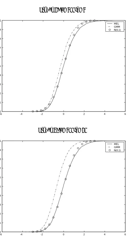
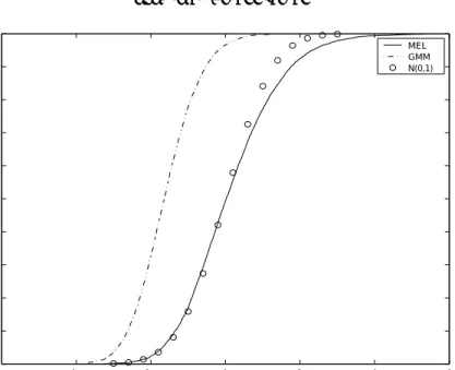
The most striking feature is that the distribution of the GMM estimator is skewed towards the left forα >0 (and towards the right forα <0), and the distortion increases withαand L .Figures 1, 2, and 3 show the estimated cdf’s of the MEL estimator and the GMM estimator for three representative cases among our many results. The MEL estimator is close to median-unbiased in each case while the GMM estimator is biased. As L increases, this bias becomes more serious; for L = 10 and L = 30 , the median is less than -1.0 ASD’s. IfL is large, the GMM estimator substantially underestimates the true parameter. The probability atx= 0 is about 1/2 +o(1/µ3) in (4.2) while it is 1/2 +αL/µ in (4.7), for instance. This fact definitely favors the MEL estimator over the GMM estimator. However, when L is as small as 3, the GMM estimator is very similar to the MEL and its distribution has tighter tails.
The distribution of the MEL estimator approaches normality faster than the dis-tribution of the GMM estimator, due primarily to the bias of the latter. In particular when α = 0 and L= 10,30,the actual 95 percentiles of the GMM estimator are sub-stantially different from 1.96 of the standard normal. This implies that the conventional hypothesis testing about a structural coefficient based on the normal approximation is very likely to seriously underestimate the actual significance. The 5 and 95 percentiles of the MEL estimator are much closer to those of the standard normal distribution even when Lis large.
4.3 Effects of Normality
Because the distributions of estimators depend on the distributions of the distur-bance terms, we have investigated the effects of non-normality of disturdistur-bances. Tables 7 and 8 are the distribution functions of the MEL and the GMM estimators when the disturbances follow the χ2 distribution and t(5) distribution, respectively. The former represents the skewed distribution while the latter represents the distributions with longer tails. From these tables the comparison of the distributions of the MEL and GMM estimators are approximately valid even if the distributions of disturbances are different from normal.
Also we have investigated the effects of exogenous variables on the distributions of estimators both in the cases when they are deterministic variables and non-normal stochastic variables. We have found that their effects are basically are negligible except some extreme situations and they are usually within the range of sampling variations of cdf estimates. This finding would be anticipated since the asymptotic expansions of the distributions are in the form of (4.2) and (4.7) under a set of assumptions. Hence we have omited to give the detailed discussions of these effects on our tables and figures.
5. Non-existence of Exact Moments of the MEL Estimator
As we have discussed in Section 4, we found that the finite sample distributions of the MEL estimator has considerable probabilities in their tail areas. This lead us to investigate the fundamental problem whether the MEL estimator does posses any moments of positive integer orders or not.
We first take a special case and consider the non-existence problem of moments. Let G1 = K = 1, K1 = 0, and we take z1i = 0,zi = zi∗ (i = 1,· · ·, n) . In this case, because of the boundedness condition that 0 < ≤ pˆi < 1 (i= 1,· · ·, n) and (2.11), we have the Lagrangian mltiplier λ(θ) = 0 with probability one. Then we have the estimated probabilities ˆpi = 1/n(i= 1,· · ·, n) and by using (2.9) the MEL estimator forβ becomes ˆ β = n i=1 z∗ iy1i n i=1 z∗iy2i . (5.1)
If we assume that (i) the seqence of random variables {y1i} and {y2i} are normally distributed, (ii) their distributions are not degenerated, and (iii) the sequence{zi∗} are strictly exogenous, then we can directly show that E[|βˆ|] = +∞ because ˆβ is a ratio of two normal random variables.
More generally, it is possible to show the non-existence of exact moments of the MEL estimator under a set of assumptions whenG1 ≥1.
Theorem 5.1 : In additon to the conditions in (2.18), (2.19), G1 ≥ 1 and n > K , assume the next conditions on the sequence of{zi} and {vi}.
[A1] The distributions of the sequences of random (vector) variables {vi} are abso-lutely continuous with respect to the Lebesgue measure and their densities are positive
everywhere inR1+G1 .
[A2] The sequence of{zi}are stochastic or non-stochastic vectors, which are indepen-dent of{vi},and theK×K moment matrix
Mn= 1 n n i=1 zizi (5.2)
is finite and positive definite with probability one. Then we have
E[|θˆi|] = +∞(i= 1,· · ·, p), (5.3)
where ˆθ= ( ˆθi) is the maximum empirical likelihood estimator ofθ .
Proof of Theorem 5.1 : First we use [A2] and (2.18). Since 0 < ≤ pi < 1 (i = 1,· · ·, n), we have the relation nMn < in=1pˆizizi < nMn with probability one. Then it is straightforward to show that
rank[ n i=1 ˆ pizizi] =K , rank[ n i=1 ˆ pizi( y2i z1i ) ] =p (5.4)
with probability one. By using (2.9) we haveK equations n i=1 ˆ piziy1i= n i=1 ˆ pizi(y2i,z1i)( ˆ β ˆ γ ). (5.5)
Because of [A1] we can take some p×1 vector sequence of variables {z∗i},which is a subset of vectorszi (i= 1,· · ·, n),such that
ˆ θ= [z∗1( y21 z11 ) + n i=2 liz∗i( y2i z1i ) ]−1[z∗1y11+ n i=2 liz∗iy1i], (5.6) whereli= ˆpi/pˆ1(i= 2,· · ·, n).
Without loss of generality we take anyp×1 (constant) vectorc1satisfying the conditions
c1 =0 and c1z1∗ = 0.Then we consider G1 equations with respect to the vectorsy∗21
and y∗2i(i= 2,· · ·, n) such that
y21∗ =− n i=2 c1z∗i c1z∗1liy ∗ 2i. (5.7)
Because li (i= 2,· · ·, n) are functions of y∗21 and they are bounded by the conditions onpi(i= 1,· · ·, n),there exists at least one solutiony21∗ satisfying the above equations given that the sequences y∗2i (i = 2,· · ·, n) and zi (i = 1,· · ·, n) are held fixed. (We can use the relations (2.7)-(2.12) for the linear case.) Also we notice that from [A1] the conditional density of theG1×1 random vectory21given y11 andy2i(i= 2,· · ·, n) is everywhere positive. Then for any real positive valueξ
P(c1z∗1y21+ n i=2 c1z∗iliy2i< ξ)>0 . (5.8)
This means that we have positive probabilities around the singular points of the inverse matrix on the right-hand side of (5.6). We notice that the determinant of the matrix
|z∗1( y21 z11 ) + n i=2 liz∗i( y2i z1i ) |
is a linear combination of each components of y21 and other random variables. Since
li(i= 2,· · ·, n) are bounded, the expected value of absolute value of each components in (5.6) with respect to the random variavlesy21 cannot be finite. Thus we have the desired result on the non-existence of moments. (Q.E.D.)
The non-existence of moments of the MEL estimator can explain its finite sample behaviors sometimes observed in Monte Carlo experiments. However, it should be important to note that the non-existence of exact moments do not necessarily mean that we should not use such estimation method. The classical simple example is the estimation problem of reciprocal of mean parameter in the i.i.d. univariate normal distribution, provided that it is not zero. The main issue is rather the choice of criteria for evaluating alternative estimation methods and we should be careful to use the bias and the mean squares error of estimators when they do not exist. Some related problems in the context of classical esonometric estimation methods were discussed by Anderson et. al. (1982).
In this paper we have discussed only the finite sample properties of alternative estimators for the unknown parameters. However, our result in this section has also an implication on the hypothesis testing problem. From our result it is likely that the statistics based on the empirical likelihood approach do not have any moments of positive integer orders. This problem has been previously pointed out by DiCiccio, Hall and Romano (1991) for a simple testing problem although their arguments are related but different from our arguments in this section.
6. Conclusions
First, the distributions of the MEL and GMM estimators are asymptotically equiv-alent in the sense of the limiting distribution, but their exact distributions are substan-tially different in finite samples. The MEL estimator is to be preferred to the GMM estimator if L is large. In the multiple equation cases and econometric models on panel data, for instance, it is often a common feature that L is fairly large. In such situations the MEL estimation method is particularly recommended.
Second, the large-sample normal approximation is relatively accurate for the MEL estimator. Hence the usual methods with asymptotic standard deviations gives reason-able inferences. On the other hand, for the GMM estimator the sample size should be very large to justify the use of procedures based on the normality when L is large, in particular.
Third, it would be recommendable to use the probability of concentration as a criterion of comparisons. It is because the MEL estimator does not posses any moments of positive integer orders and hence we expect to have some large absolute values of their bias and mean squares errors of estimators in the Monte Carlo simulations. In order to make fair comparisons of alternative estimators we need to use their culumative distribution functions and the concentration of probability.
To summarize the most important conclusion from the study of small sample dis-tributions of the MEL and GMM estimators is that the GMM estimator can be badly biased in some cases and in that sense its use is risky. The MEL estimator, on the other hand, has a little more variability with some chance of extreme values, but its distribution is centered at the true parameter value.
It is interesting that this conclusion is quite similar to the one on the comparative study of the LIML estimator over the TSLS (two-stage least squares) estimator in the same setting of linear structural equation, but with the restrictive assumption of the normal disturbances. ( See Section 5 of Anderson et. al. (1982).) This may be because that the maximum empirical likelihood (MEL) estimation of a structural equation can be interpreted as the semi-parametric analogue of the limited information maximum likelihood (LIML) estimation developed by Anderson and Rubin (1949) while the genaralized method of moments (GMM) estimation developed by Hansen (1982) can be interpreted as the semi-parametric analogue of the instrumental variables (IV) estimation developed by D.J. Sargan and H. Theil (see Sargan and Mikhail (1971), for instance) in the late 1950’s.
Finally there could be some ways to improve the small sample properties of the MEL estimation of structioral equations. Kunitomo (2002) and Kunitomo and Matsushita (2003) have already suggested one possible approach to this problem, which should be related to the issues investigated by Newey and Smith (2001). It should be an important topic because we have found that the distribution of the MEL estimator has fat-tails even in comparison with the LIML estimator in our study.
References
[1] Arellano, M. and B. Honor´e (2001) “Panel Data Models : Some Recent Devel-opments,” In Handbook of Econometrics, Vol. 5, edited by J. Heckman and E. Leamer.
[2] Anderson, T.W. (1974), “An Asymptotic Expansion of the Distribution of the Limited Information Maximum Likelihood Estimate of a Coefficient in a Simulta-neous Equation System,”Journal of the American Statistical Association, Vol. 69, 565-573.
[3] Anderson, T.W. and H. Rubin (1949), “Estimation of the Parameters of a Single Equation in a Complete System of Stochastic Equations,”Annals of Mathematical Statistics, Vol. 20, 46-63.
[4] Anderson, T.W. and T. Sawa (1973), “Distributions of Estimates of Coefficients of a Single Equation in a Simultaneous System and Their Asymptotic Expansion,”
Econometrica, Vol. 41, 683-714.
[5] Anderson, T.W. and T. Sawa (1979), “Evaluation of the Distribution Function of the Two-Stage Least Squares Estimate,” Econometrica, Vol. 47, 163-182.
[6] Anderson, T.W., N. Kunitomo, and T. Sawa (1982), “Evaluation of the Distribu-tion FuncDistribu-tion of the Limited InformaDistribu-tion Maximum Likelihood Estimator,” Econo-metrica, Vol. 50, 1009-1027.
[7] Anderson, T.W., N. Kunitomo, and K. Morimune (1986), “Comparing Single Equation Estimators in a Simultaneous Equation System,” Econometric Theory, Vol. 2, 1-32.
[8] DiCiccio, T., P. Hall, and J. Romano (1991), “Empirical Likelihood is Bartlett-Correctable,” The Annals of Statistics, Vol. 19-2, 1053-61.
[9] Fujikoshi, Y., K. Morimune, N. Kunitomo, and M. Taniguchi (1982), “Asymptotic Expansions of the Distributions of the Estimates of Coefficients in a Simultaneous Equation System,” Journal of Econometrics, Vol. 18, 2, 191-205.
[10] Hansen, L. (1982), “Large Sample Properties of Generalized Method of Moments Estimators,” Econometrica, Vol. 50, 1029-1054.
[11] Hayashi, F. (2000) Econometrics, Princeton University Press.
[12] Hsiao, C. (2003)Analysis of Panel Data, Cambridge University Press.
[13] Godambe, V.P. (1960), “An Optimum Property of Regular Maximum Likelihood Equation,” Annals of Mathematical Statistics, Vol. 31, 1208-1211.
[14] Kitamura, Y. (1997), “Empirical Likelihood Methods with Weakly Dependent Pro-cesses,” The Annals of Statistics, Vol.19-2, 1053-61.
[15] Kitamura, Y. G. Tripathi, and H. Ahn (2001), “Empirical Likelihood-Based Infer-ence in Conditional Moment Restriction Models,” Unpublished Manuscript.
[16] Kunitomo,N. (2002), “Improving Small Sample Properties of the Empirical Likeli-hood Estimator,” Discussion Paper CIRJE-F-184, Faculty of Economics, Univer-sity of Tokyo.
[17] Kunitomo,N. and Matsushita, Y. (2003), “Asymptotic Expansions of the Distri-butions of Semi-parametric Estimators in a Linear Simultaneous Equations Sys-tem,” Discussion Paper CIRJE-F-237, Faculty of Economics, University of Tokyo. (http://www.e.u-tokyo.ac.jp/cirje/research/dp/2003/2003cf237.pdf)
[18] Newey, W. K. and R. Smith (2001), “Higher Order Properties of GMM and Gen-eralized Empirical Likelihood Estimator,” Unpublished Manuscript.
[19] Owen, A. B. (1990), “Empirical Likelihood Ratio Confidence Regions,”The Annals of Statistics, Vol. 22, 300-325.
[20] Owen, A. B. (2001),Empirical Likelihood, Chapman and Hall.
[21] Phillips, P.C.B. (1980), “The Exact Finite Sample Density of Instrumental Vari-ables Estimators in an Equation with n+1 Endogenous VariVari-ables,” Econometrica, Vol. 48, 861-878.
[22] Phillips, P.C.B. (1983), “Exact Small Sample Theory in the Simultaneous Equa-tions Model,” Handbook of Econometrics, Vol. 1, 449-516, North-Holland.
[23] Qin, J. and Lawless, J. (1994), “Empirical Likelihood and General Estimating Equations,” The Annals of Statistics, Vol. 22, 300-325.
[24] Sargan, J. D. and Mikhail, W.M. (1971), “A General Approximation to the Dis-tribution of Instrumental Variables Estimates,”Econometrica, Vol. 39, 131-169.
APPENDIX : TABLES AND FIGURES Notes on Tables 1-8
In Tables 1-8 the distributions are tabulated in the standardized terms, that is, of (3.3). The tables include three quartiles, the 5 and 95 percentiles and the interquartile range of the distribution for each case. Since the limiting distributions of (3.3) areN(0,1) asn → ∞,we add the standard normal case as the bench mark.
Notes on Tables 9-10
In Tables 9 and 10 the cdf of two estimators and their differences are tabulated in the standardized terms, that is, of (3.3). The tables includes the three quartiles, the 2.5 and 97.5 percentiles and the interquartile range of the distribution for each case.
Notes on Figures
In Figures 1-3 the cdf of the MEL and GMM estimators are shown in the standardized terms, that is, of (3.3). The dotted line were used for the distributions of the GMM estimator. For the comparative purpose we give the standard normal distribution as the bench mark for each case.
Table 1: L= 3, α= 1
n= 100, L= 3, α= 1 n= 300, L= 3, α= 1
δ2= 50 δ2= 100 δ2= 50 δ2= 100
x normal MEL GMM MEL GMM MEL GMM MEL GMM
-3 0.001 0.000 0.000 0.000 0.000 0.000 0.000 0.000 0.000 -2.5 0.006 0.000 0.002 0.000 0.003 0.000 0.001 0.001 0.002 -2 0.023 0.013 0.023 0.014 0.022 0.009 0.016 0.012 0.019 -1.4 0.081 0.067 0.102 0.068 0.092 0.060 0.094 0.063 0.089 -1 0.159 0.146 0.209 0.145 0.191 0.143 0.212 0.141 0.192 -0.8 0.212 0.202 0.285 0.199 0.256 0.202 0.286 0.198 0.259 -0.6 0.274 0.268 0.368 0.261 0.330 0.271 0.369 0.266 0.337 -0.4 0.345 0.342 0.452 0.332 0.412 0.347 0.457 0.342 0.424 -0.2 0.421 0.420 0.533 0.411 0.493 0.429 0.542 0.422 0.508 0 0.500 0.498 0.612 0.491 0.572 0.506 0.624 0.506 0.587 0.2 0.579 0.571 0.686 0.567 0.647 0.581 0.702 0.587 0.664 0.4 0.655 0.641 0.753 0.638 0.715 0.654 0.766 0.657 0.729 0.6 0.726 0.705 0.806 0.703 0.774 0.719 0.818 0.717 0.786 0.8 0.788 0.761 0.847 0.762 0.824 0.773 0.861 0.771 0.833 1 0.841 0.808 0.883 0.811 0.868 0.818 0.895 0.820 0.873 1.4 0.919 0.880 0.937 0.887 0.928 0.888 0.944 0.895 0.933 2 0.977 0.945 0.977 0.950 0.973 0.950 0.980 0.960 0.975 2.5 0.994 0.971 0.991 0.977 0.987 0.977 0.992 0.981 0.990 3 0.999 0.987 0.996 0.988 0.995 0.989 0.996 0.992 0.997 X05 -1.65 -1.53 -1.73 -1.54 -1.68 -1.47 -1.65 -1.49 -1.64 L.QT -0.67 -0.65 -0.89 -0.63 -0.82 -0.66 -0.90 -0.64 -0.83 MEDN 0.00 0.01 -0.28 0.02 -0.18 -0.02 -0.30 -0.01 -0.22 U.QT 0.67 0.76 0.39 0.76 0.52 0.71 0.35 0.72 0.47 X95 1.65 2.08 1.55 2.00 1.63 2.00 1.47 1.86 1.57 IQR 1.35 1.41 1.28 1.39 1.33 1.37 1.24 1.36 1.30 19
Table 2: L= 10, α= 1
n= 100, L= 10, α= 1 n= 300, L= 10, α= 1
δ2= 50 δ2= 100 δ2= 50 δ2= 100
x normal MEL GMM MEL GMM MEL GMM MEL GMM
-3 0.001 0.001 0.004 0.000 0.002 0.000 0.000 0.000 0.002 -2.5 0.006 0.006 0.021 0.004 0.014 0.001 0.012 0.003 0.014 -2 0.023 0.023 0.082 0.017 0.055 0.015 0.070 0.018 0.055 -1.4 0.081 0.093 0.264 0.086 0.196 0.076 0.249 0.074 0.201 -1 0.159 0.186 0.432 0.165 0.350 0.160 0.429 0.158 0.359 -0.8 0.212 0.244 0.519 0.221 0.433 0.217 0.520 0.219 0.447 -0.6 0.274 0.308 0.609 0.286 0.517 0.283 0.610 0.286 0.536 -0.4 0.345 0.377 0.689 0.354 0.601 0.355 0.693 0.357 0.622 -0.2 0.421 0.445 0.762 0.429 0.675 0.430 0.769 0.434 0.700 0 0.500 0.510 0.822 0.506 0.738 0.503 0.830 0.514 0.764 0.2 0.579 0.576 0.871 0.574 0.796 0.574 0.877 0.588 0.821 0.4 0.655 0.639 0.909 0.636 0.845 0.640 0.912 0.655 0.868 0.6 0.726 0.696 0.936 0.695 0.882 0.703 0.939 0.718 0.904 0.8 0.788 0.748 0.957 0.747 0.914 0.758 0.960 0.772 0.931 1 0.841 0.792 0.971 0.792 0.938 0.802 0.974 0.819 0.950 1.4 0.919 0.860 0.986 0.865 0.968 0.874 0.989 0.889 0.977 2 0.977 0.924 0.997 0.934 0.990 0.935 0.997 0.952 0.994 2.5 0.994 0.952 0.999 0.964 0.997 0.961 0.999 0.977 0.999 3 0.999 0.970 1.000 0.981 0.999 0.977 1.000 0.991 1.000 X05 -1.65 -1.70 -2.19 -1.63 -2.04 -1.58 -2.11 -1.60 -2.04 L.QT -0.67 -0.78 -1.44 -0.71 -1.25 -0.70 -1.40 -0.70 -1.26 MEDN 0 -0.03 -0.84 -0.02 -0.64 -0.01 -0.84 -0.04 -0.68 U.QT 0.67 0.81 -0.23 0.81 0.04 0.77 -0.25 0.71 -0.05 X95 1.65 2.46 0.73 2.24 1.14 2.25 0.70 1.97 1.00 IQR 1.35 1.59 1.20 1.52 1.28 1.47 1.15 1.42 1.22 20
Table 3: L= 20,30, α= 1
n= 100, L= 20, α= 1 n= 300, L= 30, α= 1
δ2 = 100 δ2= 300 δ2= 100 δ2= 300
x normal MEL GMM MEL GMM MEL GMM MEL GMM
-3 0.001 0.008 0.018 0.006 0.011 0.001 0.036 0.002 0.018 -2.5 0.006 0.021 0.066 0.019 0.038 0.006 0.133 0.008 0.061 -2 0.023 0.053 0.177 0.049 0.101 0.023 0.327 0.029 0.164 -1.4 0.081 0.138 0.407 0.126 0.262 0.091 0.616 0.093 0.383 -1 0.159 0.224 0.582 0.207 0.407 0.173 0.777 0.174 0.549 -0.8 0.212 0.273 0.666 0.257 0.486 0.231 0.837 0.225 0.632 -0.6 0.274 0.327 0.739 0.312 0.568 0.294 0.885 0.285 0.707 -0.4 0.345 0.387 0.803 0.374 0.644 0.360 0.922 0.356 0.769 -0.2 0.421 0.448 0.853 0.438 0.713 0.428 0.949 0.431 0.823 0 0.500 0.508 0.892 0.502 0.777 0.493 0.966 0.504 0.866 0.2 0.579 0.567 0.924 0.564 0.830 0.556 0.978 0.572 0.901 0.4 0.655 0.622 0.949 0.624 0.871 0.617 0.986 0.641 0.929 0.6 0.726 0.675 0.967 0.680 0.902 0.674 0.992 0.705 0.951 0.8 0.788 0.726 0.979 0.729 0.928 0.726 0.996 0.761 0.967 1 0.841 0.770 0.987 0.775 0.948 0.772 0.998 0.808 0.979 1.4 0.919 0.839 0.995 0.851 0.978 0.847 1.000 0.876 0.991 2 0.977 0.910 0.999 0.929 0.995 0.925 1.000 0.944 0.998 2.5 0.994 0.945 1.000 0.964 0.998 0.959 1.000 0.974 1.000 3 0.999 0.968 1.000 0.981 0.999 0.978 1.000 0.990 1.000 X05 -1.65 -2.03 -2.62 -1.99 -2.37 -1.69 -2.89 -1.73 -2.59 L.QT -0.67 -0.89 -1.79 -0.82 -1.44 -0.74 -2.17 -0.71 -1.74 MEDN 0 -0.03 -1.19 -0.01 -0.77 0.02 -1.64 -0.01 -1.12 U.QT 0.67 0.91 -0.57 0.89 -0.09 0.90 -1.08 0.76 -0.46 X95 1.65 2.59 0.41 2.25 1.02 2.33 -0.19 2.08 0.59 IQR 1.35 1.80 1.22 1.71 1.35 1.64 1.09 1.47 1.27 21
Table 4: α= 0
n= 100, L= 3 n= 100, L= 20 n= 300, L= 10 n= 300, L= 30
α= 0, δ2= 30 α= 0, δ2= 100 α= 0, δ2= 50 α= 0, δ2= 100
x normal MEL GMM MEL GMM MEL GMM MEL GMM
-3 0.001 0.009 0.003 0.022 0.002 0.011 0.001 0.018 0.003 -2.5 0.006 0.021 0.009 0.045 0.008 0.022 0.006 0.036 0.007 -2 0.023 0.049 0.028 0.084 0.025 0.050 0.020 0.068 0.019 -1.4 0.081 0.117 0.089 0.161 0.082 0.119 0.071 0.145 0.068 -1 0.159 0.191 0.161 0.233 0.157 0.202 0.151 0.220 0.139 -0.8 0.212 0.243 0.216 0.274 0.211 0.254 0.206 0.268 0.191 -0.6 0.274 0.300 0.281 0.324 0.274 0.310 0.270 0.321 0.255 -0.4 0.345 0.367 0.353 0.377 0.345 0.368 0.339 0.380 0.333 -0.2 0.421 0.438 0.431 0.433 0.421 0.432 0.415 0.442 0.416 0 0.500 0.511 0.512 0.492 0.499 0.502 0.501 0.504 0.501 0.2 0.579 0.583 0.590 0.550 0.575 0.574 0.584 0.564 0.582 0.4 0.655 0.651 0.662 0.604 0.649 0.639 0.662 0.619 0.662 0.6 0.726 0.712 0.731 0.656 0.719 0.698 0.733 0.671 0.737 0.8 0.788 0.766 0.792 0.706 0.781 0.753 0.799 0.724 0.801 1 0.841 0.815 0.842 0.756 0.835 0.801 0.852 0.772 0.858 1.4 0.919 0.895 0.920 0.835 0.918 0.881 0.927 0.852 0.932 2 0.977 0.962 0.979 0.915 0.974 0.951 0.981 0.932 0.982 2.5 0.994 0.983 0.992 0.956 0.993 0.979 0.996 0.965 0.995 3 0.999 0.990 0.997 0.976 0.998 0.990 1.000 0.984 0.999 X05 -1.65 -1.99 -1.73 -2.43 -1.67 -1.99 -1.56 -2.24 -1.54 L.QT -0.67 -0.77 -0.69 -0.91 -0.67 -0.82 -0.66 -0.87 -0.61 MEDN 0 -0.03 -0.03 0.03 0.00 -0.01 0.00 -0.01 0.00 U.QT 0.67 0.74 0.66 0.98 0.70 0.79 0.65 0.90 0.64 X95 1.65 1.85 1.64 2.40 1.68 1.98 1.59 2.23 1.55 IQR 1.35 1.51 1.35 1.89 1.37 1.61 1.31 1.77 1.25 22
Table 5: α= 5
n= 100, L= 3 n= 100, L= 20 n= 300, L= 10 n= 300, L= 30
α= 5, δ2= 50 α= 5, δ2= 100 α= 5, δ2= 50 α= 5, δ2= 100
x normal MEL GMM MEL GMM MEL GMM MEL GMM
-3 0.001 0.000 0.000 0.001 0.031 0.000 0.000 0.000 0.124 -2.5 0.006 0.000 0.000 0.008 0.131 0.000 0.016 0.001 0.356 -2 0.023 0.004 0.014 0.029 0.326 0.004 0.098 0.013 0.634 -1.4 0.081 0.046 0.099 0.101 0.625 0.045 0.362 0.070 0.873 -1 0.159 0.129 0.231 0.185 0.781 0.127 0.588 0.155 0.948 -0.8 0.212 0.189 0.315 0.240 0.838 0.187 0.685 0.212 0.967 -0.6 0.274 0.260 0.406 0.305 0.885 0.258 0.761 0.274 0.980 -0.4 0.345 0.340 0.492 0.375 0.921 0.337 0.822 0.344 0.988 -0.2 0.421 0.415 0.573 0.444 0.946 0.415 0.873 0.420 0.993 0 0.500 0.492 0.654 0.508 0.965 0.493 0.912 0.498 0.996 0.2 0.579 0.570 0.725 0.568 0.978 0.571 0.939 0.575 0.998 0.4 0.655 0.638 0.780 0.628 0.986 0.643 0.957 0.639 1.000 0.6 0.726 0.697 0.824 0.681 0.991 0.701 0.971 0.697 1.000 0.8 0.788 0.749 0.862 0.728 0.994 0.754 0.981 0.752 1.000 1 0.841 0.798 0.894 0.772 0.996 0.801 0.988 0.799 1.000 1.4 0.919 0.872 0.939 0.850 0.998 0.875 0.996 0.870 1.000 2 0.977 0.939 0.976 0.917 1.000 0.937 0.999 0.935 1.000 2.5 0.994 0.968 0.988 0.951 1.000 0.962 1.000 0.966 1.000 3 0.999 0.981 0.994 0.970 1.000 0.978 1.000 0.983 1.000 X05 -1.65 -1.37 -1.64 -1.77 -2.86 -1.37 -2.22 -1.55 -3.31 L.QT -0.67 -0.63 -0.95 -0.77 -2.17 -0.62 -1.61 -0.68 -2.70 MEDN 0 0.02 -0.38 -0.03 -1.66 0.02 -1.16 0.00 -2.25 U.QT 0.67 0.80 0.29 0.90 -1.10 0.79 -0.63 0.79 -1.76 X95 1.65 2.14 1.54 2.48 -0.17 2.23 0.32 2.21 -0.98 IQR 1.35 1.43 1.24 1.67 1.07 1.41 0.98 1.47 0.95 23
Table 6: n= 50
n= 50, L= 3 n= 50, L= 3 n= 50, L= 10 n= 50, L= 10
α= 1, δ2= 50 α= 5, δ2= 50 α = 1, δ2= 100 α = 5, δ2= 100
x normal MEL GMM MEL GMM MEL GMM MEL GMM
-3 0.001 0.000 0.000 0.000 0.000 0.005 0.004 0.001 0.004 -2.5 0.006 0.001 0.002 0.000 0.000 0.016 0.016 0.008 0.023 -2 0.023 0.012 0.020 0.004 0.014 0.042 0.064 0.028 0.088 -1.4 0.081 0.069 0.101 0.047 0.105 0.120 0.216 0.098 0.277 -1 0.159 0.153 0.214 0.132 0.239 0.205 0.365 0.183 0.448 -0.8 0.212 0.205 0.285 0.191 0.322 0.260 0.448 0.239 0.538 -0.6 0.274 0.271 0.368 0.260 0.413 0.326 0.534 0.302 0.624 -0.4 0.345 0.346 0.452 0.338 0.499 0.394 0.614 0.366 0.697 -0.2 0.421 0.424 0.536 0.418 0.582 0.461 0.682 0.438 0.761 0 0.500 0.502 0.615 0.496 0.656 0.526 0.743 0.511 0.816 0.2 0.579 0.575 0.683 0.572 0.719 0.589 0.801 0.575 0.859 0.4 0.655 0.640 0.746 0.640 0.777 0.649 0.850 0.635 0.893 0.6 0.726 0.701 0.803 0.700 0.826 0.702 0.886 0.685 0.920 0.8 0.788 0.758 0.851 0.756 0.864 0.748 0.914 0.732 0.941 1 0.841 0.806 0.886 0.803 0.893 0.788 0.937 0.774 0.958 1.4 0.919 0.878 0.935 0.868 0.938 0.852 0.968 0.843 0.978 2 0.977 0.942 0.975 0.934 0.976 0.918 0.990 0.913 0.992 2.5 0.994 0.968 0.990 0.961 0.988 0.951 0.997 0.948 0.997 3 0.999 0.981 0.995 0.977 0.995 0.972 0.999 0.969 0.999 X05 -1.65 -1.53 -1.70 -1.38 -1.66 -1.91 -2.09 -1.73 -2.23 L.QT -0.67 -0.66 -0.89 -0.63 -0.97 -0.83 -1.30 -0.76 -1.47 MEDN 0 0.00 -0.29 0.01 -0.40 -0.08 -0.68 -0.03 -0.88 U.QT 0.67 0.77 0.41 0.78 0.31 0.81 0.02 0.88 -0.24 X95 1.65 2.13 1.57 2.25 1.54 2.48 1.15 2.53 0.90 IQR 1.35 1.43 1.31 1.40 1.28 1.64 1.33 1.65 1.23 24
Table 7: χ2(3) case
n= 100, L= 3 n= 100, L= 20 n= 300, L= 10
α= 1, δ2 = 50 α= 1, δ2= 100 α= 1, δ2 = 50
x normal MEL GMM MEL GMM MEL GMM
-3 0.001 0.000 0.000 0.004 0.008 0.001 0.001 -2.5 0.006 0.000 0.001 0.011 0.039 0.004 0.011 -2 0.023 0.008 0.013 0.031 0.123 0.013 0.050 -1.4 0.081 0.057 0.083 0.098 0.337 0.068 0.211 -1 0.159 0.134 0.189 0.184 0.522 0.151 0.391 -0.8 0.212 0.194 0.264 0.236 0.617 0.209 0.488 -0.6 0.274 0.261 0.347 0.296 0.696 0.275 0.584 -0.4 0.345 0.338 0.436 0.360 0.769 0.349 0.676 -0.2 0.421 0.420 0.523 0.428 0.831 0.423 0.762 0 0.500 0.499 0.605 0.498 0.879 0.497 0.828 0.2 0.579 0.572 0.681 0.566 0.914 0.570 0.877 0.4 0.655 0.640 0.746 0.632 0.940 0.644 0.915 0.6 0.726 0.702 0.800 0.691 0.959 0.706 0.943 0.8 0.788 0.758 0.848 0.743 0.972 0.757 0.962 1 0.841 0.808 0.889 0.790 0.982 0.803 0.975 1.4 0.919 0.881 0.940 0.862 0.994 0.876 0.991 2 0.977 0.945 0.976 0.931 1.000 0.942 0.998 2.5 0.994 0.969 0.989 0.965 1.000 0.971 0.999 3 0.999 0.982 0.995 0.982 1.000 0.983 0.999 X05 -1.65 -1.46 -1.60 -1.77 -2.40 -1.52 -2.00 L.QT -0.67 -0.63 -0.84 -0.75 -1.60 -0.67 -1.30 MEDN 0 0.00 -0.25 0.01 -1.04 0.01 -0.78 U.QT 0.67 0.77 0.42 0.83 -0.46 0.77 -0.23 X95 1.65 2.10 1.52 2.26 0.50 2.10 0.66 IQR 1.35 1.40 1.25 1.58 1.15 1.44 1.07 25
Table 8: t(5) case
n= 100, L= 3 n= 100, L= 20 n= 300, L= 10
α= 1, δ2 = 50 α= 1, δ2= 100 α= 1, δ2 = 50
x normal MEL GMM MEL GMM MEL GMM
-3 0.001 0.000 0.000 0.004 0.010 0.000 0.000 -2.5 0.006 0.002 0.003 0.012 0.042 0.001 0.013 -2 0.023 0.012 0.018 0.037 0.144 0.012 0.065 -1.4 0.081 0.055 0.089 0.108 0.385 0.063 0.253 -1 0.159 0.136 0.208 0.199 0.576 0.148 0.444 -0.8 0.212 0.193 0.287 0.251 0.664 0.205 0.543 -0.6 0.274 0.266 0.372 0.307 0.747 0.271 0.638 -0.4 0.345 0.347 0.459 0.371 0.813 0.347 0.721 -0.2 0.421 0.428 0.550 0.439 0.863 0.427 0.791 0 0.500 0.510 0.634 0.511 0.904 0.505 0.848 0.2 0.579 0.586 0.705 0.580 0.936 0.579 0.890 0.4 0.655 0.655 0.767 0.642 0.959 0.646 0.921 0.6 0.726 0.715 0.818 0.698 0.974 0.702 0.945 0.8 0.788 0.769 0.862 0.748 0.983 0.754 0.964 1 0.841 0.816 0.897 0.794 0.990 0.800 0.977 1.4 0.919 0.885 0.945 0.861 0.997 0.871 0.990 2 0.977 0.944 0.979 0.928 1.000 0.935 0.996 2.5 0.994 0.971 0.991 0.957 1.000 0.965 0.998 3 0.999 0.983 0.996 0.976 1.000 0.978 1.000 X05 -1.65 -1.44 -1.61 -1.84 -2.44 -1.50 -2.09 L.QT -0.67 -0.64 -0.89 -0.80 -1.69 -0.66 -1.41 MEDN 0 -0.02 -0.31 -0.03 -1.17 -0.01 -0.89 U.QT 0.67 0.73 0.34 0.81 -0.59 0.79 -0.32 X95 1.65 2.09 1.46 2.37 0.31 2.20 0.65 IQR 1.35 1.37 1.23 1.61 1.10 1.44 1.09 26
Table 9: Accuracy of the cdf of GMM (1)
n= 100, L= 2, α= 1
δ2 = 50 δ2 = 100
x Exact Our Method Difference Exact Our Method Difference -3.0 0.000 0.000 0.000 0.000 0.000 0.000 -2.5 0.001 0.001 0.000 0.002 0.001 -0.001 -2.0 0.012 0.012 0.000 0.015 0.016 0.001 -1.5 0.061 0.054 -0.007 0.063 0.064 0.001 -1 0.181 0.178 -0.004 0.175 0.181 0.006 -0.8 0.251 0.250 -0.001 0.239 0.246 0.007 -0.6 0.331 0.332 0.001 0.313 0.316 0.003 -0.4 0.414 0.417 0.003 0.393 0.395 0.002 -0.2 0.498 0.503 0.005 0.476 0.480 0.004 0 0.580 0.587 0.007 0.557 0.565 0.008 0.2 0.655 0.661 0.006 0.633 0.641 0.008 0.5 0.752 0.752 0.000 0.735 0.741 0.006 1.0 0.868 0.870 0.002 0.860 0.857 -0.003 2.0 0.969 0.971 0.002 0.971 0.971 0.000 3.0 0.993 0.992 -0.001 0.995 0.995 0.000 X025 -1.80 -1.78 0.02 -1.84 -1.86 -0.02 L.QT -0.80 -0.80 0.00 -0.77 -0.79 -0.02 MEDN -0.20 -0.21 -0.01 -0.14 -0.15 -0.01 U.QT 0.49 0.49 0.00 0.55 0.53 -0.02 X975 2.14 2.12 -0.02 2.09 2.09 0.00 IQR 1.29 1.29 0.00 1.32 1.32 0.00 27
Table 10: Accuracy of the cdf of GMM (2)
n= 300, L= 29
α= 1, δ2= 100 α= 5, δ2= 100
x Exact Our Method Difference Exact Our Method Difference -3.0 0.024 0.024 0.000 0.090 0.095 0.005 -2.5 0.108 0.108 0.000 0.322 0.327 0.005 -2.0 0.295 0.290 -0.005 0.630 0.631 0.001 -1.5 0.551 0.545 -0.006 0.852 0.855 0.003 -1.0 0.776 0.772 -0.004 0.954 0.955 0.001 -0.8 0.841 0.841 0.000 0.973 0.974 0.001 -0.6 0.892 0.894 0.002 0.985 0.985 0.000 -0.4 0.929 0.931 0.002 0.991 0.991 0.000 -0.2 0.955 0.956 0.001 0.995 0.996 0.001 0 0.972 0.972 0.000 0.997 0.998 0.001 0.2 0.983 0.982 -0.001 0.999 1.000 0.001 0.5 0.992 0.992 0.000 1.000 1.000 0.000 1.0 0.998 0.999 0.001 1.000 1.000 0.000 2.0 1.000 1.000 0.000 1.000 1.000 0.000 3.0 1.000 1.000 0.000 1.000 1.000 0.000 X025 -2.99 -2.99 0.00 -3.32 -3.31 0.01 L.QT -2.10 -2.09 0.01 -2.63 -2.64 -0.01 MEDN -1.60 -1.59 0.01 -2.22 -2.22 0.00 U.QT -1.07 -1.06 0.01 -1.77 -1.77 0.00 X0975 0.05 0.05 0.01 -0.78 -0.78 -0.01 IQR 1.03 1.04 0.00 0.86 0.87 0.01 28
Figure 1: n=300,L=3 -6 -4 -2 0 2 4 6 0 0.1 0.2 0.3 0.4 0.5 0.6 0.7 0.8 0.9 1 MEL GMM N(0,1) Figure 2: n=300,L=10 -6 -4 -2 0 2 4 6 0 0.1 0.2 0.3 0.4 0.5 0.6 0.7 0.8 0.9 1 MEL GMM N(0,1) 29
Figure 3: n=300,L=30 -6 -4 -2 0 2 4 6 0 0.1 0.2 0.3 0.4 0.5 0.6 0.7 0.8 0.9 1 MEL GMM N(0,1) 30