Bayesian Variable Selection of Risk Factors in the APT Model

School of Economics

UNSW, Sydney 2052

Australia

http://www.economics.unsw.edu.au

The views expressed in this paper are those of the authors and do not necessarily reflect those of the School of Economic at UNSW.

Bayesian Variable Selection of Risk factors in the

APT Model

Robert Kohn and Rachida Ouysse

Robert Kohn

_{Rachida Ouysse}

October 29, 2007

Abstract

In this paper we use a probabilistic approach to risk factor selection in the arbitrage pricing theory model. The methodology uses a bayesian framework to simultaneously select the perva-sive risk factors and estimate the model. This will enable correct inference and testing of the implications of the APT model. Furthermore, we are able to make inference on any function of the parameters, in particular the pricing errors. We can also carry out tests of efficiency of the APT using the posterior odds ratio and bayesian confidence intervals. We investigate the macroeconomic risk factors of Chen, Roll, and Ross (1986) and the firm characteristic factors of Fama and French (1992,1993). Using monthly portfolio returns grouped by size and book to market, we find that the economic variables have zero risk premia although some appear to have non zero posterior probability. The ”Market” factor is not priced. An APT model with factors mimicking size (SMB), book to market equity (HML), value-weighted portfolio and Standard and Poor, is supported by a conditionally independent prior and offers a significant decrease in the pricing error over a two-factor APT with SMB and HML. The posterior probability and cumula-tive distributions functions of the average risk premia and the pricing errors are compared to the normal distribution. The results show that under certain conditions the distortions are very small.

JEL Classification: C1, C22, C52

Keywords: Variable selection, Posterior density, Bayes factors, MCMC, APT models.

∗_{School of Economics, The University Of New South Wales, Sydney 2052 Australia. Email: [email protected]} †_{School of Economics, The University Of New South Wales, Sydney 2052 Australia. Email: [email protected]}

1

Introduction

In this paper, we address model selection in the context of a linear factor model with potentially measured and latent factors. The study proposes an exact statistical framework for the estimation and inference in a factor model. We use a bayesian framework to implicitly incorporate model uncertainty into the estimation of the parameters and model inference.

Since the inception of the arbitrage pricing theory (APT) by Ross (1976, 1977), there is an increased interest in the use of linear factor models in the study of Asset pricing. There is a growing evidence that high returns are driven by a multi-factor model rather than the one factor capital pricing model (CAPM)1_{. The APT has the attractive feature of minimal assumptions about the nature of the}

economy. However, this tractability comes at the cost of certain ambiguities such as an approximate pricing relation and an unknown set of pervasive factors. In order to test the implications of the APT, one must specify the number and the identity of the factors.

There are two main streams in the literature of factor selection in the APT. The first view toward model determination uses latent (unobservable) factors as sources of common variations. These common factors are estimated from sample covariance matrices using statistical techniques like factor analysis and principal components. Bai and Ng (2000) develops an econometric approach to consistently determine the dimension of the model for large panels. Bai (2001) addresses the asymptotic properties of the estimated model. This literature addresses the asymptotic properties of the distributions and therefore is based on the model selection being consistent and therefore treated as deterministic. The second alternative view suggests the use of observed economic variables as factors. There is no doubt that asset prices are intimately linked to macroeconomic activity and that the influences go in both directions. However, little is done to formalize the search for the set of significant influential variables. Chen, Roll and Ross (1986) (CRR) asserts “A rather embarrassing gap exists between the theoretically exclusive importance of systematic “state variables” and our complete ignorance of their identity”. CRR attempts to explore this identification terrain by combining a set of “likely” macroe-conomic and financial candidates for pervasive risk in asset returns. The selection procedure consists of a series of t-test for the significance of average risk premia corresponding to each of the variables allowed into the regression. The authors identify five common risk factors that are significantly priced in the stock market. Using a different approach, based on firm characteristics as a proxy for the firms’ sensitivity to systematic risk in the economy, Fama and French (1993) shows that the variation in returns on stocks and bonds can be explained by five size and book-to-market based factors. How-ever, these studies raise two fundamental critiques. First, the number of factors is often assumed and arbitrarily prespecified. Second, the set of potential pervasive factors is subjectively reduced to a few number of candidates and only a few specifications are tested. Hence, no statistical justification is provided to justify the selected set of variables. Ouysse (2006) proposes a formal econometric proce-dure to consistently select the set of pervasive factors in panels with large dimensions. However, the study does not address the post-selection properties of the model estimates.

The APT implies nonlinear restrictions on the model parameters, which make it very difficult and complex to derive the asymptotic distribution of the restricted estimates, let alone, the distribution of post-selection restricted estimates. The bayesian approach enables exact inference by making it possible to implicitly incorporate model uncertainty and to derive post-selection distributions of any functions of the parameters.

Geweke and Zhou (1996) uses a bayesian framework to analyze the APT. The authors propose the use of the pricing error to test the implication the APT that the expected returns are approximately linear function of the risk premium on systematic factors. The authors use latent factors and do not perform a selection of the appropriate number of factors. They borrow the results from the asymptotic principal component analysis of Connor and Korajczyk (1986,1993) and propose the use of 1 to 4 factors.

The present study extends [[16]] to allow for both latent and measured factors. In particular, this method makes it possible to derive the exact post-selection posterior distributions for the measures of the pricing error and for the measure of the systematic risk and risk premia.

1_{For example, Fama and French (1996) indicates that market anomalies largely disappear in a three-factor model.}

2

Methodology

2.1

Asset Pricing model

In the finance literature, the debate on what drives excess returns continues. A large number of studies use factor models to identify the common sources of systematic risk in expected returns. The factors used are classified into latent factors estimated through statistical methods as principal components and factor analysis and observable factors based on the sensitivity of stocks returns to economic and financial news. The use of observable variables to explain excess returns is particularly appealing. The estimated factor loadings have a meaningful interpretation. The estimated pricing relationship can be used to stimulate the financial markets through the pervasive economic and financial variables. The ability to predict excess returns with tangible factors can be useful for portfolio management and stock market investment decisions.

Unlike the Capital Asset Pricing model, theAP T allows for multiple risk factors to enter the return generating process for asset returns. In a rational asset pricing model with multiple beta, expected returns of securities are related to their sensitivities to changes in the state of the economy.

LetYitbe the return on assetiat timet. Assume that asset returns follow an approximate2k0−factor

model3_, Yit=αi+ k0 X j=2 bijxtj+εti (1)

The interceptαiis the expected return on asseti, αi=E[Yit].The risk factors are common across the

assets. Therefore, the asset risk can be divided into a common diversifiable risk due to the exposure to thek0 common risk factorsxt,and an idiosyncratic non-diversifiable risk due to the idiosyncratic

factor εit. The betas bij, or factor loadings of the jth factor for asset i, represent the amount of

exposure to each risk factor. There areT time periods andN assets.

In our analysis, it is convenient to work with the pooled form of the model. Lety=vec(Y),β=vec(B),

andε=vec(v), y N T×1= (IN TN⊗×N kX) β N k×1 + ε N T×1 (2)

The idiosyncratic factors are assumed to be uncorrelated with the factors,X.They are also assumed to have a normal distribution with mean zero and covariance matrix Σ⊗IT4.

The absence of riskless arbitrage opportunities implies well-known restrictions on (1), namely

αi ≈ δ0+βi1δ1+...+βik0δk0 (3)

i = 1, .., N

where λ15 is the riskless return, provided at least one risk-averse investor holds a portfolio without

any residual risk andλj is the risk premium onjthfactor. Equation (3) represents an approximate6

linear relationship between the expected asset returns and their risk exposures.It implies that the risk premium on an asset, (βi2λ2+...+βik0λk0),by its factor loadings. Exact arbitrage pricing obtains

when (3) holds with equality.

Geweke and Zhou (1996) proposes a measure of pricing error given by the average of squared deviations from the restriction across assets. The pricing error is measured by

Q2 N = N X i=1 (αi−δ0−βi1δ1−...−βik0δk0) 2 /N QN → 0 asN → ∞

2_{An approximate factor structure, first introduced by Chamberlain and Rothschild (1983), relaxes the static factor}

model assumption of diagonal idiosyncratic covariance matrix to allow for a limited amount of cross-section dependence.

3_{The APT is based on the pricing relation for a countably infinite vector of returns to a countably infinite set of}

traded assets.

4_{If there is serial correlation, the covariance matrix will be of the more general form,E(εε}0_{) = Σ⊗Γ.}

5_{The riskless rate will be measured by the 30-day Treasury-bill rate that is known at the beginning of each period}

month.

The authors argue that for Connor’s equilibrium APT, Q is equal to zero. For Ross’s asymptotic APT, the pricing error will converge to zero as the number of assets approaches infinity. Although for fixedN, the pricing error is not necessarily small, the authors suggest the use of the pricing error to examine some of the testable implications of the APT.

Another measure of the pricing error which takes into account the cross section correlation structure in the idiosyncratic term is given by,

e Q2 N = ³ α−Be0_δ´0_Ω³_α−Be0_δ´ N e B = (ı, B); δ= (δ0, ..., δk0) 0 e QN → 0 asN → ∞

Stated differently, the pricing theory imposes a testable cross-equation restriction on the parameters of a multivariate regression of asset excess returns on the factors7_{It implies zero intercepts in a regression}

of asset excess returns on the factors. A test of miss-pricing is a test for non-zero intercept.

2.2

Review of the Classical Inference

There are mainly two approaches to estimating and testing the APT. First, traditional factor analysis uses a likelihood ratio to test the restrictions implied by the APT. This involves computing the maximum likelihood estimates under the nonlinear restrictions in (3.) This is a very difficult task in practice and the model inference is non standard. Indeed, [1] shows that the asymptotic distributions of the model parameters estimates are very complex in factor analysis, and the constrained estimates should be even more complex. This complexity makes it difficult to derive the asymptotic distribution of the likelihood ratio tests.

The second approaches surmount the complexity of the estimation under nonlinear restrictions by a two-pass approach. In the first pass, either the factor loading or the factors are estimated. In order to estimate the factors betas (factor loading) of assets, excess returns are regressed against the common factors using the time series from t−60 to t−1 to get the conditional betasβbik,t−1.The estimates

n b

βik

ok=1,..,K

i=1,..,N are then used in the second pass.

Treating these estimates as the true variables, the APT restrictions in (3) become linear constraints on the coefficients of the multivariate regression. In fact, these restrictions imply zero intercepts and can be tested using the standard methods. To estimate the risk premia, a cross sectional regression model is utilized for each time point to get the time series of each risk premia. For each monthtof the next 12 months, perform cross section regressions: Yit=δ0t+

PK

k=1βik,t−1δkt+εit withi= 1, .., N

and get an estimate of the sum of risk premiumδbkt for monthtassociated to variablek, t= 1, ..,12.

The two-pass steps are repeated for each time period in the sample.

Estimation technique: (i) Regress excess returns on the economic variables using the time series from

t−60 tot−1 to get the conditional betasβbik,t−1. (ii) For each monthtof the next 12 months, perform

cross section regressions: Rit=δ0t+

PK

k=1βik,t−1δkt+εitwithi= 1, .., N and get an estimate of the

sum of risk premiumδbkt for month t associated to variable k, t= 1, ..,12. (iii) Steps (i) and (ii) are

repeated for each year in the sample period. The time series means of the series of of risk premium

7_{The equilibrium version of the APT implies that}

E(yt) =rF te+Bλe t (4)

where rF t represents the return on a riskless asset,eis a vector of ones,λt is ak0−vector of factor risk premiums.

Combining equations (??) and (4) gives,

e

Y =BeXe+v

where theN×T matrix of excess returns is given byYe =Y −IN r0F andXe is theT ×k0 realizations of (xt+λt). The pricing theory imposes a testable cross-equation restriction on the parameters of a multivariate regression of asset excess returns on the factors. Letµbe the vector of intercepts in a regression of asset excess returns on the factors. The pricing theory implies thatµshould be identically zero.

estimates associated to each variable are then tested for their significance. A factor with statistically significant risk premia is priced by investors in the market.

This method is based on the estimates from the first pass being consistent. However, in small samples, this procedure suffers from errors in variables problem. The uncertainty about the first pass estimates can lead to misleading inference.

Variable selection adds an extra source of uncertainty to the model and an extra dimension to the complexity of the first method and to the unreliability of the inference in the second method. In-deed, the empirical literature so far used ad hoc methods to select the variables to enter the APT model and failed to address the issue of post variable selection inference. Ouysse (2006)[17] developed an information criterion to produce consistent estimates of the set of pervasive common factors in a large Panel with observable factors . However, there has been no attempt to address the distributional properties of the estimated set of factors to enable proper inference on the post-selection model param-eters. The issue of incorporating model uncertainty is still an open research question in this literature.

3

Bayesian Inference

The factors in (??) are unknown but are assumed to be elements of a finite set of potential variables. LetKbe the total number of potential variables represented by the columns of the matrixX. Further, letX0_{be the set of pervasive factors in the true data generating process. Define the Bernoulli random}

variableγjas: γj=

½

1 if Xj ⊆X0

0 otherwise . Therefore,γ={γj}

K

j=1,is a selector vector over the column

ofX.Letqγ be the ”Binomial ”random variable representing the number of variables in the selected

model, therefore

qγ =

X

i=1,..,K

γi

The objective of this paper is to perform a factor selection and test the adequacy of the APT as a pricing model for the assets. The bayesian approach makes it possible to implicitly incorporate the uncertainty about the risk factors and to estimate simultaneously in one step the betas and the risk premia which circumvents the shortcomings of the two-pass procedure. Furthermore, we are able to make inference on any function of the parameters, in particular the pricing errors. We can also carry out tests of efficiency of the APT using the posterior odds ratio and bayesian confidence intervals. We use a full bayesian specification to evaluate the posterior distributions of the parameters of the model. We will consider both diffuse and informative priors and we will use a Markov Chain Monte Carlo (MCMC) with a Gibbs sampler for the case of measured economic factors and a reversible a reversible Jump MCMC for the case of measured and latent risk factors. We will use aGibbs sampler

to draw from the posterior distributions ofγ, β, λand Σ.

3.1

Linear Factor model with measured factors

Based on the idea that asset prices react sensitively to economic news, [9] used economic forces to proxy for the systematic influences in stock returns. Using intuition and empirical investigation, the authors combined macroeconomic variables and financial markets variables to capture the systematic risk in asset returns and suggests a five factor AP T model. To assess whether the risk associated to a given variable is rewarded in the market, the authors test the significance of the estimated risk premia using at−statisticusing 20 equally weighted portfolios constructed on the basis of firm size as dependent variables. Their results show evidence of five factors. CRRconcludes that the spread between long and short interest rate (UTS), expected (EI)and unexpected inflation (UEI), monthly industrial production (MP) and the spread between high- and low-grade bonds(URP)are significantly priced. However, neither the market portfolios (EWNY, VWNY) nor consumption (CG) are priced separately.

Fama and French [12] argued that size and book to market equity are related to economic fundamen-tals. They suggested the use of firm characteristics, such as size (ME) and book to market equity

(BE/ME), to construct factors portfolios proxy for sensitivity to common risk factors in returns. The authors used slopes andR2_{values to test whether these mimicking portfolios capture shared variation}

in stock and bond returns. Their results show that the portfolios constructed to mimic risk factors related to ME and BE/ME capture strong variations in stock returns. Using 25 stock portfolios as dependent variables , their results show evidence that a three factor model, using Market, SMBand

HMLas risk factors, captures the common variations in the cross section of stock returns.

3.1.1 The general Normal-Wishart prior

The diffuse prior was first introduced into bayesian multivariate analysis by Geisser and Cornfield (1963). It is a prior of ’minimum prior information’. However, if one has prior information on β, an informative prior should be used. Indeed, Monte Carlo integration makes it possible to work with many choices of priors. In this section we will derive the full conditionals under a general form of Normal-Wishart prior. The amount of prior information and its importance relative to the sample information will be determined by the covariance matrix of the prior density ofβ.

Lemma 3.1 Consider the Normal-Wishart prior for βandΣ, β|Σ ∼ N¡β0,Σ⊗Hβ

¢

and Σ−1 _∼

WN

¡

m,Φ−1¢ _{wishart distribution with location Φand scale parameter m > N + 1}8_{.Under uniform}

priors onγ,the full conditionals are given by

1. β|y,Ω, γ∼N ³ e βγ,Σ⊗D−1 ´ whereDγ = ³ X0 γXγ+H−1β ´ e βγ = ³ IN⊗D−1γ H−1β ´ β0+ ¡ IN ⊗D−1γ Xγ0Xγ ¢_b βGLS b βGLS = h IN⊗ ¡ Xγ0Xγ ¢−1 Xγ0 i y 2. Ω|y, γ ∼WN(m+T,(S(γ) + Φ)−1)where S(γ) = (Y −B0W)0 ¡ IT −XγD−1γ Xγ0 ¢ (Y −B0W) +B00LB0 Wγ = £ IT −XD−1X0 ¤−1 XD−1γ H−1β L = Σ−1_⊗V γ Vγ = H−1β −H−1β D−1H−1β −H−1β Dγ−1X0Wγ β0 = vec(B0) 3. p(y|γ, X)∝¯¯H_β¯¯−N2 ¯ ¯ ¯X0_X+H−1 β ¯ ¯ ¯ −N₂ |Φ|m2 |Φ +S|− (T+m) 2

In order to implement the selection process, the hyperparameters β0 and Hβ.determining the on β

need to be specified. Assuming that no subjective information about these parameters is available, their values will be set in order to minimize their influence. Two values of the prior mean are considered in this application. The default prior β0 = 0 which reflects indifference between positive

and negative values and, a somewhat more informative prior which centers the prior distribution around the generalized least squares estimatorβ0=βbGLS.

The covariance matrixH_β determines the amount of information in the prior and will influence the likelihood covariance structure. In the literature, the specification is simplified to H_β =cV_β. The preset formV_β, can be chosen to either replicate the correlation structure of the likelihood by setting

Vβ= (X0X)−1,this is also the g-prior recommended by Zellner (1986); or to weaken the covariance

in the likelihood by setting, Vβ = IK, which implies that the components of β are conditionally

independent. The scalar c is a tuning parameter controlling the amount of prior information. The larger the value of c, the more diffuse (more flat) is the prior over the region of plausible values of

β. The value of c should be large enough to reduce the prior influence. However, excessively large values can generate a form of the Bartlett-Lindley paradox by putting increasing probability on the

8_{Given this prior, the first moment of Σ isE(Σ) =} Φ

null model as c → ∞. In the literature, different values of c were recommended depending on the application at hand. In this paper we will consider three choices ofc∈ {4, max{T, K2_},bcEB_}9_{, where}

b cEB _=maxF γ−1,0 Fγ = R 2 γ/kγ (1−R2 γ)/(n−1−kγ)

A local empirical Bayes estimate bcEB _{for c is required for each model. Therefore, this approach}

generates values ofcthat are data dependent, (See, [18] for a thorough discussion). As pointed out in Chipman, George and McCulloch (2001), there is an asymptotic correspondence between these choices ofcand the classical information criteria AIC, BIC and RIC respectively when Vβ= (X0X)−1.The

case of c = n corresponds to the so called unit information priors which corresponds to choosing priors with the same amount of information aboutβ as that contained in one observation. This prior leads to Bayes factors withBIC behavior. A risk information criterion (RIC) corresponds to a choice ofc=K2 _{as shown in Foster and George (1994)([14]).}

Given that D =

³

X0_X+H−1

β

´

, one can see that under Vβ =IK the posterior correlations will be

less than those of the design correlation. The posterior correlations are however identical to those of the design matrix under the priorV_β= (X0_X)−1_.

The conditionally independent prior forβ,

β|Σ∼N³βbGLS,Σ⊗cIK

´

(5) is equivalent to the priorB∼N(Σ, cIK),a matrix variate representation used by Brownet al. (1998),

wherecIK is the covariance matrix ofB|Σ. Therefore, the columns ofB in??are independent under

this prior.

Given this prior, the posterior densities for the parameters and the covariance matrix are given by

β|Σ, y, γ, X ∼N à b βγ, · Ω⊗ µ 1 cIqγ+X 0 γXγ ¶¸−1! (6) where b βγ = h IN⊗ ¡ X0 γXγ ¢−1 X0 γ i y (7)

The posterior density of the inverse covariance matrix, conditional on the sample information, Ω|r, γ, X∼WN

³

m+T,(S(γ) + Φ)−1

´

(8) where the location matrix depends on the sample data through the sum of squers residuals S(γ) =

Y0_(I−X

γ(Xγ0Xγ)−1Xγ0)Y.

Given the same uniform prior on the indicator variable, the posterior density is adjusted in light of the informative prior in (5). The posterior density forγ,conditional on the data, is

p(γ|y, X)∝c−(N qγ/2) ¯ ¯ ¯ ¯Xγ0Xγ+1 cIqγ ¯ ¯ ¯ ¯ −N 2 |Φ|m2 _{|S(γ) + Φ|}−δ2 ₍₉₎

Now lets consider a different informative prior for the parameters of the model,

β|Σ∼N¡0,Σ⊗c(X0_X)−1¢ ₍₁₀₎

The parameter c measures the amount of information in the prior relative to the sample. Setting

c = 50 gives the prior the same importance as 2% of the sample. Given this prior and given the Wishart prior the full conditional densities for the unknown parameters of the model are given by,

β|Σ, y, γ, X∼N µ e βγ, c 1 +cΣ⊗(X 0_X)−1 ¶ (11)

9_{In a simulation study of the effect of the choice ofcon the posterior probability of the true model, Fernandez,}

Ley and Steel (2001) found that the effect depends on the true model and noise level and they recommend the use of

where fβγ = ₁₊c_c

¡

(X0

γXγ)−1Xγ0 ⊗IN

¢

y. The full posterior density for the covariance matrix is a wishart, Ω|y, γ, X ∼WN(m+T, ³ e S(γ) + Φ ´−1 ) (12) whereSe(γ) =Y0h_I− c 1+cXγ(Xγ0Xγ)−1Xγ0 i Y.

Finally, given the same uniform prior on the indicator variable,the posterior density forγ,conditional on the data is as follows

p(γ|y, X)∝(1 +c)−N qγ2 |Φ|m2 ¯ ¯ ¯Φ +Se(γ) ¯ ¯ ¯− (T+m) 2 (13)

3.1.2 Random draw from the posterior density γ|y, X

In the Gibbs sampler each element, γk in the indicator variable is generated at a fixed or random

order from the full conditional distributions. Eachγk is a Bernoulli random variable with

pk =P(γk= 1|γ/k, y, X) = L 1 +L where γ/k = {γ1, ..γk−1, γk+1, .., γK} L = p[γ= (γ1, ..γk−1,1, γk+1, .., γK)|y, X] p[γ= (γ1, ..γk−1,0, γk+1, .., γK)|y, X]

For the Normal-Wishart g-prior case, the random mechanism general informative prior (See Ap-pendix), logL = −N 2 log ¯ ¯_Hβ(1)¯¯ ¯ ¯_Hβ(0)¯¯− N 2 log ¯ ¯ ¯X0 γ(1)Xγ(1)+Hβ(1)−1 ¯ ¯ ¯ ¯ ¯ ¯X0 γ(0)Xγ(0)+Hβ(0)−1 ¯ ¯ ¯ −(T+m) 2 log |Φ +S(1)| |Φ +S(0)| (14)

this term represents the ratio of the marginal likelihood of the data conditional on the model. In the case of the data dependent g-prior,

L= (1 +c)−N 2   ¯ ¯ ¯Φ +Seγ(1) ¯ ¯ ¯ ¯ ¯ ¯Φ +Seγ(0) ¯ ¯ ¯   −(T+m) 2 logLe=−N 2 log(1 +c)− (T +m) 2 log ¯ ¯ ¯ eSγ(1)+ Φ ¯ ¯ ¯ ¯ ¯ ¯ eSγ(0)+ Φ ¯ ¯ ¯ (15)

4

Empirical Results

4.1

Measured Economic and Firm Characteristics Variables

Based on the idea that asset prices react sensitively to economic news, Chen, Roll and Ross (1986) (CRR) uses economic forces to proxy for the systematic influences in stock returns. Using intuition and empirical investigation,CRRcombines macroeconomic variables and financial markets variables to capture the systematic risk in asset returns and suggests a five factor AP T model. Using a set of 20 equally weighted portfolios10 _{constructed on the basis of firm size as dependent variables, the}

authors apply Fama and MacBeth (1973) two-step estimation procedure to estimate the average risk

10_{The authors use portfolios instead of individual stocks in order to control for the errors-in-variables problems that}

Measured Variables Measured Variables Januaruy Effect Dummy

Consumption Term Structure Risk Premium Expected Inflation Unexpected Inflation Change in EI Prod Growth (M) Prod Growth (A) Unemployment Producer Price Index

JAN CG UTS URP EI UEI DEI MP YP UNEP PPI Market portfolio Small Minus Big High Minus Low Momentum Factor Value-Weighted return

Value-Weighted return Ex dividend Equally-Weighted return

Equally-Weighted return Ex dividend

MARKET SMB HML MOM VWRET VWRETE EWRET EWRETE

premia associated to the variables included in each regression. To assess whether the risk associated to a given variable is rewarded in the market, they test the significance of the estimated risk premia using at−statistic. Results show evidence of five factors: CRRconcludes that the spread between long and short interest rate (UTS), expected (EI)and unexpected inflation(UEI), monthly industrial production (MP) and the spread between high- and low-grade bonds(URP) are significantly priced. However, neither the market portfolio (EWNY, VWNY) nor consumption (CG) are priced separately. Furthermore, they found no evidence that oil prices (OG) are rewarded separately.

Fama and French (1992) documents that size and book to market equity are related to economic fundamentals. This motivates the use of these firm characteristics to construct factors portfolios. Fama and French (1993) suggests that variables that are related to average returns, such as size (ME) and book to market equity (BE/ME) must proxy for sensitivity to common risk factors in returns. The authors use slopes andR2_{values to test whether these mimicking portfolios capture shared variation}

in stock and bond returns. Their results show that the portfolios constructed to mimic risk factors related to ME and BE/ME capture strong variations in stock returns. Using 25 stock portfolios as dependent variables , their results show evidence that a three factor model, using Market, SMBand

HMLas risk factors, captures the common variations in the cross section of stock returns.

In this application we consider the monthly value weighted returns for the intersections of 10 M E

portfolios and 10 BE/M E portfolios from Fama and French. The portfolios are constructed at the end of June. M Eis market cap at the end of June. BE/M Eis book equity at the last fiscal year end of the prior calendar year divided byM Eat the end of December of the prior year. The sample period considered in the variable selection is 1960 : 10−2000 : 12. We also report results on the subperiod 1980 : 01−2000 : 12. These two periods are used estimation. In a later section, we will assess the performance of the most promising models over the period 2000 : 01−2005 : 12 to explain the cross section of expected returns..

Given the Normal-Wishart priors described in section 3.1.2, we use a Gibbs sampler to draw an

ergodicMarkov chain sequence forγ, βand Ω.These parameters are drawn from their full conditional distributions as described in Lemma 1. The posterior distribution of the average pricing errors are then straightforward obtained from these samples of the model parameters. The following are the quantities of interest computed from the MCMC sequences,

a. The posterior mean of the indicator variable γ, denoted γ|y. The elements in which γ|y will represent the posterior probability of each variable being in the true data generating process.

b. Iterates for the risk premia,δifor each variableiwith nonzero posterior probability. In addition

of reporting their posterior mean,δ|y,and standard deviation,Std(δ|y), we plot their histogram and a kernel density estimator of the posterior distribution. To assess significance of the risk premia, we also compute the bayesian confidence intervals for 90, 95 percent confidence level.

c. Since variable selection will depend on the loss function considered, we report the model es-timates for a selection based on the highest posterior model probability p(y|γ) as well as the

results for a selection based on minimizing the pricing errors. As a notation, we useδmaxp(y|γ)

andδminQ respectively.

d. Iterates for the pricing errors,Q2 _andQe2_{,their histogram and kernel density estimate of their}

posterior distribution as well as the bayesian confidence intervals.

e. It is of interest to examine the expected returns, the systematic risks, and the unsystematic risks in the APT model. We provide bayesian point estimates of the expected asset returns computed as the posterior means of the αi, i.e.αpmi = M1

M

P

j=1

α[_ij]. The posterior mean, Σpm_,of

the Σ iterates represents the bayesian estimate for the idiosyncratic risks. The bayesian estimate for the total risk is given as the sum of the estimate for the systematic riskB0

pmXγ0XγBpmand

the estimate for the non-diversifiable Σpm_{. We report the proportion of systematic risk to the}

total risk denotedD1 and given the ratio of the diagonal elements of the systematic risk to the diagonal elements of the total risk, D1 = diag(Bpm0 X0XBpm)

diag(B0

pmX0XBpm+Σpm).We also report the proportion

of bayesian total risk to the sample covariance of observed returns,D2 = diag(B0pmX0XBpm+Σpm) diag(V(Y)) ,

where Bpm is posterior mean of the iterates ofB, which is a bayesian estimate for the factors

betasB.

- To assess the convergence of the Gibbs sampler, we plot the autocorrelation function for the risk premia and the pricing errors iterates.

e Finally, we use kernel density to estimate the posterior probability distribution of the risk premia and pricing errors.

We set the warming period to 100000 iterations and the sampling period to 50000. The initial values for the indicator variable are one for the constant term and zero for all other variables. The results were unchanged with different starting values. The initial value for the idiosyncratic covariance matrix is 0.2×IN. The location matrix for the Wishart distribution is Φ = IN and the scale parameter

m=N+ 2. The following points summarize the main results:

1. The most favored model using the g-prior H_β =c(X0_X)−1 _{with c= max{T, K}2_{} is the APT}

with the two factors{SM B, HM L}Table 1 shows that the two factors have a posterior probabil-ity of one to be in theDGP. The point estimate for the risk premium forSMBis 0.01% while the risk premium associated to the factor HML is about 1.9%. None of the measured economic vari-ables nor the financial varivari-ables were pervasive. Table 2 represents the results for the condition-ally independent priorHβ=cIK.The most favored factors are{V W RET , SP500, SM B, HM L}

all with 100% posterior probability to be in the DGP. The money growth,GB has only a 0.05% posterior odds to be part of the pervasive set of factors, while the monthly production growth,

M P, appears to have a 0.05% probability. Both GB and M P have zero risk premia. The posterior means of the risk premia forSM B andHM Lare negative and are equal to−0.0022 and−0.0014 respectively. TheV W RET has a negative risk premia of−0.006, which is slightly smaller than point estimate for the risk premia on theSP500 which is equal to−0.0042.

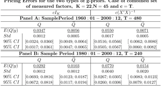
2. In order to compare the two favored models using the two different priors we first look at the pricing errors. Table 3 is a summary of the posterior means, standard deviation and confidence intervals for the pricing errors for the two types of priors. With the condition-ally independent prior, the mean pricing error for the most favored model with the factors

{V W RET , SP500, SM B, HM L}is 0.0056% forQe2_{(resp. 0.0347% forQ}2_{) compared to 0.0071%}

(resp. 0.055% forQ2_{) for the most favored model under the g-prior with factors{SM B, HM L}.}

The 4-factor APT shrinks the pricing error by about 21% (resp. 36% for Q2_{). To assess the}

economic importance of the pricing errors, we will follow Geweke & Zhou (1996) argument and compare the magnitude of the mean of Qwith the monthly expected returns. For the sample period 1960-2000, the means range from 0.7015 to 1.6584 percent per month. One can regard the above means of the pricing errors as economically negligible. To further assess the pricing error we provide the 90% (95%) Bayesian confidence interval, which state that that there is 90% (95%) probability that the pricing errors in the interval. The smaller the confidence interval,

the more heavily concentrated the posterior density of the average pricing error near its mean and the more informative are the data on the pricing error.

Pricing Errors for the two types of g-priors. Case of combined set of measured factors, K=22,N=45 and c=T.

cIK c(X0X)−1 Panel A: SamplePeriod 1960:01−2000:12, T=480 Q Qe Q Qe E(Q|y) 0.0347 0.0056 0.0550 0.0071 Std 0.0012 0.0005 0.0017 0.0005 90%CI [0.0324; 0.0360] [0.0049; 0.0064] [0.0516; 0.0566] [0.0062; 0.0080] 95%CI [0.0317; 0.0361] [0.0047; 0.0065] [0.0505; 0.0567] [0.0060; 0.0082]

Panel B: Sample Period 1980:01−2000:12, T=240

Q Qe Q Qe

E(Q|y) 0.0292 0.0103 0.0770 0.0154

Std 0.0012 0.0012 0.0040 0.0020

90%CI [0.0693; 0.0816] [0.0123; 0.0187] [0.0267; 0.0305] [0.0083; 0.0123]

95%CI [0.0672; 0.0818] [0.0117; 0.0194] [0.0260; 0.0306] [0.0079; 0.0127]

3. The average proportionD1 for the 4-factor model is 99.96% and an average of 93.34% for the proportion D2. The two-factor model has an average proportion of 99.74% for D1 and 49.02% forD2. Figure 1 andFigure 2 show that the 4-factor has both a higherD1 and D2 compared to the two-factor model for all asset returns in the sample. The higher the proportion D1, the smaller is the idiosyncratic risk relative to the systematic risk. Both models have proportions above 99.5%. However, the gap between the sample variances of the asset returns and the estimated total risk is far greater in the two-factor compared to the4-factor AP T.

4. In terms of matching the average returns,Figure 1 shows that the design matrix prior appears to produce estimates that are very similar to the classical approach. The independent prior. produces estimates for the expected returns that are quantitatively very low compared to the data dependent prior and the sample means.

Table 1: Estimates for Size Decile Portfolio Returns Factor Sensitivities and posterior probabilities for the period 1960 : 01-1989 : 12,cpm= 1.6989·103,T = 360,N = 10 andkmax= 14. The posterior meanE(δi|y) = 1, fori={M arket−Rf, SM B}. RT M SE = 0.0068

β0 βM arket−Rf βSM B decile1 0.0102 0.0320 0.0489 decile2 0.0083 0.0361 0.0443 decile3 0.0079 0.0382 0.0399 decile4 0.0081 0.0415 0.0359 decile5 0.0066 0.0421 0.0331 decile6 0.0066 0.0439 0.0276 decile7 0.0069 0.0450 0.0226 decile8 0.0054 0.0444 0.0185 decile9 0.0048 0.0459 0.0138 decile10 0.0030 0.0463 -0.0021 b δi 0.0083 -0.1006 0.0786 CI95% (0.0011 , 0.0173) (−0.2545 , 0.0471) (0.0123 , 0.1345)

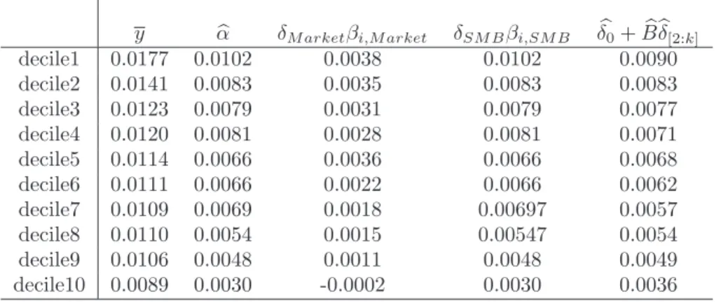
Table 2: Estimates for Expected Size Decile Portfolio Returns, and returns to factor risk exposure (δjβij) for the period 1960 : 01-1989 : 12,cpm= 1.6989·103, T = 360,N = 10 andkmax = 14. The posterior meanE(δi|y) = 1, fori={M arket−Rf, SM B}. RT M SE = 0.0068

y αb δM arketβi,M arket δSM Bβi,SM B δb0+Bbδb[2:k]

decile1 0.0177 0.0102 0.0038 0.0102 0.0090 decile2 0.0141 0.0083 0.0035 0.0083 0.0083 decile3 0.0123 0.0079 0.0031 0.0079 0.0077 decile4 0.0120 0.0081 0.0028 0.0081 0.0071 decile5 0.0114 0.0066 0.0036 0.0066 0.0068 decile6 0.0111 0.0066 0.0022 0.0066 0.0062 decile7 0.0109 0.0069 0.0018 0.00697 0.0057 decile8 0.0110 0.0054 0.0015 0.00547 0.0054 decile9 0.0106 0.0048 0.0011 0.0048 0.0049 decile10 0.0089 0.0030 -0.0002 0.0030 0.0036

Table 3: Ratios of Diagonal elements of the Sample covariance matrix of the Decile returnsdiag(Y0_Y N ) and the diagonal elements,diag(Bb0_X0_XBb

N ),anddiag(Σ) for the period 1960 : 01-1989 : 12,b cpm= 1.6989· 103_{,T = 360,N= 10,andk}

max= 14. The posterior meanE(δi|y) = 1, fori={M arket−Rf, SM B}.

RT M SE= 0.0068 Returns diag(Y0_Y N ) diag(Bb0X0XBb+Σ)b diag(Bb0X0XBb N ) diag(Y0Y N ) diag(Σ)b diag(Y0Y N ) decile1 0.2206 0.0320 0.7577 0.4558 decile2 0.1786 0.0107 0.9047 0.1277 decile3 0.1632 0.0209 0.9270 0.3706 decile4 0.1515 0.0069 0.9835 0.0659 decile5 0.1409 0.0208 1.0014 0.4332 decile6 0.1309 0.0132 0.9912 0.2657 decile7 0.1224 0.0254 0.9734 0.6560 decile8 0.1087 0.0046 0.9755 0.0576 decile9 0.0954 0.0188 1.0511 0.6097 decile10 0.0683 0.0287 1.0972 1.4073

Table 4: Estimates for Posterior probability ofγi for Economic Factors whenF ama0sthree Factors are ignored. The columns shows the estimates of the risk Premia and their Confidence interval. Sample period, 1960 : 01-1989 : 12,cpm= 2.5921,T = 360,N= 10 andkmax= 11

F actors γpm δbj 99%CI(δbj) Zero−β 1 0.0022 (0,0.0079) U T S 0.0735 -0.0062 (−0.2851,0.0292) P SAV E 0.2206 -0.0075 (−0.3409,0.2060) EI 0.0441 -0.0011 (−0.2163,0.0766) U EI 0.0588 0.0030 (−0.0852,0.1604)

Figure 1: Out of Sample forecasts for the Size Decile Portfolio Returns for the period 1990 : 01-1991 : 12, based on 1960 : 01-1989 : 12 In-sample data, cpm = 1.6989·103, T = 360, N = 10,and

kmax= 14. The posterior meanE(δi|y) = 1, fori={M arket−Rf, SM B}. RT M SE= 0.0068

1990:01 1990:06 1990:12 1991:06 1991:12 −0.2 0 0.2 1990:01 1990:06 1990:12 1991:06 1991:12 −0.2 0 0.2 1990:01 1990:06 1990:12 1991:06 1991:12 −0.2 0 0.2 1990:01 1990:06 1990:12 1991:06 1991:12 −0.2 0 0.2 1990:01 1990:06 1990:12 1991:6 1991:24 −0.2 0 0.2 1990:01 1990:06 1990:12 1991:06 1991:12 −0.2 0 0.2 1990:01 1990:06 1990:12 1991:06 1991:12 −0.2 0 0.2 1990:01 1990:06 1990:12 1991:06 1991:12 −0.2 0 0.2 1990:01 1990:06 1990:12 1991:06 1991:12 −0.2 0 0.2 1990:01 1990:06 1990:12 1991:06 1991:12 −0.2 0 0.2

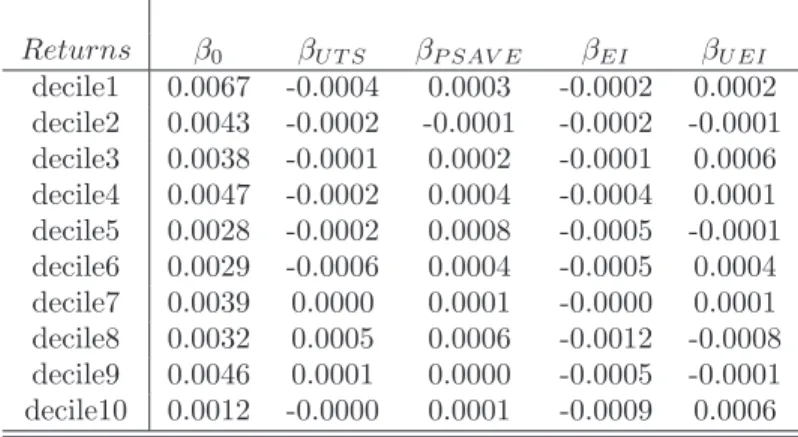
Table 5: Estimates for Size Decile Portfolio Returns Factor Sensitivities and posterior probabilities for the period 1960 : 01-1989 : 12,cpm= 2.5921,T = 360,N= 10 andkmax= 11.

Returns β0 βU T S βP SAV E βEI βU EI decile1 0.0067 -0.0004 0.0003 -0.0002 0.0002 decile2 0.0043 -0.0002 -0.0001 -0.0002 -0.0001 decile3 0.0038 -0.0001 0.0002 -0.0001 0.0006 decile4 0.0047 -0.0002 0.0004 -0.0004 0.0001 decile5 0.0028 -0.0002 0.0008 -0.0005 -0.0001 decile6 0.0029 -0.0006 0.0004 -0.0005 0.0004 decile7 0.0039 0.0000 0.0001 -0.0000 0.0001 decile8 0.0032 0.0005 0.0006 -0.0012 -0.0008 decile9 0.0046 0.0001 0.0000 -0.0005 -0.0001 decile10 0.0012 -0.0000 0.0001 -0.0009 0.0006

5

Conclusion

In this article, we propose a fully bayesian framework for selecting the risk factors and examining their risk premia and the pricing restrictions implied by the APT. This a one step approach which integrates the uncertainty behind model selection and the estimation of the different functions of the parameters. In contrast to existing studies, we do not fix a priori the number of measured variables allowed to enter the pricing relationship. The number of measured variables and statistical factors is endogenously determined . This process is performed simultaneously with the estimation of the factor betas and their risk premia. Hence, this method avoids the errors in variables problem encountered in the main stream two-pass approach of Fama-MacBeth. Because, the bayesian approach evaluates the exact posterior distribution of the estimated parameters and any other function of the parameters, we

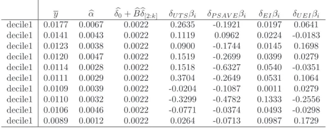
Table 6: Estimates for Expected Size Decile Portfolio Returns, and returns to factor risk exposure (δjβij) for the period 1960 : 01-1989 : 12,cpm= 2.5921,T = 360,N = 10 and kmax = 11. Note: The returns to individual factor riskδjβi should be (×10−5).

y αb δb0+Bbbδ[2:k] δU T Sβi δP SAV Eβi δEIβi δU EIβi decile1 0.0177 0.0067 0.0022 0.2635 -0.1921 0.0197 0.0641 decile1 0.0141 0.0043 0.0022 0.1119 0.0962 0.0224 -0.0183 decile1 0.0123 0.0038 0.0022 0.0900 -0.1744 0.0145 0.1698 decile1 0.0120 0.0047 0.0022 0.1519 -0.2699 0.0399 0.0279 decile1 0.0114 0.0028 0.0022 0.1518 -0.6327 0.0540 -0.0351 decile1 0.0111 0.0029 0.0022 0.3704 -0.2649 0.0531 0.1064 decile1 0.0109 0.0039 0.0022 -0.0204 -0.1087 0.0011 0.0279 decile1 0.0110 0.0032 0.0022 -0.3299 -0.4782 0.1333 -0.2556 decile1 0.0106 0.0046 0.0022 -0.0771 -0.0374 0.0493 -0.0298 decile1 0.0089 0.0012 0.0022 0.0264 -0.0713 0.0987 0.1729

Table 7: Ratios of Diagonal elements of the Sample covariance matrix of the Decile returnsdiag(Y0_Y N ) and the diagonal elements,diag(Bb0_X0_XBb

N ),anddiag(Σ) for the period 1960 : 01-1989 : 12,b cpm= 2.5921,

T = 360,N = 10,andkmax= 11. Returns diag(Y0_Y N ) diag(Bb0X0XBb+Σ)b diag(Bb0X0XBb N ) diag(Y0Y N ) diag(Σ)b diag(Y0Y N ) decile1 0.2206 0.0030 0.0001 0.4963 decile2 0.1786 0.0027 0.0000 0.5507 decile3 0.1632 0.0021 0.0001 0.4705 decile4 0.1515 0.0028 0.0001 0.6808 decile5 0.1409 0.0029 0.0002 0.7417 decile6 0.1309 0.0019 0.0004 0.5305 decile7 0.1224 0.0010 0.0000 0.2969 decile8 0.1087 0.0021 0.0002 0.6865 decile9 0.0954 0.0028 0.0000 1.0846 decile10 0.0683 0.0023 0.0011 1.2405

Table 8: Estimates for Posterior probability of γi for Factors Pervasive for the Industry Portfolios Returns. The columns shows the estimates of the risk Premia and their Confidence interval. Sample period, 1960 : 01-1989 : 12,cpm= 0.0072,T = 360,N = 12 andkmax= 11

F actors γpm δbj 95%CI(δbj) Zero−β 1 0.0045 (0.0043,0.0046) JAN 0.5556 -0.1347 (−0.8087,0.0000) CG 0.8333 0.0352 (0.0000,0.1249) U T S 0.5 -0.0100 (−0.0604,0.0000) U RP 0.3333 -0.0201 (−0.1209,0.0000) U N EM−1 0.3333 0 N A EI 0.5 0.2195 (0.0000,1.317) M ark−Rf 0.6666 0.0218 (0.0000,0.1309) SM B 0.5 -0.1239 (−0.7437,0.0000) HM L 0.5 -0.0007 (−0.0043,0.0000)

Table 9: Estimates for Industry Portfolio Returns Factor Sensitivities for the period 1960 : 01-1989 : 12,cpm= 2.5921,T = 360,N = 12 andkmax= 11.

Returns βJAN βCG βU T S βU RP βEI βM ark−Rf βSM B βHM L

N onDur -0.0001 -0.0000 0.0000 0.0001 0.0003 -0.0002 -0.0000 0.0001 Durabl 0.0000 -0.0001 0.0003 0.0002 -0.0000 0.0000 -0.0001 0.0001 M anuf c -0.0001 -0.0002 -0.0001 0.0002 -0.0001 -0.0001 -0.0001 -0.0000 Energy -0.0000 0.0001 -0.0003 0.0001 0.0001 -0.0002 0.0001 -0.0002 Chemis -0.0000 -0.0000 -0.0001 0.0000 0.0001 -0.0002 -0.0001 -0.0000 BusEqu -0.0001 0.0008 -0.0001 0.0000 -0.0002 -0.0003 0.0001 -0.0002 T eLcm -0.0001 -0.0001 0.0002 0.0002 0.0001 -0.0001 0.0001 -0.0000 UtiLis -0.0000 0.0002 0.0001 0.0001 0.0000 0.0001 0.0001 0.0001 Shops 0.0001 0.0001 0.0001 0.0002 -0.0001 0.0003 0.0001 -0.0000 Health 0.0000 -0.0013 0.0002 -0.0003 0.0001 0.0003 -0.0001 0.0000 M oney -0.0001 0.0001 0.0000 0.0003 0.0001 0.0001 -0.0000 0.0000 Other 0.0000 -0.0003 0.0000 -0.0001 0.0000 -0.0001 0.0000 -0.0001

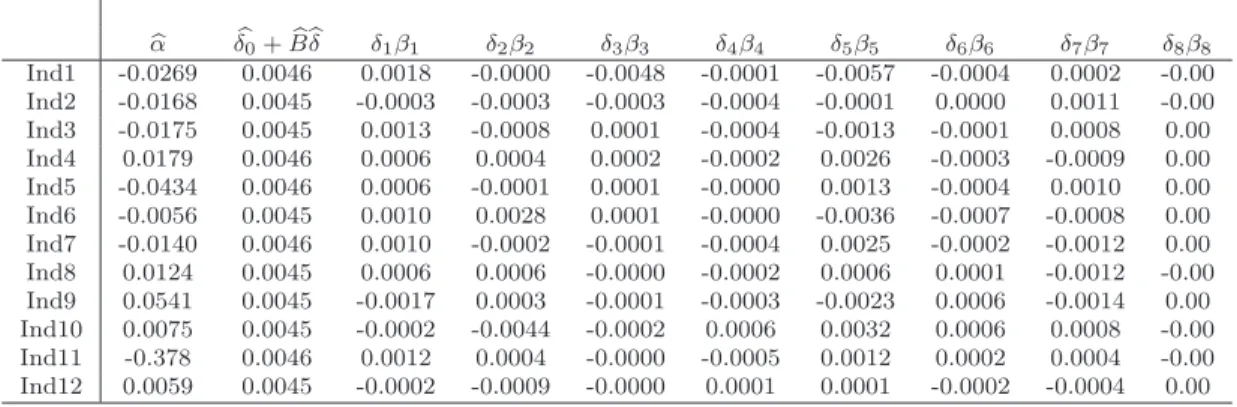
Table 10: Expected Industry Portfolio Returns, and returns to factor risk exposure (in % )(δjβij) for the period 1960 : 01-1989 : 12,cpm= 0.0072, T= 360,N = 12 andkmax= 11.

b α δb0+Bbbδ δ1β1 δ2β2 δ3β3 δ4β4 δ5β5 δ6β6 δ7β7 δ8β8 Ind1 -0.0269 0.0046 0.0018 -0.0000 -0.0048 -0.0001 -0.0057 -0.0004 0.0002 -0.00 Ind2 -0.0168 0.0045 -0.0003 -0.0003 -0.0003 -0.0004 -0.0001 0.0000 0.0011 -0.00 Ind3 -0.0175 0.0045 0.0013 -0.0008 0.0001 -0.0004 -0.0013 -0.0001 0.0008 0.00 Ind4 0.0179 0.0046 0.0006 0.0004 0.0002 -0.0002 0.0026 -0.0003 -0.0009 0.00 Ind5 -0.0434 0.0046 0.0006 -0.0001 0.0001 -0.0000 0.0013 -0.0004 0.0010 0.00 Ind6 -0.0056 0.0045 0.0010 0.0028 0.0001 -0.0000 -0.0036 -0.0007 -0.0008 0.00 Ind7 -0.0140 0.0046 0.0010 -0.0002 -0.0001 -0.0004 0.0025 -0.0002 -0.0012 0.00 Ind8 0.0124 0.0045 0.0006 0.0006 -0.0000 -0.0002 0.0006 0.0001 -0.0012 -0.00 Ind9 0.0541 0.0045 -0.0017 0.0003 -0.0001 -0.0003 -0.0023 0.0006 -0.0014 0.00 Ind10 0.0075 0.0045 -0.0002 -0.0044 -0.0002 0.0006 0.0032 0.0006 0.0008 -0.00 Ind11 -0.378 0.0046 0.0012 0.0004 -0.0000 -0.0005 0.0012 0.0002 0.0004 -0.00 Ind12 0.0059 0.0045 -0.0002 -0.0009 -0.0000 0.0001 0.0001 -0.0002 -0.0004 0.00

Table 11: Ratios of Diagonal elements of the Sample covariance matrix of the Industry returns diag(Y0_Y

N ) and the diagonal elements, diag(

b

B0_X0_XBb

N ),and diag(Σ) for the period 1960 : 01-1989 : 12,b

cpm= 0.0072,T = 360,N = 12,andkmax= 11. Returns diag(Y0_Y N ) diag(Bb0X0XBb+Σ)b diag(Bb0X0XBb N ) diag(Y0Y N ) diag(bΣ) diag(Y0Y N ) N onDur 0.0022 0.0029 0.0001 1.3177 Durabl 0.0030 0.0004 0.0001 0.1254 M anuf c 0.0027 0.0002 0.0000 0.0816 Energy 0.0028 0.0022 0.0000 0.7752 Chemis 0.0024 0.0010 0.0000 0.4336 BusEqu 0.0034 0.0015 0.0002 0.4522 U tiLis 0.0016 0.0023 0.0001 1.4392 Shops 0.0031 0.0007 0.0001 0.2152 Health 0.0029 0.0016 0.0006 0.5539 M oney 0.0026 0.0003 0.0001 0.1210 Other 0.0032 0.0012 0.0000 0.3818

are able to produce bayesian confidence intervals for the risk premia to gage if the market does price a certain factor. Inference is also done on the average pricing errors in order to evaluate the extent to which the APT restrictions deviate from the data. In an APT with only measured economic variables are allowed along with Fama and French three factors, the choice of the prior on the factor betas influences the posterior distribution of the promising factors. In the case of Zellner g-prior where the

Table 12: Estimates for the Pricing Error (in %) for the period 1960 : 01-1989 : 12, cpm = 0.0072,

T = 360,N = 12,andkmax= 11.

E(.) std(.) CI(95%) Q2 _{0.0014 0.0028 (0 , 0.0076)}

Q 0.0191 0.0321 (0 , 0.0874)

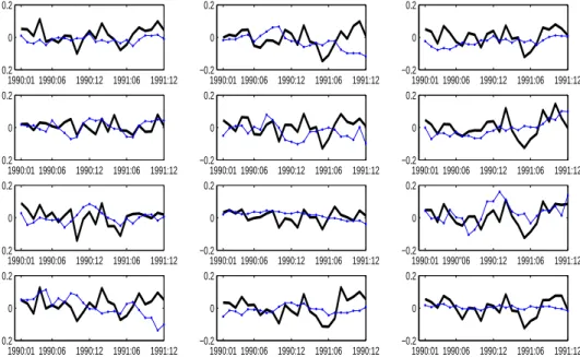
Figure 2: Out of Sample forecasts for the Industry Portfolio Returns for the period 1990 : 01-1991 : 12, based on 1960 : 01-1989 : 12 In-sample data, cpm = 0.0072, T = 360, N = 12,and kmax = 14.

RT M SE= 0.0503 1990:01 1990:06 1990:12 1991:06 1991:12 −0.2 0 0.2 1990:01 1990:06 1990:12 1991:06 1991:12 −0.2 0 0.2 1990:01 1990:06 1990:12 1991:06 1991:12 −0.2 0 0.2 1990:01 1990:06 1990:12 1991:06 1991:12 −0.2 0 0.2 1990:01 1990:06 1990:12 1991:06 1991:12 −0.2 0 0.2 1990:01 1990:06 1990:12 1991:06 1991:12 −0.2 0 0.2 1990:01 1990:06 1990:12 1991:06 1991:12 −0.2 0 0.2 1990:01 1990:06 1990:12 1991:06 1991:12 −0.2 0 0.2 1990:01 1990"06 1990:12 1991:06 1991:12 −0.2 0 0.2 1990:01 1990:06 1990:12 1991:06 1991:12 −0.2 0 0.2 1990:01 1990:06 1990:12 1991:06 1990:12 −0.2 0 0.2 1990:01 1990:06 1990:12 1991:06 1991:12 −0.2 0 0.2

prior covariance matrix is a replica of the design matrix, the pervasive factors are Fama and French size and book to market risk factors SM B and HM L. However, using the conditionally dependent prior, in addition to SM B and HM L,some economic variables appear to be priced by the market. More specifically, inflation, unexpected inflation, return on value-weighted portfolio and return on the standard and poor portfolio.

References

[1] Anderson, T. W. and Amemiya, Y., (1988), The Asymptotic Normal Distribution of Estimators in Factor Analysis under General Conditions,Annals of Statistics, Vol. 16, 759-771

[2] Bartlett, M. (1957), A comment on D. V. Lindley’s Statistical Paradox.Biometrika Vol. 44, pp. 533-534

[3] Berger, J. O., Ghosh, J. K. and Mukhopadhyay, N. (2003), Approximations and Consistency of Bayes Factors as Model Dimension Grows. Journal of Statistical Planning and Inference, Vol. 112, pp. 241-258.

[4] Brown, P. J., Vannucci, M. and Fearn, T. (1998), Multivariate Bayesian Variable Selection and Prediction,Journal of the Royal Statistical Society, series B, Vol. 60, Part 3, pp. 627-641

[5] Brown, P. J., Vannucci, M. and Fearn, T. (1999), The Choice of Variables in Multivariate Regres-sion: A Non-conjugate Bayesian Decision Theory Approach.Biometrika Vol. 86, pp. 635-648

[6] Burmeister, E. and McElroy, B. M.,(1988), Joint Estimation of Factor Sensitivities and Risk Premia for the Arbitrage Pricing Theory.Journal of Finance, Vol. XLIII, No. 3, pp. 721-733.

[7] Carlin, B. P. and Chib, S. (1995), Bayesian Model Choice Via Markov Chain Monte Carlo Meth-ods.Journal of the Royal Statistical Society, Series B, Vol. 57, pp. 473-484.

[8] Chamberlin, G. and Rothschild, M. (1983), Arbitrage, Factor Structure and Mean-Variance Anal-ysis in Large Asset Markets, Econometrica 51,1305-1324.

[9] Chen, N. F., Roll, R. and Ross, S., A. (1986), Economic Forces and the Stock Market,Journal of Business Vol. 59, pp. 383-403.

[10] Chipman H., George E. I. and McCulloch R. E. (2001), The Practical Implementation of Bayesian Model Selection,ims Lecture Notes- Monograph Series, Vol. 38, pp. 65-134.

[11] Donoho, D. L. and Johnstone, I.M. (1994), Ideal Spatial Adaptation by Wavelet Shrinkage,

Biometrika, Vol. 81, pp. 425-456/

[12] Fama, E. F., and French, K. R. (1993), Common Risk Factors in the Returns on Stocks and Bonds,Journal of Financial Economics Vol. 33, No. 1, pp. 3-56.

[13] Ferson, E. W., and Harvey, R. C. (1991), The Variation of Economic Risk Premiums,Journal of Political Economy, Vol. 99, No. 2, pp. 385-415.

[14] Foster, D. P., and George, E. I. (1994),The Risk Inflation Criterion for Multiple Regression,The Annals of Statistics, Vol. 22, pp. 1947-1975

[15] George, E. and McCulloch, R. E. (1993), Variable Selection Via Gibbs Sampling.Journal of the American Statistical Association, Vol. 88, pp. 881-889

[16] Geweke, J. and Zhou, G., (1996), Measuring the Pricing Error of the Arbitrage Pricing Theory,

The Review of Financial Studies, Vol.9, N0. 2, 557-587

[17] Ouysse, R., (2006), Consistent Variable Selection In Large Panels When Factors are Observable,

Journal of Multivariate Analysis, Vol. 97, pp. 946-984.

[18] Liang F., Paulo R., Molina G., Clyde M. A. and Berger J., (2007), Mixtures of g-priors for Bayesian Variable Selection,Unpublished Manuscript.

[19] Smith, M. and Kohn, R. (1996), Nonparametric Regression using Bayesian Variable Selection.

Journal of Econometrics, Vol. 75, pp. 317-343.

[20] Smith, M. and Kohn, R. (1997), A Bayesian Approach to Nonparametric Bivariate Regression.

Journal of the American Statistical Association, Vol. 92, pp. 1522-1535.

[21] Smith, M. and Kohn, R. (2002), Parsimonious Covariance Matrix Estimation for Longitudinal Data.Journal of the American Statistical Association, Vol. 97, pp. 1141-1153.

6

APPENDIX:

6.1

Data Appendix

6.1.1 Fama and French Portfolio Factors.

First the stock returns are ranked on size (prices times shares). The median size is then used to split the stocks into two groups, small and big (S and B). The returns are also broken into three book-to-market groups based on the bottom 30% (L), middle 40% (M) and the top 30% (H). Six portfolios (S/L, S/M, S/H, B/L, B/M, B/H) are then constructed from the intersection of the two size groups and the threeBE/M E groups. Two additional portfolios are constructed from these intersections. HM L (high minus low) meant to mimic the risk factor in return related to book to market equity BE/M E. It is defined as the difference between the average return on the two

high-BE/M E portfolios and the average returns on the two low-BE/M E. The portfolio SM B (small minus big) meant to mimic the risk factor in return related to size. It is the difference between small and big stocks with about the same book to market equity. Finally, a value-weighted portfolio on the six size-BE/M E portfolio to proxy for market factor. To simplify notations, the set of factors used in Fama and French (1993) will be denotedFF F_.

6.1.2 Chen, Roll and Ross macroeconomic factors

From Roll and Ross (1986), the following set of variables is constructed:

- Consumption growth CG: growth rate in real per capita consumption constructed by dividing the series of seasonally adjusted real personal consumption (excluding durables) by the population. The series are fromF RED (Federal reserve bank of St. Louis).

- Term structure of interest rate U T S: the spread between the return on a long term government bond and the lagged return on one month bills. The two series are from CRSP US Treasury and Inflation Indices.

- Risk premiumU RP: the spread between the return on low grade bonds (Moody’s seasonally adjusted

Baacorporate bond yield) and a long term government bond.

- Monthly growth of industrial production M P(t): measured the change in industrial production lagged by one month.

- Annual growth of industrial productionY P(t).

- Oil price growth OG: the producer price index for crude petroleum. Source: Bureau of Labor Statistics.

- Expected inflationEI(t): constructed using Fama and Gibbons (1984).

- Unexpected inflationU EI(t) =I(t)−E(I(t)|t−1).

- Change in expected inflationDEI(t) =E(I(t+ 1)|t)−E(I(t|t−1)).

- Financial market indices: the return on value weightedV W RET Dand equally weightedEW RT D

portfolios ofN Y SElisted stocks.

To these variables, an additional set of potential sources of variation are added:

- The unemployment rateU N EM P :Civilian unemployment rate percent, seasonally adjusted. Source: Bureau of Labor Statistics (F RED).

- The growth rate of money base GB :Currency component of money stock plus demand deposits seasonally adjusted (F RED).

- Private saving rate P SAV E :Percent, seasonally adjusted. All the variables used in CRR are collected in a set denoted byFRR_.

• where λ=vec(Λ); thus Λ

(N×r)= (λ1, .., λ(r×1)i .., λN) 0_.

6.2

Proofs

6.2.1 Gibbs Sampler

The Gibbs sampler generates an ergodic Markov chain,

γ(0)_{, γ}(1)_,Ω(1)_{, β}(1)_{, ....γ}(j)_,Ω(j)_{, β}(j)_,...,γ(M)_,Ω(M)_{, β}(M)

Except forγ(0) _{which is initialized asγ}(0)_{= (1,0,0, ...,0), the subsequent values ofγ}(j)_,Ω(j)_{, β}(j)_are

obtained obtained by successively simulationg values according to the following iterated scheme.

1. Given γ(j−1)_{,the next iterateγ}(1) _{is obtained by sampling fromp(γ|y, X)}

pk = P(γk= 1|γ/k, y, X) = L 1 +L L ∝ à ¯ ¯_Hβ(1)¯¯ ¯ ¯_Hβ(0)¯¯ !−N 2   ¯ ¯ ¯X0 γ(1)Xγ(1)+Hβ(1)−1 ¯ ¯ ¯ ¯ ¯ ¯X0 γ(0)Xγ(0)+Hβ(0)−1 ¯ ¯ ¯   −N 2 _µ |Φ +S(1)| |Φ +S(0)| ¶−(T+m) 2 Drawu∼U(0,1) if u < pk thenγk(j)= 1;γ(j)=γ(1) andS (j)_=S(1) (a) else γ_k(j)= 0;γ(j)_=γ (0)andS (j)_{=S(0)end else}

2. Given γ(j)_{, draw Ω}(j) _{by sampling from the Wishart distribution Ω}(j)_{|y, γ}(j) _{∼ W}

N(m+

T,¡S(γ(j)_{) + Φ}¢−1_{), where}

S(γ(j)_{) = Y}0³_I

T −Xγ(j)D_γ−1(j)X_γ0(j)

´

Y if we take a prior withβ0=0

Dγ(j) =

³

X0

γ(j)Xγ(j)+H−1_β

´

3. Given γ(j)_{, Ω}(j)_{, draw β}(j) _{by random sampling from β}(j)_|y,Ω(j)_{, γ}(j) _{∼ N}³_βe

γ,Σ(j)⊗D−1_γ(j) ´ where Σ(j)₌¡_Ω(j)¢−1 _and e β_γ(j)= ³ IN⊗D−1_γ(j)H−1β ´ β0+ ³ IN ⊗D−1_γ(j)X_γ0(j)X_γ(j) ´ b βGLS

4. Compute the risk premia iterates δ(j)₌³_Be(j)0_e

B(j)´−1_Be(j)0_α(j) _{and the pricing errors iterates}

e Q2(j) N = α(j)0 µ IN −Be(j) ³ e B(j)0_e B(j)´−1_Be(j)0 ¶0 Ω(j) µ IN −Be(j) ³ e B(j)0_e B(j)´−1_Be(j)0 ¶ α(j) N e B(j) _{= (ı,Be}(j)₎ Q2(j) N = α(j)0 µ IN −Be(j) ³ e B(j)0_e B(j)´−1_Be(j)0 ¶ α(j) N

6.2.2 Posterir density of γ|y, X

For the Normal-Wishart g-prior case, the random mechanism general informative prior (See Ap-pendix), L = p[γ(1)|y] p[γ(0)|y] ∝ p(y|γ(1)) p(y|γ(0)) ∝ à ¯ ¯_Hβ(1)¯¯ ¯ ¯_Hβ(0)¯¯ !−N 2   ¯ ¯ ¯X0 γ(1)Xγ(1)+Hβ(1)−1 ¯ ¯ ¯ ¯ ¯ ¯X0 γ(0)Xγ(0)+Hβ(0)−1 ¯ ¯ ¯   −N 2 _µ |Φ +S(1)| |Φ +S(0)| ¶−(T+m) 2 logL = −N 2 log ¯ ¯_Hβ(1)¯¯ ¯ ¯_Hβ(0)¯¯− N 2 log ¯ ¯ ¯X0 γ(1)Xγ(1)+Hβ(1)−1 ¯ ¯ ¯ ¯ ¯ ¯X0 γ(0)Xγ(0)+Hβ(0)−1 ¯ ¯ ¯ −(T+m) 2 log |Φ +S(1)| |Φ +S(0)| (16)

In the informative diffuse prior case 1:

L∝c−N2   ¯ ¯ ¯X0 γ(1)Xγ(1)+1cIqγ(1) ¯ ¯ ¯ ¯ ¯ ¯X0 γ(0)Xγ(0)+1cIqγ(0) ¯ ¯ ¯   −N 2 _µ |Φ +S(1)| |Φ +S(0)| ¶−(T+m) 2 logL=−N 2 logc− N 2 log ¯ ¯ ¯X0 γ(1)Xγ(1)+1cIqγ(1) ¯ ¯ ¯ ¯ ¯ ¯X0 γ(0)Xγ(0)+1cIqγ(0) ¯ ¯ ¯− (T+m) 2 log ¯ ¯_{Sγ(1)+ Φ}¯¯ ¯ ¯_{Sγ(0)+ Φ}¯¯ (17)