Explaining policy volatility
in developing countries
Vatcharin Sirimaneetham
Discussion Paper No. 06/583
February 2006
Department of Economics
University of Bristol
8 Woodland Road
Bristol BS8 1TN
Explaining policy volatility
in developing countries
∗
Vatcharin Sirimaneetham
†Department of Economics, University of Bristol
8 Woodland Road, Bristol BS8 1TN, UK
February 28, 2006
Abstract
This paper studies the causes of policy volatility in developing coun-tries during 1970-1999. To construct composite policy volatility indi-cators, the paper applies a robust principal components analysis to Washington Consensus policy variables. The results suggest three di-mensions of policy volatility: Þscal, macroeconomic and development policies. The paper shows that more stable macroeconomic policy is associated with higher income growth, before turning to the determi-nants of volatility. Using a Bayesian approach which addresses the model uncertainty problem, the paperÞnds that macroeconomic pol-icy is more volatile in countries that adopt a presidential system, have weaker political constraints, where government stability is lower, and that are former British colonies. Adopting a parliamentary regime helps to stabilize policy.
JEL ClassiÞcations: C11, O11, O40
Keywords: policy volatility, economic growth, Bayesian model averaging, principal components
∗I am grateful to Jonathan Temple for various useful comments and suggestions, and to Daron Acemoglu, Kenneth Bollen, Daniel Treisman and Halit Yanikkaya for making their data available. The usual disclaimer applies.
1
Introduction
It is widely believed that the volatility of macroeconomic variables such as
Þscal deÞcits and the real exchange rate is bad for income growth. But why some countries experience more volatile government policies than others is less well understood. Partly this is because much of the past literature has focused on a limited set of possible explanations. The literature on the determinants of inßation and real exchange rate volatility, for example, is mainly dominated by the role of trade openness.
Recent papers such as Acemoglu et al. (2003) and Easterly (2005) argue that sound macroeconomic policy appears to contribute to economic growth only because it is a proxy for good institutions.1 Fatás and Mihov (2005) show that if we measure macroeconomic policy in term of its volatility rather than its level, macroeconomic policy volatility directly matters for growth. This emphasizes the importance of seeking to explain policy volatility.
An ability to explain policy volatility is especially important for devel-oping countries. Table 1 shows that low-income countries experienced more volatile macroeconomic and development policies in the past three decades. Although theirÞscal policy was not excessively volatile compared to devel-oped countries, the ability to maintain price and real exchange rate stability was much poorer. Table 1 also documents that low-income countries expe-rienced more volatile growth rates.
This paper seeks to explain why some developing countries had more volatile government policies than others during 1970-1999. IÞrst construct new composite indicators of policy volatility by applying the method of prin-cipal components to a set of Washington Consensus policy variables. The results suggest three dimensions of policy volatility indicators, namely, Þ s-cal deÞcit volatility, macroeconomic policy volatility and development pol-icy volatility. These indicators are available for 87, 72 and 65 developing countries, respectively. Note that macroeconomic policy volatility reßects
1
In particular, when institutional variables are also included in growth regressions, the explanatory power of policy variables is less strong. Using Bayesian methods, Sirima-neetham and Temple (2006) provide some evidence that sound macroeconomic policy is associated with higher income growth in developing countries even after controlling for a range of institutional variables and other growth determinants.
an unstable inßation rate and real exchange rate, while development policy volatility reßects changes in liberalization policies in the areas of interna-tional trade, government regulation and the protection of property rights.
Using standard growth regressions, I then show that income per capita growth is negatively associated with macroeconomic policy volatility during 1970-1999. The strength of the association is also sizeable. A one-standard-deviation decrease in macroeconomic policy volatility raises growth by 0.63-0.73 percentage points. This negative relationship remains strong even when proxies for the quality of institutions are also included. I howeverÞnd that unstableÞscal deÞcits and variation in development policy do not have much explanatory power for growth.
One can imagine that there are many variables which could potentially explain policy volatility, while there seems to be no established theories that guide how these variables may affect policy volatility. This implies that the model uncertainty problem is likely to prevail in this context. This paper adopts a Bayesian model averaging (BMA) approach to deal with the model uncertainty problem.
The Bayesian method allows us to consider a much wider range of pos-sible explanatory variables compared to the existing research. My preferred model considers 44 possible variables. Since the main focus is on a political economy approach, many of these variables are political variables, although I also investigate the roles of social and pre-determined factors such as media development and social heterogeneity.
The key Þndings of the paper are that macroeconomic policy is more volatile in countries that adopt a presidential system, have weaker execu-tive constraints in the policy-making process, where government stability is lower, and where electoral outcomes are less competitive. Countries which are former British colonies and have a larger population also experience less stable policy. Finally, adopting a parliamentary regime helps to stabilize policy. The size of these associations is notable. A one-standard-deviation change in these variables results in a 0.40-0.57 standard deviation change in macroeconomic policy volatility.
The rest of the paper is organized as follows. Section 2 brießy reviews the literature on the growth effects and determinants of policy volatility.
Sec-tion 3 describes the proxies for Washington Consensus policy indicators and some key explanatory variables. Section 4 discusses the concept of Bayesian model averaging (BMA). Section 5 brießy explains principal components analysis and describes the construction of composite policy volatility indica-tors. Section 6 reports the relationship between policy volatility indicators and income per capita growth. Section 7 presents the Þndings from BMA and then tests whether the independent variables suggested by BMA can explain policy volatility in a more orthodox regression analysis. The Þnal section concludes.
2
Causes and E
ff
ects of Policy Volatility
This section reviews the literature on growth and investment effects of policy volatility and socio-political determinants of policy volatility. It does not however cover the related literature on output volatility.2
2.1
Macroeconomic Policy Volatility
Much of the empirical work on the effects of macroeconomic policy volatility tests the investment theory proposed by Dixit and Pindyck (1994) where, in an uncertain policy environment, investors might delay investment as a result of irreversibility and uncertainty of Þxed projects. This could result in slower growth rates.3
The link between macroeconomic policy volatility and investment and growth is widely studied. One robustÞnding is that volatile real exchange rates are associated with lower output growth and a lower share of invest-ment in output.4 For example, Brunetti (1998) shows that only the negative relationship between Dollar (1992)’s real exchange rate distortion index and growth is robust in an extreme bound analysis, which also includes other
2See Ramey and Ramey (1995), Easterly et al. (2000), Imbs (2004), Hnatkovska and
Loayza (2004), Malik and Temple (2005), Raddatz (2005), Breen and García-Peñalosa (2005), Anbarci et al. (2005), Koren and Tenreyro (2005), and Spiliopoulas (2005).
3
More recent theoretical work includes Hopenhayn and Muniagurria (1996), Jeong (2002) and Varvarigos (2005).
4
See Servén and Solimano (1993), Servén (1998), Brunetti and Weder (1998), Bleaney (1996), and Bleaney and Greenaway (2001).
policy measures such asÞscal deÞcits, the inßation rate, and the black mar-ket premium. Various papers argue that macroeconomic policy uncertainty should affect only private investment, not government investment. Aizen-man and Marion (1999) provide supportive evidence by showing that volatil-ity in the real exchange rate, government consumption, and money growth lowers the private investment rate, but not total investment.
Another common Þnding in the literature is that inßation and money growth volatility do not seem to affect growth and investment.5 Moreover, unlike stability in real exchange rates, stability in the inßation rate does not appear to help to reduce poverty (Agénor, 2004).
In general, the literature suggests that Þscal policy volatility in term of unstable government consumption has a negative effect on growth in devel-oping countries (Aizenman and Marion (1993) and Turnovsky and Chat-topadhyay (2003)). This link however disappears when using government budget deÞcit volatility as a proxy. Fatás and Mihov (2005) constructed a measure of discretionary Þscal policy volatility, deÞned as the share of government consumption in output that is not predicted by government consumption in earlier periods and other control variables such as income and the inßation rate. They Þnd that this measure has a direct, negative effect on growth.
While most studies are concerned with more than one type of policy volatility, an attempt to combine them is not common. An exception is El-badawi and Schmidt-Hebbel (1998), which constructs an indicator of
macro-Þnancial volatility. This measure is a simple average of the standard devi-ations of public sector deÞcits, reserve money stock growth, real exchange rate, and current account deÞcits. They however Þnd that this composite measure lacks explanatory power for growth.
Fewer studies attempt to explain cross-country variation in macroeco-nomic policy volatility. The role of trade openness dominates the research that tries to explain real exchange rate volatility. Hau (2002) argues that a more open economy should experience less volatile real exchange rates
be-5
See Servén (1998), Brunetti (1998), Brunetti and Weder (1998), and Aizenman and Marion (1993). Exceptions include Servén and Solimano (1993) and Turnovsky and Chat-topadhyay (2003).
cause imported goods should help an economy to adjust its domestic price level more quickly during shock periods. This therefore reduces the real effects of shocks on consumption and the real exchange rate. Using export and import values as a proxy for trade openness, he Þnds supporting ev-idence for this argument. Calderón (2004) reports the same results when measuring trade openness by the Sachs and Warner (1995) index of trade policy.
Placing more emphasis on pre-determined factors, Bravo-Oetega and di Giovanni (2005) show that higher trade costs, as measured by distance be-tween a particular country and its trading partners, raise real exchange rate volatility because higher costs result in a larger non-tradable sector. Finally, Satyanath and Subramanian (2004) show that nominal parallel market ex-change rates are more volatile in countries that have lower international trade relative to GDP, a more unequal income distribution, and weaker con-straints on the executive.
The degree of trade openness is also used to explain inßation volatility. Bowdler and Malik (2005) show that trade openness helps to stabilize the inßation rate because it reduces volatility in money growth. Lo, Wong and Granato (2003) obtained similar results. Both studiesÞnd that this negative link is stronger in developing countries.
Much of the literature that explains Þscal policy volatility follows two lines of enquiry. TheÞrst group emphasizes the role of political constraints and Þnds that stronger constraints on executives tend to limit their power in implementing discretionaryÞscal policy (Fatás and Mihov (2003, 2004)). They also Þnd that countries that adopt a presidential regime in general experience more volatile government spending while electoral rules and the frequency of elections have limited explanatory power. Henisz (2004) reports similar results when using government subsidies and transfers, and capital expenditures as proxies forÞscal policy volatility.
The second body of research focuses on the detrimental role of social fragmentation on political instability, which leads to volatile Þscal policy. Dutt and Mitra (2004) Þnd that government consumption is more stable in countries with lower political instability, deÞned as a lower probability of regime switch between democracy and dictatorship. Woo (2003) also reveals
that public sector deÞcits are more volatile with a less equal income distri-bution. He however discovers no association betweenÞscal policy volatility and a political instability index.6
On a wider perspective, Ali and Isse (2004) document that more demo-cratic countries seem to enjoy more stable macroeconomic policy in terms of public sector debts, Þscal deÞcits, deposit interest rates, inßation rates, and a real effective exchange rate index.
2.2
Development Policy Volatility
Research on the volatility of development policy mainly focuses on growth and investment effects of the uncertainty of government regulations and protection of property rights. Pitlik (2002) shows that volatile liberalization policies, as measured by the uncertainty of the economic freedom index from the Fraser Institute, reduce growth even though the long run path is towards a more liberalized economy.7 A stable liberalization policy is also shown to be more important to growth than an improvement in policy over time. Dawson (2005) alsoÞnds that a volatile government regulations score from the Fraser Institute index is associated with slower growth.
Using aÞrm-level survey in 73 countries, Brunetti, Kisunko and Weder (1998) test whether uncertainty in government rules affects growth and in-vestment. They show that more stable judicial enforcement promotes growth and investment. The result is less strong for the uncertainty associated with rule making by the government.
Finally, unstable trade policy, as measured by the volatility of taxes on international trade, does not seem to affect growth (Brunetti, 1998). Trade policy becomes more stable with lower political instabilty (Dutt and Mitra, 2004) and stronger constraints on the executive (Henisz, 2004).
6The index is derived from a principal components method and includes the frequencies
of political assassinations, government crises, cabinet changes, and military coups.
7The Fraser Institute’s composite index covers various aspects of an economy including
government consumption, price stability, freedom of international trade, freedom of capital andÞnancial markets, and the protection of property rights. It is therefore a measure of both macroeconomic and development policies.
3
The Data
This section Þrst discusses proxies for Washington Consensus policy vari-ables. These variables will be used to construct new composite policy volatil-ity indicators in section 5.2. It then highlights some key independent vari-ables that could potentially explain policy volatility.
3.1
The Dependent Variables
To construct new composite indicators of policy volatility, I follow the idea of the Washington Consensus as summarized by Williamson (1990) and Fischer (2003). The Consensus consists of ten policy areas includingÞscal discipline, interest rate liberalization, a competitive exchange rate, tax reform, public expenditure prioritization, liberalized trade policy, foreign direct investment promotion, privatization, deregulation, and protection of private property rights. I add a low inßation rate into this list. The sample covers developing countries where the population size in 1970 was greater than 250,000 but excluding transition economies. The sample period is 1970-1999.
Unless otherwise stated, I always measure the degree of policy volatility by the natural logarithm of the standard deviation of policy variables over 1970-1999. Another commonly used method is to use the standard devia-tions of the residuals from aÞrst order autoregressive process or AR(1). I also experimented this with the four key macroeconomic policy variables. The simple correlations between the two measures are very high.8
The proxies for Þscal discipline are central government budget deÞcits over GDP(V DEF ICIT)and central government debt over GDP(V DEBT).9 The degree ofÞnancial market liberalization is measured by the level of the real interest rate, deÞned as a lending rate adjusted by the rate of change of the GDP deßator (V REALI). I use the growth rate of the annual GDP deßator to measure the inßation rate(V IN F LA). These variables are taken from the World Bank (2004).
8The correlations are about 0.97 forV DEF ICITand over 0.99 forV IN F LA,V BM P
andV OV ERV ALU.
9Appendix Table 2 shows the correlations among the Washington Consensus variables.
To capture exchange rate management, I adopt the black market pre-mium (V BM P) and a currency overvaluation index or real exchange rate distortion index (V OV ERV ALU). The black market premium is the dif-ference between the value of official exchange rate and any illegal, market-determined rate from Easterly and Sewadeh (2002). The currency overval-uation index is originally from Dollar (1992) and extended by Easterly and Sewadeh (2002). It is based on evaluating price levels in a common currency, after correcting for the possible effects of factor endowments on the prices of non-tradeables. This correction is achieved by using the component of price levels that is orthogonal to GDP per capita, its square, population density and two regional dummies. If a country’s price level is higher than predicted by these controls, this indicates the domestic price of tradeables may be rel-atively high, and so high index values could indicate real overvaluation and trade restrictions.10
I use the volatility of the share of public spending on education(V EDU)
and health(V HEALT H) in GDP to indicate whether the government has followed stable policies towards necessary social programmes.
To assess tax reform, this paper uses the volatility in marginal tax rate score(V M ART AX) which measures progressivity of tax rates.11 A higher score value indicates that a lower top marginal tax rate is applied to high-income threshold level. This is taken from Gwartney and Lawson (2004) at the Fraser Institute. In total, I useÞve different subjective scores from this source. The value of these scores ranges from 0 to 10, with higher value indicates a more liberalized policy. For allÞve scores from this source, I take the standard deviations of the scores as our policy volatility indicators.12
I adopt three variables to proxy for the extent of trade liberalization. TheÞrst variable is the standard deviation of the share of import duties in import values(V M DU T Y)from Yanikkaya (2003) and World Bank (2004). The second variable is the mean tariffscore(V T RADEF I)from Gwartney
1 0
Sirimaneetham and Temple (2006) discuss this variable in more detail. See also Falvey and Gemmell (1999) and Rodriguez and Rodrik (2000).
1 1
Alternatively, Padovano and Galli (2002) obtain an effective marginal tax rate on income by regressing total tax revenue on total income.
1 2During 1970-1999, the scores from Gwartney and Lawson (2004) are available for six
and Lawson (2004). The third variable is the standard deviation of the Sachs and Warner (1995) trade openness index (V SW), which is updated by Wacziarg and Welch (2003).
The last three variables are all from Gwartney and Lawson (2004). First, the extent of privatization programmes is proxied by the government en-terprises and investment score (V SOEF I), which measures the share of state-owned enterprises and government investment in total investment.13 Next, score for the regulations of credit markets, labour markets, and busi-nesses(V REGF I)involves government regulations such as government own-ership ofÞnancial institutions, market-based price settings, and labour col-lective bargaining. Finally, the protection of private property rights score
(V P ROP F I)represents the independence and efficiency of judicial system, contract enforceability, and government expropriation risk.
3.2
The Independent Variables
This section describes some of the key independent variables. Appendix Table 5 lists description and sources of data for all independent variables. First, perhaps the most widely studied political variables are political regime types (presidential and parliamentary) and electoral rules (plural and pro-portional), particularly their comparative effects on the size of government spending. I take these variables (DIRCP RES, P ARLIA, P LU RAL and
P ROP OR) from Beck et al. (2001). In term of policy volatility, countries that adopt a presidential regime and plurality rule tend to have smaller re-sponses of government spending to economic and political events (Persson and Tabellini, 2003).
When constraints on the policy-making process are strong, we would ex-pect fewer policy changes. Political constraints (P OLCON), from Henisz (2000), are considered stronger when there are many independent veto play-ers (such as presidents and judiciary), those veto playplay-ers are not aligned, and they exhibit different political ideologies. A variable closely related to P OLCON is the legislative index of electoral competitiveness (LIEC)
1 3
A more direct measure would be the share of state-owned enterprise investment and output in an economy. World Bank (1995) provides this data but for a limited number of developing countries.
(Beck et al., 2001). Higher values correspond to more intense competition in elections. For example, the maximum score indicates that the largest party obtained less than 75 percent of total seats in the election while the minimum score indicates that there is no legislature.
The concept of political constraints highlights the importance of dif-ference in political ideology across political agents (W IN GDIF F). This is measured by comparing the ideologies of the government party with those of the three largest government parties and the largest opposition party. In this paper, political ideology has three classiÞcations: right-wing
(RGHT W IN G), left-wing(LEF T W IN G)and centre-wing(CN T RW IN G). Right-wing parties can be labelled as conservative, and in general adopt lib-eral, market-based policies. Left-wing parties can be labelled as communist, socialist or social democratic parties, and would typically believe in state-based policies. Finally, centrist-wing parties are those that adopt both right-and left-wing policies, e.g. promoting private enterprise but also social lib-eralism. These variables are taken from Beck et al. (2001).
When the constitution allows the government to serve additional terms in the office (and each term has a speciÞc length of time), this should act as an incentive for the government to implement more effective and stable policies in order to attract more votes in the next election. I re-fer to this as the re-electability incentive (F IM U T ERM). In contrast, when the threat of changes in government is persistent, the government may decide to implement short-term, discretionary policy since it is un-likely that it will face the consequences. I measure government instability by two pairs of variables. The Þrst pair, from Beck et al. (2001), mea-sures the actual changes in executives and executive parties during 1975-1999(EXECHGand P ART Y CHG). The second pair, from Feng (1997) and Feng, Kugler and Zak (2000), measure probabilities of changes in the government (P ROBIRCH and P ROBM JCH).14 P ROBIRCH predicts unconstitutional, irregular changes such as those result from coups, while
P ROBM JCH predicts constitutional, major changes such as changes in leadership.
1 4These probabilities are derived from a logit model, and depend on various factors such
On a wider scale, I measure political stability(P OLST AB)by the vari-able introduced in Kaufmann, Kraay and Mastruzzi (2003). This composite index covers events such as political protests, coups, riots, civil wars, and ethnic and religious-based tensions. The alternative proxies forP OLST AB
are two new variables which I construct from a principal components analy-sis. First of these is violent unrest(V IU N REST), which measures assas-sinations, guerilla warfare, government crises, purges, revolutions, coups, and riots. A measure of non-violent unrest (N V U NREST) reßects gen-eral strikes and antigovernment demonstrations.15 I use the data from De Mesquita et al. (2003).
In measuring the degree of democracy, I use the Polity score(P OLIT Y)
by Marshall and Jaggers (2002). The score is obtained by subtracting an autocracy score from a democracy score, and this depends on factors such as political constraints and competitiveness of political participation. In democratic societies, a transparent, corruption-free election should typically result in a more efficient government being elected. Beck et al. (2001) provides a dummy variable indicating the presence of election fraud, such that the outcome is not reliable(F RAU DELE).
In a society where the citizens are much concerned about their public affairs, the government should be less likely to implement a severely dis-cretionary or harmful policy. I proxy how active political participation is by voter turnout (T U RN OU T) (Pintor, 2002). But such interest in poli-tics may be more beneÞcial when the mass media is sufficiently developed. When the media is more developed, voters are better informed about their government performance, and politicians are held accountable for their ac-tions. I construct a measure of media development(M EDIADEV) from a principal components analysis which includes the number of television sets, radios, and daily newspaper circulation during 1970-1999.16
1 5
See section 5.1 for a brief discussion of principal components analysis. V IU N REST = 0.360∗assassinations+0.316∗purges+0.466∗revolutions+0.235∗coups+0.308∗riots+0.422∗
government crises+0.475∗guerilla warfare. The Þrst principal component explains nearly 40 percent of the total variation in the data. N V U N REST = 0.707∗general strikes+0.707∗antigovernment demonstrations.
1 6
M EDIADEV = 0.572∗television set+0.577∗radio+0.583∗newspaper. TheÞrst prin-cipal component explains about 84 percent of the total variation in the data.
An important set of historical variables are proxies for the quality of current institutions (Acemoglu et al., 2001 and Hall and Jones, 1999). This includes the mortality rates of European settlers between 17th and 19th centuries (M ORT AL), the proportion of population that was European in 1900(EU RO1900), and the proportion of population that speak European languages(EU RF RAC).
Finally, I also test the effects of geographic variables on policy volatil-ity. The examples are land area (AREAKM2), latitude (LAT ILLSV), the proportion of land area with a tropical climate (T ROP ICAR), dis-tance to a major market(LM IN DIST), a dummy for landlocked countries
(LAN DLOCK), and a dummy specifying that a country is an exporter of point-source natural resources such as gold (RESP OIN T) (Isham et al., 2005).
4
Bayesian Model Averaging
Even when the main focus is on a political economy approach, one can imagine that there are many variables that could potentially explain pol-icy volatility. There also seems to be no established theories that guide how these variables affects policy volatility. This suggests that the model uncertainty problem is likely to prevail in our context.
This section brießy discusses a Bayesian model averaging (BMA) ap-proach. It follows closely the discussions in Raftery (1995), Raftery, Madigan and Hoeting (1997), and Malik and Temple (2005). BMA reduces model un-certainty by taking into account many possible models. A standard Bayesian principle can be expressed as:
Pr(∆|D) =
K
X
k=1
Pr(∆|Mk, D) Pr(Mk|D) (1)
where∆is a parameter of interest,Pr(∆|D)is the posterior distribution of ∆ given the data D, and M1, M2,.., MK denote models. Equation (1)
suggests that the posterior density of the parameter∆given the data D is the weighted average of the posterior distributions of ∆under each model,
Pr(∆ | Mk, D), where the weights are the corresponding posterior model
probability (PMP),Pr(Mk|D).
PMP is the probability that model Mk generates the data D, and can
be computed by Bayes’ theorem:
Pr(Mk|D) = Pr(D|Mk) Pr(Mk) P K #=1Pr(D|M#) Pr(M#) (2) where Pr(D|Mk) = Z Pr(D|θk, Mk) Pr(θk|Mk)dθk (3)
Pr(D | Mk) is the marginal likelihood of the data given Mk, θk is the
vector of parameters of model Mk, Pr(D | θk, Mk) is the likelihood of θk
under modelMk,Pr(θk|Mk)is the prior density ofθkunder modelMk, and
Pr(Mk) is the prior probability thatMk is the true model. Without reliable
prior information, it is assumed that each model has an equal probability of being the true model, so thatPr(M1) = Pr(M2) =...= Pr(MK) = 1/K. It
should also be noted that the sum of all PMPs equals one,
K
P
#=1
Pr(M# |D) =
1.
In a simpliÞed, two-model case, the predictive ability of the models is represented by the posterior odds (forM2 againstM1), which can be written
as: · Pr(M2 |D) Pr(M1 |D) ¸ = · Pr(D|M2) Pr(D|M1) ¸ · Pr(M2) Pr(M1) ¸ (4) TheÞrst term on the right-hand side of equation (4) is called the Bayes factor forM2 againstM1, denoted by B21. Here, the posterior odds depend
only on the Bayes factor because Pr(M1) = Pr(M2) = 0.5. When B21>1, M2 has better predictive ability than M1.
When there are many possible models, calculating the integral in equa-tion (3) is computaequa-tionally intensive. One soluequa-tion is to use the Bayesian Information Criterion (BIC) to approximate the Bayes factors. For a lin-ear regression with normal errors, theBICof modelMktakes the following
BICk0 =nlog(1−R2k) +qklogn (5)
where n is the sample size,R2k is the R2 value for model Mk, and qk is
the number of independent variables (excluding the intercept). Essentially,
BICk0 assesses how well Mk can predict the data, given its number of
ex-planatory variables. A model with a higherR2 and fewer parameters (which results in a lower BIC0 value) is regarded as a better model by the BIC
approximation.
An approximation, as in Raftery (1995) and Sala-i-Martin et al. (2004), suggests thatPr(D|Mk)∝exp(−0.5BICk0), and hence equation (2) can be
re-written as: Pr(Mk|D)≈ exp(−0.5BICk0) P K #=1exp(−0.5BIC#0) (6) With many possible models, applying BMA is practically not feasible because the number of terms in equation (1) will be huge. In this case, there may be as many as 44 independent variables, so there are244models to estimate. This is over 17 thousand billion models. One solution is Occam’s window due to Madigan and Raftery (1994). This paper uses a symmetric version of Occam’s window, where it excludes models that can predict the data much less well than the best model (the model with the highest PMP).17 A search algorithm is needed toÞnd good subsets of all models, and place these models in Occam’s window. The search algorithm that is adopted here is the leaps and bounds algorithm (Furnival and Wilson, 1974). ItÞnds the best subsets of all models, containing p variables where p = 1,2,...,k−1
andkis number of independent variables, that have minimum residual sum of squares. To perform a BMA exercise, I use the bicreg software which implements the Occam’s window algorithm for linear regression usingBIC0
approximation of Bayes factors.18
1 7
More speciÞcally, I drop all models whose PMP is only 1/100 or less that of the best model. The strict version of Occam’s Window also excludes models that predict the data worse than their smaller submodels.
In addition to the Occam’s window approach, I also experimented with a Markov chain Monte Carlo model composition (M C3) approach as a
ro-bustness check (Hoeting, Raftery and Madigan, 1996). M C3 uses a Markov
chain Monte Carlo method to approximate all models in equation (1). The
M C3.REG software is used to perform this task.19
One important statistic is the posterior inclusion probability (PIP),
de-Þned as the probability that the coefficient of an independent variable is not equal to zero,Pr(βi 6= 0|D). It is calculated by summing the PMPs across models wherePr(βi 6= 0|D). For the purpose of this analysis, all explana-tory variables with PIP value of 0.20 and greater are considered important and should be included in the model.
Finally, it should be noted that the bicreg software cannot be applied where data are missing. I thus employed a simple imputation method, which predicts missing data from a given set of independent variables by a best-subset regression. A best-best-subset regression Þnds subsets of independent variables that best predict responses on a dependent variable. Even though up to 53 independent variables need imputation, the proportion of imputed data in the main data set is only 1.20 percent of the total data. Appendix Table 6 provides more detail on variable imputation.
5
Measuring Policy Volatility
This section Þrst brießy discusses a method of classical and outlier-robust principal components. Using this approach, section 5.2 explains how com-posite policy volatility indicators are constructed.
5.1
Principal Components Analysis
I use a principal components analysis (PCA) to construct the composite pol-icy indicator. PCA takesnspeciÞc variables (in this case, policy variables) and yields principal components P1, P2,..., Pn that are mutually
uncorre-lated. Each principal component is a linear, weighted combination ofn
spe-1 9The software is written by Jennifer Hoeting with the assistance of Gary Gadbury.
Both thebicreg andM C3.REGsoftwares were originally written in the S-Plus language and were modiÞed for the R language by Ian Painter.
ciÞc variablesX1,X2,...,Xnor more formallyP =α1X1+α2X2+...+αnXn
whereα0sare component loadings.
The Þrst principal component, P1, has the maximum variance for any
possible weights, subject to the sum-of-squares normalization thatα0α= 1. Thus, P1 always accounts for the largest proportion of the variance in the
data.
The method of principal components is a data reduction method because much of the total variance in the data can generally be accounted for by the
Þrst few principal components. I use only the Þrst principal component to represent the composite policy indicator. Because the measurement units differ across the proxies for the policy variables, the correlation matrix is used for the analysis. This makes component loadings comparable, and means the weights are determined independently of the measurement scales. Note that the analysis based on a classical PCA can be sensitive to outlying observations. This is because its aim is to maximize the variance given the covariance (or correlation) matrix, and both the variance and the covariance matrix can be highly inßuenced by outliers. A preferred method is therefore a outlier-robust PCA as discussed in Hubert et al. (2005).
A robust PCA Þnds h observations out of the whole data set of n ob-servations whose covariance matrix has the smallest determinant. This co-variance matrix is used to derive robust principal components. I use the default choiceh= 0.75n, which drops 25 percent of the most outlying data points. The degree of outlyingness assigned to each observation is based on the minimum covariance determinant (MCD) estimator. When the number ofn(and thereforeh) is large, a robust PCA uses an approximate algorithm as in Rousseeuw and Driessen (1999) toÞnd the hobservations.
A principal component from a robust PCA can be written as Probust =
α1X / 1+α2X / 2+...+αnX /
nwhereX0’s are the original data adjusted by their
robust centre using a robust estimate of their location. This is performed by therobpcasoftware written in the S-Plus language.20
2 0
5.2
Constructing Composite Policy Volatility Indicators
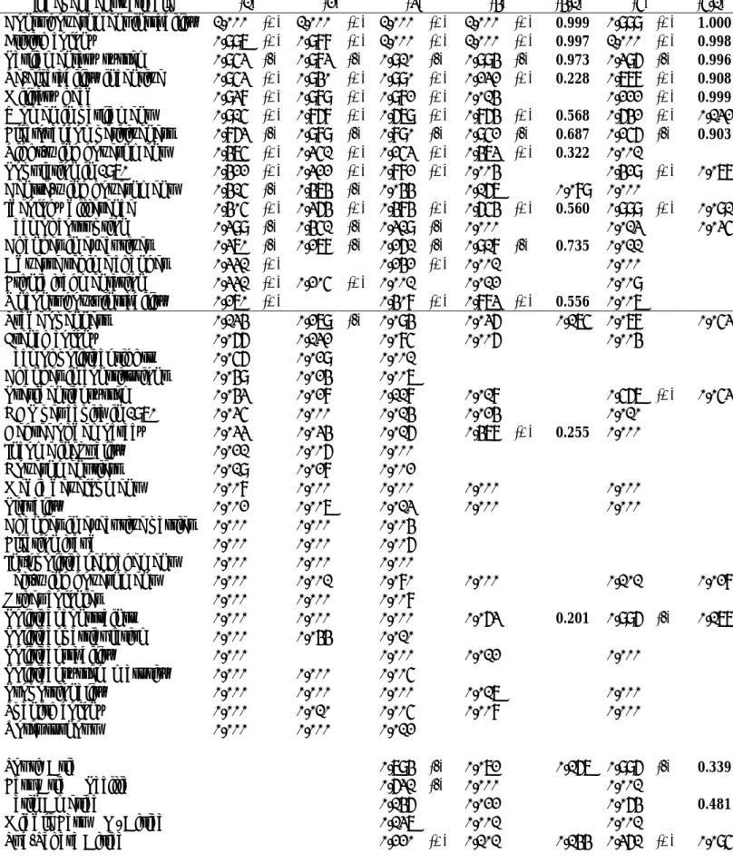
This section shows how the new composite policy volatility indicators are derived. Recall that I construct the policy volatility indicators by applying a principal components analysis (PCA) to a set of the Washington Consensus policy variables. The emphasis will be on the results obtained from a robust PCA rather than a classical PCA.I begin by including all policy variables into a single model, as shown in column (1) of Table 2. The results are promising. Apart fromV DEF ICIT, all other policy variables have an expected, positive correlation with the
Þrst principal component (PC), which explains over 25 percent of the total variance in the data. This however leaves us with only 37 countries.
Column (2) then drops the variables which are available for a limited number of countries. The results reveal that three out ofÞve policy variables which are the development elements of the Consensus (V M DU T Y,V SW,
V SOEF I,V REGF I andV P ROP F I)are more correlated with the second PC than theÞrst PC. Although this cannot be interpreted as a clear-cut ev-idence, it seems to suggest that there are at least two dimensions of policy volatility. More speciÞcally, while the Þrst PC seems to represent macro-economic policy volatility, the second PC appears to capture development policy volatility. It is therefore more sensible to measure them separately.21 Table 3 presents the results for the macroeconomic elements. Column (1) includes all policy variables, and shows that they all have an expected correlation of the expected sign (positive) with the Þrst PC. In column (2) I exclude V DEBT and V M ART AX to increase the sample size, and
V EDU and V HEALT H as they tend to represent the volatility of social policy while the focus is on macroeconomic policy. IÞnd thatV DEF ICIT
virtually has no relationship with theÞrst PC while all other variables are highly correlated with the Þrst PC with the correct sign.22 This justiÞes classifyingV DEF ICIT as one distinct dimension of policy volatility, and
2 1Intuitively, these two types of policy are different. While macroeconomic policy
volatil-ity reßects the lack of government ability in maintaining macroeconomic stability, volatile development policy in general results from policy shifts or liberalization programmes. I discuss this argument later in more detail.
2 2
The results remain unchanged if we drop onlyV DEBTandV M ART AXfrom column (1).
I will refer to it as aÞscal policy volatility indicator.
Recall that V DEF ICIT is the natural logarithm of the standard de-viation of government budget deÞcits over GDP. I test the correctness of this functional form by applying a Box-Cox regression to the standard deviation of budget deÞcits over GDP (V DEF ICIT N L). For our pur-pose, the Box-Cox regression method is used to Þnd the maximum likeli-hood estimate of the parameter θ of the Box-Cox transform, deÞned as:
y(θ) = yθθ−1. The model that I estimate takes this form: V DEF ICIT N Lθ θ−1 =
β1x1j+β2x2j+...+βkxkj+Qj where x’s are the independent variables.23
The results suggest that the value ofθ of zero cannot be rejected, and y(θ)
is therefore transformed to ln(y). This conÞrms that taking the natural logarithm transformation is appropriate.
Column (3) proceeds with the rest of the four macroeconomic policy vari-ables. The preferred model is column (4) where I dropV REALI because, in our sample of developing countries where average inßation rates are high and hyperinßation episodes are not uncommon, movements in the real interest rate depend signiÞcantly on the movements of the inßation rate. Including
V REALI in the analysis could potentially hide the effects of V IN F LA. The robust macroeconomic policy volatility indicator,RV M ACRO, there-fore consists of three variables, and can be written as:
RV M ACRO = 0.220∗V IN F LA0+ 0.786∗V BM P0 (7)
+0.577∗V OV ERV ALU0
where the0 on the policy variables indicates that each has been centred using a robust estimate of their location. The component loadings or weights are comparable across variables, as they are derived from the correlation ma-trix. A higherRV M ACROvalue indicates a more volatile macroeconomic policy.
2 3I obtained these independent variables by performing BMA exercises similar to those
in Table 6. The explanatory variables that form the best model (model with the highest PMP value) include the degree of democracy, presidential system, right-wing government, military head, corruption, trade openness, East Asia dummy, Latin America dummy, land area, and latitude.
It should be noted that the decision to drop V REALI in column (3) and the use of robust rather than classical scores in column (4) are unlikely to affect the results in a meaningful way.24 According to this measure, the
topÞve countries with most stable macroeconomic conditions during 1970-1999 were Singapore, Tunisia, Thailand, Malaysia and Cyprus. In contrast, Democratic Republic of Congo, Ghana, Peru, Uganda and Iran seemed to suffer most from unstable policy.
An alternative measure toRV M ACROis an indicator that assigns equal weights to all policy variables. To construct this, I Þrst apply the Box-Cox regression to the geometric average of the standard deviations of the inßation rate, black market premium and the overvaluation index(V M ACROGA).25
The results again suggest the natural logarithm transformation, which yields
LN V M ACROGAand can be written as:
LN V M ACROGA = 1/3∗V IN F LA+ 1/3∗V BM P (8)
+1/3∗V OV ERV ALU
Recall that V IN F LA,V BM P and V OV ERV ALU are in the natural logarithm form. The differences betweenRV M ACROandLN V M ACROGA
are therefore the weights and that the policy variables which formRV M ACRO
are centred. Despite these differences, the simple correlation between the two indicators is very high (0.95). Even though they are highly correlated, the preferred indicator isRV M ACRObecause the weights are derived more systematically rather than imposed.
2 4
The simple correlation between RV M ACRO and the robust scores obtained from column (3) with four policy variables is 0.96. The macroeconomic volatility indicator from the classical scores,V M ACRO, from column (4) can be written as: V M ACRO= 0.519∗V IN F LA+ 0.609∗V BM P+ 0.600∗V OV ERV ALU. The correlation between
RV M ACROandV M ACROis 0.98.
2 5
V M ACROGA= stdev(inßation rate)1/3 × stdev(black market premium)1/3 ×
stdev(overvaluation index)1/3. I use the geometric average instead of an arithmetic aver-age to reduce the effects of measurement errors and outlying observations. The model I estimate is V M ACROGAθ−1
θ =β1x1j+β2x2j+...+βkxkj+Ajwherex’s are the independent
variables. The independent variables in the best model include political contraints, po-litical stability, constitutional government instability, presidential system, election fraud, government tiers, real GDP per capita in 1970, British colony, French colony, East Asia dummy, South Asia dummy, state antiquity, landlocked country dummy, and latitude.
Finally, Table 4 presents the results for the development elements. In column (2), most policy variables have higher correlations with theÞrst PC with the correct sign. The Þrst PC explains over 31 percent of the total variance in the data. The robust development policy indicator, RV DEV, can be expressed as:
RV DEV = 0.074∗V M DU T Y0+ 0.778∗V SW0+ 0.375 (9) ∗V SOEF I0+ 0.301∗V REGF I0+ 0.397∗V P ROP F I0
A higher RV DEV value indicates a more volatile development policy. The topÞve countries with the most stable development policy during 1970-1999 were Chad, Burundi, Algeria, Mauritius and China. In contrast, Chile, Peru, Bolivia, Turkey and Argentina experienced the least stable policy. As in the case of macroeconomic policy, the use of robust rather than classical scores is unlikely to affect the results.26 It is however not sensible to apply the Box-Cox regression to the geometric average of the standard deviations of development policy variables (V DEV GA) because the values of V SW
and V SOEF I are zero for many countries.
In summary, the three main policy volatility indicators areV DEF ICIT,
RV M ACROandRV DEV. These indicators are available for 87, 72 and 65 developing countries, respectively. As a preliminary test, IÞnd that all three indicators have a negative relationship with the GDP growth rate during 1970-1999, although only the correlation between growth andRV M ACRO
(-0.48) is signiÞcant at the 5 percent level. The next section provides a more systematic regression analysis.
6
Policy Volatility and Growth Regressions
This section empirically tests the growth effects of the three policy volatil-ity indicators. The growth regression speciÞcation that I use is based on Mankiw, Romer, and Weil (1992). The growth rate is deÞned as the log
2 6
The simple correlation betweenRV DEV and the indicator obtained from a classical PCA in column (2), V DEV, is 0.93. V DEV = 0.187∗V M DU T Y + 0.407∗V SW + 0.420∗V SOEF I+ 0.572∗V REGF I+ 0.544∗V P ROP F I
difference in GDP per capita between 1970 and 1999. The explanatory vari-ables include the log of GDP per capita in 1970, the log of the investment share in GDP, the log of population growth adjusted by the capital depreci-ation rate (0.05), a measure of educdepreci-ational attainment in 1970, and regional dummies.
Column (1) in Table 5 shows that, without any other explanatory vari-ables,RV M ACRO has a negative relationship with growth and this is sig-niÞcant at the 1 percent level. RVMACRO alone can explain over 23 per-cent of the total variation in growth rates. Column (2) adds the standard growth determinants while column (3) further adds the regional dummies.
RV M ACRO remains signiÞcant at the 5 percent level. The size of the as-sociation is sizeable. In column (3), a one-standard-deviation decrease in
RV M ACRO (from Senegal to Thailand’s level) raises growth by 0.63 per-centage points. Over the 30-year period, this means a 20 percent increase in the income per capita level.
In column (4), I exclude the investment variable, and show that the size of the growth effect of RV M ACRO increases. This implies that the volatility of macroeconomic policy partly reduces growth by reducing the level of investment.
Columns (5)-(8) test whether volatile macroeconomic policy reduces growth directly or only because it reßects the poor quality of institutions. My main proxy for the quality of institutions is the political constraints variable (P OLCON). First, column (5) shows thatP OLCON has an ex-pected, positive relationship with growth. Importantly, columns (6) and (7) reveal that RV M ACRO remains negatively associated with growth at the 5 percent level after controlling for the effect of institutions. Column (8) conÞrms thisÞnding when an additional three institutional variables are also included. This result is consistent with Fatás and Mihov (2005) who use government consumption as a macroeconomic policy indicator.
These results are not sensitive to the deletion of outlying observations, as detected by median or least absolute deviation (LAD) regression27, DFIT,
2 7
Outlying observations are deÞned as countries whose residuals are greater (less) than the mean value of all residuals plus (minus) two times standard deviation of that country’s residual.
DFBETA, and added-variable plots.28 Diagnostic tests do not indicate any
problems with omitted structure and functional form (from Ramsey’s regres-sion speciÞcation error test) and heteroskedasticity (from the Breusch-Pagan and White tests).
Despite having an expected, negative sign, V DEF ICIT and RV DEV
do not seem to have a link with growth. This Þnding is not sensitive to dropping outliers and dividing the sample into groups of countries with high and low policy volatility. The absence of a budget deÞcit volatility and growth relationship is also found in Aizenman and Marion (1993).29 The limited role of development policy casts more surprise, as it might be expected that unstable policy such as unpredictable government regulations would discourage investment and growth. A closer look at the data reveals that many countries with highly volatile development policy are those that implemented liberalization programmes (such as Chile, Peru and Argentina). In contrast, many countries with very stable policy are in fact those that appear to have persisted in poor policy (such as Burundi and Chad).30
In addition to output growth, I also tested the relationship between the policy volatility indicators and the shares of total and private investment in output during 1970-1999. The results are less promising than the growth regression Þndings. The regional dummies seem to play a great role here. For example, the analysis shows that RV M ACRO reduces total and pri-vate investment andRV DEV reduces total investment only when regional dummies are not included.31
2 8
The results are available upon request. Cook and Uchida (2003, pp. 153-54) brießy explain how DFITS and DFBETA are computed and used.
2 9
The stylized fact in Table 1 also shows that while the difference in output growth rates between high and low-income countries is sizeable, low-income countries are not subject to much higher budget deÞcits. It is important to note that most studies which document a negative link betweenÞscal policy volatility and growth use central government consump-tion as a proxy. This paper uses government budget deÞcits because my main objective is to explain a government’s ability to maintain macroeconomic stability, not the use of discretion in implementing policy.
3 0
For example, the average value of the Sachs and Warner (1995) index during 1970-1999 for the topÞve countries with the most (least) volatile development policy is 0.51 (0.20). This means that the topÞve countries with the most volatile policy are considered as open economies in about 15 out of 30 years while the corresponding statistic is only 6 years for countries with stable policy.
7
Explaining Policy Volatility
In the last section, we saw that only macroeconomic policy volatility has an explanatory power for growth. The rest of this paper will therefore investigate the factors that explain the variation in RV M ACRO. It Þrst uses a Bayesian model averaging (BMA) approach to evaluate sets of possible independent variables. Section 7.2 then uses the sets of variables that are suggested by BMA to estimate regressions that explain the causes of policy volatility.
7.1
BMA Results
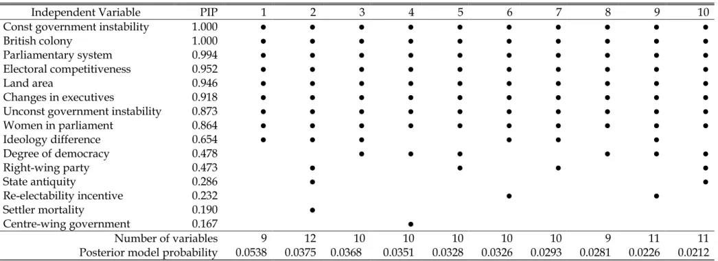
This section describes how a BMA exercise is performed and suggests two lists of explanatory variables that form the best models from two different samples. I start in column (1) of Table 6 by including 39 main independent variables. These are political and social variables, which tend to have a clearer interpretation as to how they affect policy volatility than variables such as pre-determined factors. Only variables with a posterior inclusion probability (PIP) value of 0.20 and over are considered important. The
Þrst column suggests 16 of these variables, while (+) and (-) indicate the directions of relationship between that variable and RV M ACRO.32 These results are not sensitive to various alternative proxies.33
3 2In another experiment, I also included some variables which have a less clear
inter-pretation than these 39 main variables such as special interests of the executive party (nationalist and regional-oriented) and the shares of population with different religions. These variables however have low PIP values.
3 3
This includes (1) replaceP OLIT Y with the degree of democracy variables from Reich (2002,REICEDEM) and Golder (2004,GOLDERDE). (2) Replace P OLST AB with
N V U N REST, V IU N REST, and three indicators of socio-political instability by Vu Le (2001,V U LESP I,V U LESP I1and V U LESP I2). (3) ReplaceP OLCON with the number of government seats over total seats (M AJ ORIT Y), the HerÞndahl index of government seat shares (HERF GOV), the chance that two deputies randomly selected will be from different parties (GOV F RAC), a dummy indicating whether the party of executives controls all houses that have lawmaking powers (ALLHOU SE), the score that measures the strength of checks and balances system (CHECKS), and the proportion of veto players who drop from the government (ST ABS). All these variables are from Beck et al. (2001). I also tried the executive constraints variable from Marshall and Jaggers (2002,XCON ST). (4) ReplaceM EDIADEV with an index of press freedom by Karlekar (2004,F REEP RES). (5) ReplaceF RU ADELEwith the score of free and fair elections by Coppedge and Reinicke (1990,P OLY ARC) and a variable that measures the universal
One can imagine that in countries where political violence is common, the mechanisms by which these main variables inßuence policy volatility might be different from countries where social order is maintained. An in-clusion of variables which measure severe disorder might therefore bias the results of other variables. To test this argument, column (2) drops three variables including adverse regime changes (ADREGCHG), the probabil-ity of unlawful changes in the government (P ROBIRCH), and political stability (P OLST AB). The results in column (1) do not seem to change signiÞcantly.34
Column (3) adds Þve regional dummies while column (4) adds four his-torical variables and eight geographic variables into column (2).35 Among
others, column (4) suggests that macroeconomic policy is more stable in countries where government instability is low, elections are more competi-tive, the difference in the political ideologies among political parties is small, and the executive party follows a liberal ideology. In addition, countries which are more democratic, are former British colonies, and adopt parlia-mentary system tend to have more stable macroeconomic policy.
Finally, column (5) drops the settler mortality variable (M ORT AL) from column (4) because it is available for a lower number of countries. In total, column (5), which is the preferred set of results, suggests 14 variables with PIPs over 0.20. Among others, it reveals that while adopting a presidential system tends to raise policy volatility, stronger political contraints help to reduce policy volatility.
Table 7 displays the structure of the top ten models, ranked by their posterior model probability (PMP) values, from column (5) of Table 6. It shows that the best model consists of ten variables. These variables will application of the right of voting by Paxton et al. (2003, SU F F RAGE). The only unrobust case is when we replace ethnic fragmentation (ET HN F RAC) with linguistic (LIN GF RAC) and religious fragmentation (RELIF RAC). UnlikeET HN F RAC, the PIP values ofLIN GF RACandRELIF RACare lower than 0.20, and the results of other variables remain largely the same.
3 4This Þnding remains unchanged when dropping only ADREGCHG and
P ROBIRCH, which have the PIP values over 0.20 in column (1).
3 5
Although thebicregsoftware for R can handle up to 49 variables in a single model, the maximum number of variables I use is 45 variables to allow for a manageable computation time. As a result, I drop 11 variables in column (4). These are the variables with low PIP values in column (3).
form the baseline model in the next section. The PMP value of the best model is 0.04, compared with the prior probability, considering that there are 244 possible models to estimate, of 5.7× 10⁻¹⁴. Table 8 displays the
top ten models from column (4) of Table 6.
Overall, it can be argued that the results are not excessively fragile. Those variables with very high PIP values in column (1) remain impor-tant across all experiments. It is also shown that electoral rules and media development do not seem to inßuence policy volatility. In addition, while historical and geographic variables appear to inßuence the results in column (5), they themselves have limited explanatory power.
To check the robustness of these results from the bicreg approach, I applied aM C3 approach to columns (4) and (5). The results are shown in
columns (4.1) and (5.1). An important software limitation here is that the number of variables that can be included in a M C3 exercise must not be
greater than half of the number of observations. Hence, in column (4.1), only the top 20 variables with the highest PIP values in column (4) are included. In column (5.1), they are the top 25 variables from column (5). Similar to thebicreg case, the variables with the posterior probabilities of 0.20 or greater are considered important and are in bold.
Column (4.1) shows that out of 13 variables that have PIP values greater than 0.20 in column (4), 12 of these variables are also suggested by aM C3
approach. The results are less strong in column (5.1) where eight (out of 15) variables are emphasized by both approaches. It can however be seen that results for the variables with high PIPs value are robust. Overall, these robustness results are promising, considering that columns (4) and (5) have many more variables than columns (4.1) and (5.1). This suggests that the results from thebicreg appraoch are not excessively inßuenced by outlying observations.
7.2
Regression Results
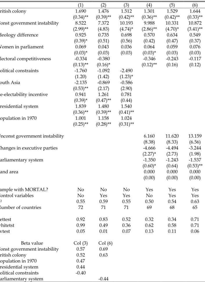
This section uses a simple regression analysis to study the roles of the vari-ables in the best models in Tvari-ables 7 and 8 in explainingRV M ACRO.
in Table 7 (the sample that excludes M ORT AL). It shows that nearly all variables have a signiÞcant relationship withRV M ACRO at the 5 percent level. Taken together, these variables explain over half the total variation in the data. Column (2) adds the initial income level and regional dummies as control variables. It suggests that macroeconomic policy is more volatile in countries that adopt a presidential system and where electoral outcomes are less competitive. Countries which are former British colonies and have larger populations also experience less stable policy.
Note that the political constraints variable (P OLCON) is the only vari-able that is not signiÞcant in column (1). The reason might be that the electoral competitiveness variable (LIEC) hides the effect of P OLCON
since both variables proxy for government power in implementing discre-tionary policy (the simple correlation is 0.71). Column (3) therefore drops
LIEC and reveals that stronger constraints in the policy-making process do lower policy volatility.36 It also shows that macroeconomic policy is less volatile when the chance that the government in power will be replaced (via constitutional means) (P ROBM JCH) is lower. These results are robust to the deletion of outlying observations as detected by the median regression method.
Column (4) contains nine variables that form the best model in Table 8 (the sample that includesM ORT AL). Five of these variables also appear in the best model in the sample withoutM ORT AL. The overall results remain unchanged, i.e. government instability, less competitive electoral outcomes, and being a former British colony increase policy volatility. Column (5) adds control variables and somewhat weakens the Þndings in column (4).
The results in column (5) are not sensitive to excluding three outliers as suggested by the median regression method (Iran, Guatemala, and the Democratic Republic of Congo) as shown in column (6). An exception is the relationship betweenRV M ACROand a parliamentary system (P ARLIA) which became signiÞcantly negative at the 1 percent level. That is, parlia-mentary regimes are associated with more stable policy.
The sizes of association between these explanatory variables and
macro-3 6Between the two variables,P OLCON is preferred since it appears in all ten models
economic policy volatility are displayed at the bottom panel of Table 9 (only the variables that are signiÞcant at the 5 percent level in columns (3) and (6) are shown). The beta value indicates the size of the change inRV M ACRO
(in terms of its standard deviation) given a one-standard-deviation change in the independent variable. For example, based on the estimates in column (3), a one-standard-deviation increase inP ROBM JCH (from Thailand to Chile’s level) raisesRV M ACROby 0.57 of a standard deviation (from Thai-land to Jordan’s level).
One general conclusion that can be drawn from this section is that while a presidential regime leads to a more volatile policy, stronger political con-straints help to stabilize policy. This is true when we measure policy volatil-ity both in terms of inßation and real exchange rates as in this paper, and in term of government spending as in Fatás and Mihov (2003). Moreover, while the literature has highlighted the important role of trade openness in explaining the volatility of inßation and real exchange rates, this paper documents that once we control for a wider range of independent variables, the explanatory power of trade openness seems to disappear.
8
Conclusions
This paper has sought to explain the causes of government policy volatility in developing countries. To measure policy volatility, I applied a method of classical and outlier-robust principal components to the proxies of Wash-ington Consensus policy variables. The results suggest three dimensions of policy volatility, namely, Þscal, macroeconomic and development policy volatility.
I showed that more volatile macroeconomic policy is associated with lower income per capita growth even after controlling for the proxies for the quality of institutions. The size of the association is notable. In the preferred model, a one-standard-deviation decrease in the composite macroeconomic policy volatility indicator raises growth by 0.63 percentage points. It is also shown that changes in development or liberalization policy and unstable
Þscal deÞcits do not appear to affect economic growth.
uncer-tainty problem. The key Þndings are that macroeconomic policy is more volatile in countries that adopt a presidential system, have weaker politi-cal constraints, and where government stability is lower. Countries which are former British colonies and have larger populations also experience less stable policy. Finally, adopting a parliamentary regime seems to help to stabilize policy. A one-standard-deviation change in these variables results in a 0.40-0.57 standard deviation change in the policy volatility indicator.
Two important issues arise from these Þndings. First, it is arguable that macroeconomic instability can also inßuence the strength of political constraints (e.g. through changes in legislature) and the degree of govern-ment stability. The next empirical task is therefore to study the casual relationships between these two variables and macroeconomic stability. Sec-ond, we saw that the type of political regime (presidential and parliamen-tary) plays an important role in explaining policy volatility in developing countries. While theoretical work which attempts to explain how political regimes affect policy outcomes is growing rapidly (see for example Persson and Tabellini, 2003), much of this work focuses on democratic countries. An ability to explain how political regimes and policy outcomes interact in less democratic contexts remains a challenge.
References
[1] Acemoglu, Daron, Simon Johnson and James Robinson (2001), “The colonial origins of comparative development: An empirical investiga-tion”, American Economic Review, 91, 1369-1401.
[2] Acemoglu, Daron, Simon Johnson, James Robinson and Yunyong Thaicharoen (2003), “Institutional causes, macroeconomic symptoms: Volatility, crises and growth”, Journal of Monetary Economics, 50, 49-123.
[3] Agénor, Pierre-Richard (2004), “Macroeconomic adjustment and the poor: Analytical issues and cross-country evidence”, Journal of Eco-nomic Surveys, 18, 351-408.
[4] Aizenman, Joshua and Nancy Marion (1993), “Policy uncertainty, per-sistence and growth”, Review of International Economics, 1, 145-163. [5] Aizenman, Joshua and Nancy Marion (1999), “Volatility and
invest-ment: Interpreting evidence from developing countries”, Economica, 66, 157-179.
[6] Alesina, Alberto, Arnaud Devleeschauwer, William Easterly, Sergio Kurlat and Romain Wacziarg (2003), “Fractionalization”, Journal of Economic Growth, 8, 155-79.
[7] Ali, Abdiweli and Hodan Said Isse (2004), “Political freedom and the stability of economic policy”,Cato Journal, 24, 251-260.
[8] Anbarci, Nejat, Jonathan Hill and Hasan Kirmanoglu (2005), “Institu-tions and growth volatility”, Mimeo,
[9] Barro, Robert and Jong-Wha Lee (2000), “International data on educa-tional attainment: Updates and implications”, NBER Working Paper No.7911, National Bureau of Economic Research, Cambridge.
[10] Beck, Thorsten, George Clarke, Alberto Groff, Philip Keefer, and Patrick Walsh (2001), “New tools in comparative political economy: The Database of political institutions”,World Bank Economic Review, 15, 165-176.
[11] Bleaney, Michael (1996), “Macroeconomic stability, investment and growth in developing countries”, Journal of Development Economics, 48, 461-477.
[12] Bleaney, Michael and David Greenaway (2001), “The impact of terms of trade and real exchange rate volatility on investment and growth in sub-Saharan Africa”, Journal of Development Economics, 65, 491-500. [13] Bockstette, Valerie, Areendam Chanda and Louis Putterman (2002), “States and markets: The advantage of an early start”, Journal of Economic Growth, 7, 347-369.
[14] Bowdler, Christopher and Adeel Malik (2005), “Openness and inßation volatility: Panel data evidence”, Mimeo.
[15] Bravo-Oetega, Claudio and Julian di Giovanni (2005), “Remoteness and real exchange rate volatility”, IMF Working Paper No.WP/05/01, International Monetary Fund, Washington D.C.
[16] Breen, Richard and Cecilia García-Peñalosa (2005), “Income inequality and macroeconomic volatility: An empirical investigation”, Review of Development Economics, 9, 380-398.
[17] Brunetti, Aymo (1998), “Policy volatility and economic growth: A com-parative, empirical analysis”, European Journal of Political Economy, 14, 35-52.
[18] Brunetti, Aymo, Gregory Kisunko and Beatraice Weder (1998), “Cred-ibility of rules and economic growth: Evidence from a worldwide survey of the private sector”,World Bank Economic Review, 12, 353-384. [19] Brunetti, Aymo and Beatraice Weder (1998), “Investment and
institu-tional uncertainty: A comparative study of different uncertainty mea-sures”,Weltwirtschaftliches Archiv, 134, 513-533.
[20] Calderón, César (2004), “Trade openness and real exchange rate volatil-ity: Panel data evidence”, Working Paper No.294, Central Bank of Chile.
[21] Cook, Paul and Yuchiro Uchida (2003), “Privatisation and economic growth in developing countries”, Journal of Development Studies, 39, 121-154.
[22] Coppedge, Michael and Wolfgang Reinicke (1990), “Measuring pol-yarchy”,Studies in Comparative International Development, 25, 51-72. [23] Dawson, John (2005), “Regulation, investment, and growth across
countries”, Mimeo, Appalachian State University.
[24] De Mesquita, Bruce, Alastair Smith, Randolph Siverson and James Morrow (2003), The Logic of Political Survival,
The MIT Press, Massachusetts. Data sets are available at http://www.nyu.edu/gsas/dept/politics/data/bdm2s2/Logic.htm [25] Dixit, Avinash and Robert Pindyck (1994), Investment Under
Uncer-tainty, Princeton University Press, New Jersey.
[26] Dollar, David (1992), “Outward-oriented developing economies really do grow more rapidly: Evidence from 95 LDCs, 1976-1985”, Economic Development and Cultural Change; 40(3), 523-544.
[27] Dollar, David and Aart Kraay (2002), “Growth is good for the poor”,
Journal of Economic Growth, 7(3), 195-225.
[28] Dreher, Axel (2003), “Does globalization affect growth?”, Mimeo, Uni-versity of Mannheim.
[29] Dutt, Pushan and Devashish Mitra (2004), “Inequality and the insta-bility of polity and policy”, Mimeo.
[30] Easterly, William (2005), “National policies and economic growth: A reappraisal” in Philippe Aghion and Steven Durlauf (eds.)Handbook of Economic Growth, North-Holland, 1015-1059.
[31] Easterly, William, Roumeen Islam and Joseph Stiglitz (2000), “Shaken and Stirred: Explaining Growth Volatility” in Boris Pleskovic and Nicholas Stern (eds.)Annual World Bank Conference on Development Economics, World Bank, Washington D.C.
[32] Easterly, William and Mirvat Sewadeh (2002), Global Development Network Growth Database, World Bank. http://www.worldbank.org/research/growth/GDNdata.htm
[33] Elbadawi, Ibrahim and Klaus Schmidt-Hebbel (1998), “Macroeconomic policies, instability and growth in the world”, Journal of African Economies, 7, 116-168.
[34] Falvey, Rod and Norman Gemmell (1999), “Factor endowments, non-tradables prices and measures of openness”, Journal of Development Economics, 58, 101-122.
[35] Fatás, Antonio and Ilian Mihov (2003), “The case for restrictingÞscal policy discretion”, Quarterly Journal of Economics, 118, 1419-1447. [36] Fatás, Antonio and Ilian Mihov (2004), “Fiscal discipline, volatility and
growth”, Mimeo.
[37] Fatás, Antonio and Ilian Mihov (2005), “Policy volatility, institutions and economic growth”, Mimeo.
[38] Feng, Yi (1997), “Democracy, political stability and economic growth”,
British Journal of Political Science, 27, 391-418.
[39] Feng, Yi, Jacek Kugler and Paul Zak (2000), “The politics of fertility and economic development”, International Studies Quarterly, 44, 667-693.
[40] Fischer, Stanley (2003), “Globalization and its challenges”, American Economic Review, 93, 1-30.
[41] Furnival, George and Robert Wilson Jr. (1974), “Regression by leaps and bounds”, Technometrics, 16, 499-511.
[42] Gallup, John, Jeffrey Sachs with Andrew Mellinger (1999), “Geogra-phy and economic development” in Boris Pleskovic and Joseph Stiglitz (eds.) Annual World Bank Conference on Development Economics, World Bank, Washington D.C.
[43] Golder, Matt (2005), “Democratic electoral systems around the world, 1946-2000”,Electoral Studies, 24(1), 103-121.
[44] Gwartney, James and Robert Lawson (2004),Economic Freedom of the World: 2004 Annual Report, The Fraser Institute, Vancouver.
[45] Hall, Robert and Charles Jones (1999), “Why do some countries pro-duce so much more output per worker than others?”,Quarterly Journal of Economics, 114, 83-116.
[46] Hau, Harald (2002), “Real exchange rate volatility and economic open-ness: Theory and evidence”, Journal of Money, Credit, and Banking, 34, 611-630.
[47] Haveman, Jon, “Empirical investigations in international trade” web-site (www.eiit.org).
[48] Henisz, Witold (2000), “The institutional environment for economic growth”, Economics and Politics, 12, 1-31.
[49] Henisz, Witold (2004), “Political institutions and policy volatility”,
Economics and Politics, 16, 1-27.
[50] Heston, Alan, Robert Summers and Bettina Aten (2002), Penn World Table Version 6.1, Center for International Comparisons, University of Pennsylvania.
[51] Hnatkovska, Viktoria and Norman Loayza (2004), “Volatility and growth”, World Bank Policy Research Working Paper No.3184, World Bank, Washington D.C.
[5