Computer Science and Engineering: Theses,
Dissertations, and Student Research Computer Science and Engineering, Department of
12-2018
Scale-Out Algorithm For Apache Storm In SaaS
Environment
Ravi Kiran Puttaswamy
University of Nebraska-Lincoln, [email protected]
Follow this and additional works at:http://digitalcommons.unl.edu/computerscidiss Part of theComputer Engineering Commons, and theComputer Sciences Commons
This Article is brought to you for free and open access by the Computer Science and Engineering, Department of at DigitalCommons@University of Nebraska - Lincoln. It has been accepted for inclusion in Computer Science and Engineering: Theses, Dissertations, and Student Research by an authorized administrator of DigitalCommons@University of Nebraska - Lincoln.
Puttaswamy, Ravi Kiran, "Scale-Out Algorithm For Apache Storm In SaaS Environment" (2018).Computer Science and Engineering: Theses, Dissertations, and Student Research. 159.
by
Ravi Kiran Puttaswamy
A THESIS
Presented to the Faculty of
The Graduate College at the University of Nebraska In Partial Fulfilment of Requirements
For the Degree of Master of Science
Major: Computer Science
Under the Supervision of Ying Lu
Lincoln, Nebraska December, 2018
Ravi Kiran Puttaswamy, M.S. University of Nebraska, 2018 Adviser: Ying Lu
The main appeal of the Cloud is in its cost effective and flexible access to computing power. Apache Storm is a data processing framework used to process streaming data. In our work we explore the possibility of offering Apache Storm as a software service. Further, we take advantage of the cgroups feature in Storm to divide the computing power of worker machine into smaller units to be offered to users. We predict that the compute bounds placed on the cgroups could be used to approximate the state of the workflow. We discuss the limitations of the current schedulers in facilitating this type of approximation as the resources are distributed in arbitrary ways. We implement a new custom scheduler that allows the user with more explicit control over the way resources are distributed to components in the workflow. We further build a simple model to approximate the current state and also predict the future state of the workflow due to changes in resource allocation. We propose a scale-out algorithm to increase the
throughput of the workflow. We use the predictive model to measure the effects of many candidate allocations before choosing it. Our approach analyzes the strengths and drawbacks of Stela algorithm and design a complementary algorithm. We show that the combined algorithm complement each others strengths and drawbacks and provides allocations to maximize throughput for much larger set of scenarios. We implement the algorithm as a stand alone scheduler and evaluate the strategy through physical
simulation on the Apache Storm Cluster and on software simulations for a set of workflows.
COPYRIGHT
ACKNOWLEDGMENTS
Foremost, I would like to express my sincere gratitude to my advisor Prof. Ying Lu for the continuous support of my study and research, for her patience, motivation, enthusiasm, and immense knowledge. Her guidance helped me in all the time of research and writing of this thesis. I could not have imagined having a better advisor and mentor for my Masters Thesis.
Besides my advisor, I would like to thank the rest of my thesis committee: Prof. David Swanson and Prof. Hongfeng Yu, for their encouragement and insightful comments.
I would also like to thank the CSE department and HCC for providing ample amount of support and resources to help me complete my work.
Finally I would like to my family and friends, without whom I wouldn’t be here today.
Contents
List of Figures vii
List of Tables ix
1: Introduction 1
2: Literature Review 8
3: Background 16
3.1 Architecture of Apache Storm . . . 18
4: Stela 24 4.1 Identify Congested Components . . . 25
4.2 Measure Desirability of Congested Component . . . 25
4.3 Choosing The Component . . . 26
4.4 Drawbacks of Stela . . . 27
5: Scale-Out Algorithm 29 5.1 Goals and Assumptions . . . 29
5.2 Approach and Design. . . 30
5.2.1 Resource Units . . . 31
5.2.2 Batch Allocation . . . 31
5.2.4 Calculating Throughput for Allocation . . . 34
5.2.5 Strategy. . . 35
5.2.6 Residual Resources. . . 37
5.2.7 Algorithm. . . 38
5.2.8 Comparision to Stela. . . 42
6: Implementation and Evaluation 45 6.1 Changes to Storm Framework . . . 46
6.2 Evaluation . . . 47 6.2.1 Software Simulation . . . 48 6.2.2 Analysis . . . 59 6.2.3 Validation in Testbed . . . 63 7: Future Work 70 8: Conclusion 72 References 73
List of Figures
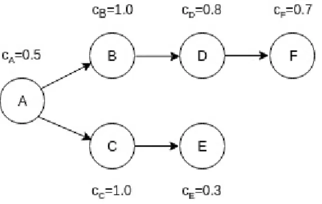
1.1 A sample topology where Cx indicates the level of congestion. It varies
be-tween 0 (no congestion) and 1.0 (fully Congested) . . . 4
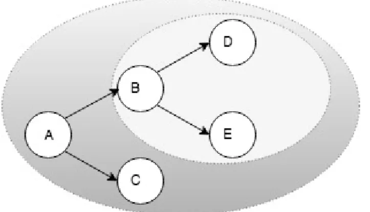
1.2 A sample topology with more components. Cxindicates the level of conges-tion. It varies between 0 (no congestion) and 1.0 (fully Congested) . . . 4
1.3 Tree structure of the topology. For the entire topology A is the rootnode. B,D,E,C are the children. B,E,D is a child subtree of A. B is the root of the subtree 6 3.1 Topology structure indicating Spout and Bolt . . . 17
3.2 High Level Architecture of Apache Storm . . . 18
3.3 Architecture of Worker Process1 . . . . 19
3.4 Task distribution in a Topology . . . 20
3.5 Internal message buffer of worker process . . . 22
6.1 Test topology : linear . . . 50
6.2 Test topology : Diamond . . . 51
6.3 Test topology : simple Tree . . . 52
6.4 Test topology : topology 17 . . . 54
6.5 Throughput increase comparison for Test topology : topology 17 . . . 55
6.6 Throughput increase comparison for topology 17 with child ratios swapped . 56 6.7 Throughput increase comparison for topology 17 step capacity increased . . . 57
6.8 Throughput increase comparison for topology 17 step capacity increased child
ratio swapped . . . 58
6.9 Test topology : testMix topology . . . 59
6.10 Throughput increase comparison for testMix topology . . . 59
6.11 Throughput increase comparison for testMix with child ratio swapped : test-MixRev topology . . . 61
6.12 Throughput increase comparison for testMix with step capacity increase : testMixStep topology . . . 61
6.13 Throughput increase comparison for testMix with step capacity increase and child ratio swapped : testMixStepRev topology . . . 62
6.14 Throughput increase comparison for combined algorithm and Stela . . . 64
6.15 Throughput increase comparison for combined algorithm and Stela . . . 67
6.16 Test topology : topology 10 . . . 68
6.17 Throughput increase comparison Stela and our approach : topology 10 . . . . 68
6.18 Throughput increase comparison Stela and Combined : topology 10 . . . 68
List of Tables
6.1 Input, output and max processing rates for topology : linear . . . 50
6.2 Allocations and throughput increase for topology : linear . . . 50
6.3 Input, output and max processing rates for topology : diamond . . . 51
6.4 Allocations and throughput increase for topology : diamond . . . 51
6.5 Input, output and max processing rates for topology : simple tree. . . 52
6.6 Allocations and throughput increase for topology : simple tree . . . 53
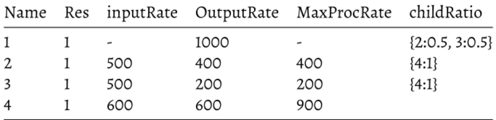
6.7 Input, output and max processing rates for topology : topology 17. . . 53
6.8 Allocations and throughput increase for topology : topology 17 . . . 54
6.9 Input, output and max processing rates for topology : topology 17. . . 56
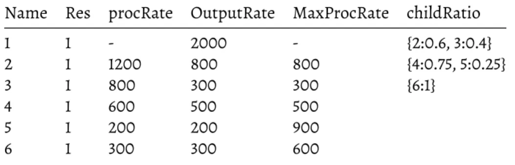
6.10 Input, output and max processing rates for topology : mix topology . . . 60
Chapter 1
Introduction
Cloud computing technology has received widespread acceptance in the recent years. Companies are moving their assets and workloads to the cloud through mixed or pure cloud deployments in ever increasing numbers.2The cloud offers a lot of flexibility by
allowing the user to procure resources on demand, which reduces operational costs. Cloud computing is offered in many flavors, to better suit the user’s perception of the infrastructure. Some of the popular flavors are Infrastructure as a Service (IaaS), Platform as a Service (PaaS) and Software as a Service (Saas). In IaaS, the computing resources and the supporting infrastructure like networking, storage etc. are owned by the cloud providers. The user can procure these resources on demand. This flavor provides the greatest freedom, as the user can customize the infrastructure and the software. PaaS offers the middleware with the infrastructure. Middleware typically includes the operating system, development tools, database management system, etc. The user typically deploys his application using the tools provided by the middleware. SaaS offers a complete software solution as a service. The user can connect to the software and use it over the internet. The applications are deployed and maintained by the cloud provider or a third party agent, and the user has no access or control over the infrastructure that hosts the service.
One of the technologies to take advantage of this form of computing is Big Data. Cloud computing along with the recent advancements to the data processing
frameworks has greatly reduced the barrier of entry to many medium and small sized companies. Apache Hadoop,3Apache Storm,4Apache Spark,5Heron,6Milwheel,7Apache
Zookeeper,8S49are among the more popular frameworks used for big data processing.
Creating and maintaining a data center is expensive and often untenable for small companies. Instead now they can take advantage of the infrastructure provided by the cloud. The cloud and the frameworks enable the user to develop their solutions quickly and test the viability and usefulness of these big data solutions before committing to it fully.
The current approaches to deploy big data applications often obtain resources in either IaaS10or PaaS11flavor. Typically machines are acquired and configured with the
necessary software like data processing framework. These approaches place some burden on the user as they are responsible for deploying, configuring and maintaining the necessary software. For small companies such investments in resources may be untenable. In our work we explore the possibility of offering data processing frameworks in a SaaS flavor.
SaaS has seen steady growth in recent times.12When a software is offered as service,
the service provider installs, configures and maintains the software. The user accesses the software through a service point. The whole infrastructure supporting the software is abstracted and hidden from the user. The user has no control over the machines on which the software is hosted, or on the software itself. The software provider defines the operations that the user can execute as well as the means to acquire or release resources.
For the SaaS flavor of data processing frameworks, the user only needs to provide the workflow to execute and the number of resources to be used. The service provider would allocate the requested resources and execute the topology on the cloud. The user does not have any control over the machines or the software or where the workflow is
deployed. It is up to the service provider to ensure that the workflow is executed in isolation and its performance is not impacted by workflows of other users. Additionally the service provider needs to ensure that the privacy and security concerns of users are addressed. This could be done externally by using containers or internally if the data processing framework supports features similar to containers.
Apache Storm is a popular framework used to process streaming data. This project is open sourced,13in active development and has widespread usage. The workflow for
processing data is called a Topology. A topology is described in the form of an acyclic graph. Each node represents some task to be performed on data and the arcs indicate the flow of data between nodes. Compute resources are allocated to the node to execute the task. The part of the framework responsible for allocating the compute resources to the components is called a Scheduler. Resources are typically allocated at the beginning of the execution of the workflow. The user can add or remove additional resources to accommodate changes in the workload. This operation is called Scaling a topology. This becomes a very important operation in the cloud environment, as the user wants to maintain just as many resources as needed. In our work, we concentrate on adding resources to topology also called the Scale Out operation.
Deciding on which node should receive the resources can be extremely tricky in some cases. Consider the scenario where the user wants to scale the topology by allocating resources to relieve the congested components.
In the topology shown in figure1.1, nodes B and C are congested. Allocating the resource to either B or C seems to be the obvious solution. Allocating the resource to B would decongest the component and increase the output from B. However D and F are already running close to their capacity. It is possible that one or both of them could get congested. The net effect of the allocation would have been to transfer the congestion to a downstream node, resulting in little improvement in throughput. In this case,
Figure 1.1: A sample topology whereCxindicates the level of congestion. It varies between
0 (no congestion) and 1.0 (fully Congested)
and the throughput could depend on many factors. Thus, generating an optimal allocation for a resource is a challenging task.
When multiple resources are provided for allocation, the scheduling problem becomes even more complicated. Consider the following example when two resources are provided for allocation.
Figure 1.2: A sample topology with more components.Cxindicates the level of congestion.
It varies between 0 (no congestion) and 1.0 (fully Congested)
In the sample topology shown in figure1.2nodes B, C and D are congested. Two resources are provided to the scheduler to allocate to the topology. These resources can be allocated to
• the most congested components in the B branch (.i.e. to B and D) • components C and F
• component B and the remaining resource to either C or F
As the number of resources increase, the number of ways the resources can be distributed among the components also increases drastically. Suppose a topology contains ‘n’ number of components and ‘r’ resources are procured for allocation. Each of the resource can be allocated in ‘n’ ways. The total number of possible allocations arenr.
Even if we restrict the allocation to only congested components, during the allocation child components can potentially get congested and will need to be considered for allocation. Thusnrgives the worst case possibilities.
Iterating and evaluating through all the possible distributions can be time consuming. Picking the right solution requires the scheduler to consider a number of factors related to the topology both in current state, and the possible state after allocation. This further illustrates the complexity of scheduling multiple resources.
There are two approaches to allocate multiple resources. One way would be to allocate them in a serial manner. Each instance of the resource is considered in isolation. At any given time, optimal allocation for only one instance is calculated and assigned, before considering the next instance. Such a scheduling strategy is called Serial
allocation. The other way is to consider a set of resources at a time for allocation. The set of resources considered is called a batch. The allocation for all the resources in the batch is calculated at the same time, before considering the next batch. Typically, for small number of resources all the resources are grouped into a single batch. Such a scheduling strategy is called Batch Allocation. A scheduler typically opts for one of these approaches. The relative merits and the trade offs of each of the approaches will be discussed later.
We base our work on a scheduler called Stela.14Stela implements a scaleout
topology by allocating resources to congested nodes. In order to choose between congested nodes, Stela uses a novel method to measure the impact of the nodes on the throughput. If the throughput of the subtree under the congested component is high, then the impact is determined to be high. Stela picks the component with the highest impact, allocates a resource and updates the state of components in the topology. The steps are repeated for each resource. Once the resource is allocated, it is absolute and it cannot be reallocated.
Stela uses a relatively simple approach. Stela prioritizes paths with the highest impact on throughput to decongest. More often than not, this strategy leads to optimal results. Stela assumes correlation between the impact of a congested component to the throughput. This assumption is the main strength as well as a drawback for Stela. Apart from impact, there are other factors that contribute to the throughput like the state of the subtree. If the subtree is already running near capacity, then the allocation just moves the congestion downstream and the throughput increase may be less than expected. In our algorithm, we attempt to address such limitations.
We now define the conventions of how the term "root", "subtree", "children", "child Subtree" are used in our work. The terms are used only to our work.
Figure 1.3: Tree structure of the topology. For the entire topology A is the rootnode. B,D,E,C are the children. B,E,D is a child subtree of A. B is the root of the subtree
B,D,E,C are treated as "children" of A. {B,D,E} is a "subtree" of A. {C} is also a subtree of A. In the subtree {B,D,E}, B is the "root" and {D,E} are the "children". In the work, when B is referred to as the "root", it is done so in the context of the "subtree" with B as the root. The children of the root node refer to all the nodes under the root node, and not just the immediate child nodes unless otherwise specified.
In our work, we look at using the new features developed by Apache Storm to support it in a SaaS flavor. We mainly focus on the scale-out operation of a topology. Given additional compute resources, we provide an effective algorithm to allocate the resources to the components to maximize the throughput of the topology.
Chapter 2
Literature Review
For the literature review, we first examine the role and usage of clusters in the context of private in-house deployment and public clouds. We then consider some of the research efforts related to scheduling which determines allocation of tasks from a workflow to a cluster. Finally we consider related work which focuses on model based scheduling, as we use the same approach in our scaleout algorithm.
Clusters were traditionally used for high performance and high throughput computing, and were often shared among many users or teams. HTCondor15is one of
the oldest software solutions and was initially designed to harness cpu power from idle desktop workstations. User can submit a job to HTCondor. HTCondor then chooses machines from the available pool, executes the job and returns it back to the user. The user can specify some constraints over which machines can execute the job, but it is up to HTCondor to select the right machines.
Borg16is a cluster management software used at Google. Borg is used to execute
production jobs and non-production jobs. Production jobs are very sensitive to latency and are executed with higher priority, while the non-production jobs are treated with lower priority. The cluster is divided into cells, each cell containing thousands of machines running a mix of production and non-production jobs. Jobs from different
users are executed within the same cell and sometimes on same machine. Each job contains a set of tasks. The user can apply some additional constraints to the tasks. When a user submits a job to Borg, Borg looks for machines that match the user defined constraints to schedule the job. In order to improve machine utilization, Borg uses containers to execute the jobs. Every job has a priority assigned to it. Borg allows jobs of lower priority to be preempted by higher priority jobs to ensure that production jobs are not starved of resources. Borg presents a typical view of a cluster management software used in companies. Other companies have similar software used to manage their private clusters17181920and provide similar functionality as Borg.
The service provided by the in-house cluster are very similar to those provided by the cloud. The user can procure resources on the fly to execute his tasks. But there are also some differences between the services provided by the in-house cluster and the cloud. In the case of in-house clusters, users typically belong to the same company. The requirement for security and privacy is much lower than that of the cloud, as the users can be trusted. Also in-house clusters are designed to maximize resource utilization of the cluster. It expects the user to be more accommodating and willing to release some of his resources for higher priority jobs of other users. But in the cloud, the user expects that his jobs execute in strict isolation from other users. The cloud should not revoke resources from users without his permission. Finally, the cost of over allocating resources is more costly to a user in the cloud than in an in-house cluster. Thus the principles used to design cluster management software and user solutions need to be reexamined in the cloud context. Typically a user acquires virtual machines from the cloud to execute his tasks. Virtual machines offer good security, privacy and isolation guarantees. But the cost of procuring a virtual machine to execute small jobs can be expensive. A resource allocation strategy with finer granularity is favored.21
Schedulers play an important role in determining how the tasks within a job are distributed among the machines and consequently determine how well the resources are
used. An efficient distribution can increase the overall utility of the machines, thus requiring fewer machines to execute the job. This is important not only in the context of acquiring resources for initial deployment, but also when scaling the workflow to keep up with the changes in the volume of input. Over allocation of resources could have adverse implications on the cost for the user. We now examine some popular strategies used to distribute the tasks efficiently.
The following set of schedulers belong to a class of communication oriented schedulers. The main goal of these schedulers is to minimize the communication cost incurred on the network and the cpu consumption of the worker hosts, and thus improving the overall utilization of the machines to do useful work. T-Storm22aims to
reassign executors with the highest inter-node traffic to the same node while making sure that the nodes are not overloaded by the reassigned executors. It is to be noted that an executor typically communicates with many other executors. T-Storm monitors each worker to measure the input and output traffic of each executor. It then sorts the
executor by highest inter-node traffic. T-Storm recognizes that moving an executor to a different node to reduce the inter-node traffic with one of its communicating executor could adversely increase inter-node traffic with its other communicating executors. Thus the algorithm calculates the net effect of the reassignment on the overall inter-node traffic, and only reassigns the executor if the overall inter-node traffic of the workflow is reduced. T-Storm assumes that when the executor is moved to a different node, it is added to the same worker process as its communicating partner to reduce inter-process traffic.
Traffic Aware Two-Level Scheduler for Stream Processing Systems in a
Heterogeneous Cluster23is an improvement over T-Storm as it explicitly addresses the
problem of reducing inter-process traffic. The scheduler thus has two goals. It first aims to minimize the inter-node traffic, and second to minimize the intra-node traffic
paper locates a pair of components with the highest traffic between them. It then allocates this subgraph of two components on to a node with the highest available capacity. If the node can accommodate more components, the subgraph is expanded to include a neighboring component. Among all the neighbouring components of a subgraph, the neighbour with the highest traffic with the subgraph is chosen. The subgraph is expanded until the node cannot accommodate any more components. The same process is repeated until all the components are assigned to nodes. The second goal to minimize the intra-process communication within the node is achieved by using a graph partitioning tool called METIS.24The algorithm sets a threshold for maximum
number of the tasks that can be allocated to the worker. The algorithm then uses METIS to partition the tasks of the component assigned to the node into groups with roughly T tasks each, while minimizing inter group traffic. Tasks in a group are allocated to a worker process.
Poster:Iterative Scheduling for Distributed Stream Processing Systems25also uses a
graph partitioning technique. Poster uses k-way clustering to form groups of tasks. Poster partitions tasks with high communication among them into the same group, thus minimizing the traffic between the tasks of the groups. Poster determines a threshold T on the number of tasks in the graph that the optimization software can solve in a given time to obtain task allocation. If the threshold T is set high, then the software is allowed more time to process the graph. The threshold is determined by how long the user can wait to obtain an allocation. If the number of tasks in the graph is greater than T, then the algorithm uses a heuristic approach to reduce the size of the graph to T tasks in iterative steps. The central idea is to partition the graph into groups by K-way clustering, and then combine one of the group to a single virtual task, thereby reducing the size of the graph. The capacity of the node is determined by the number of tasks it can host. For each iteration Poster checks if the size of the graph t, is less than or equal to the
number of tasks in each group is roughly equal to the number of tasks the node with the highest available capacity can accommodate. The algorithm heuristically assumes that the task group will be allocated to the node with highest capacity. The combined virtual task is reintroduced to the graph and t is updated. The process is repeated, and for the next iteration the machine with the next largest available capacity is considered and the number of partitions is adjusted so that the tasks in each group is roughly equal to the capacity of the considered node. The process stops when t≤T. As an optimization,
Poster tries to combine more than one group in each iteration. If more than one machine of the same capacity is available, then it continues to combine groups until no more machines of the same capacity is available or until the threshold T is reached.
An alternative approach to scheduling is to use Load balancing techniques. Load Adaptive Distributed Stream Processing System for Explosive Stream Data26focuses on
redistribution of the tasks to share the load across all nodes. The paper uses cpu load as the primary factor to determine if a node is overloaded. The algorithm continually monitors the nodes and executors at runtime. Based on the cpu load a machine can be classified as ‘overloaded’ or ‘normal’. The executors are similarly profiled as ‘red’, ‘yellow’ or ‘green’. The tasks in the ‘red’ executors are migrated to ‘green’ executors in ‘normal’ node to reduce the load on the overloaded machines.
We can benefit by incorporating these approaches to extend our work. From the service provider’s perspective, when user makes a requests for a set of resource units, it is up to the provider to determine from which machines these units are allocated. Based on the traffic generated by the users workflow, the provider can apply traffic aware techniques to move the resource units with high traffic among them to the same
machine. Alternatively, use Load aware techniques to balance the workload on the nodes. We now consider some previous research done on Model based scheduling, and other research that uses containers.
a model driven predictive approach to do resource allocation. For a workflow with a given input rate, the algorithm provides the number of resources (VM) required to sustain the input rate and an allocation to map the tasks to the resources. The intuition is that the number of threads required to sustain a stable input rate for each of the tasks in turn determines the number of resources required for the workflow. The algorithm depends on a priori performance modeling of each of its tasks. The paper distinguishes between Linear Scaling Approach (LSA) and Model Based Approach (MBA) for modeling the input rate of the task. LSA assumes that the input rate sustained by a single thread scales linearly as we increase the number of threads. MBA on the other hand explicitly models the effect of number of threads on the input rate. The rest of the discussion uses MBA modeling, as MBA is shown to be more efficient to LSA in experiments. Each task is profiled in a single resource slot. Each resource slot is equivalent to a worker process and each machine has a set number of slots. For each task, the peak input rate attained and the corresponding memory and cpu usage is measured for a given number of threads of the task. Thus this task model table provides a range of input rates achieved
corresponding to thread count, memory and cpu usage. This is later used as a lookup table to determine the number of threads, memory and CPU resources required to sustain an input rate.
For scheduling, the input rate for each of the tasks is calculated based on the input rate given to the workflow. The resources required (number of threads, memory and cpu) corresponding to the input rate is looked up in the task modeled table. For mapping these resources to a VM, the paper uses a novel technique called Slot Aware Mapping. Essentially the resources in each VM is divided into slots with a set amount of CPU and Memory. Tasks are selected from the workflow in the order of Breadth First Search (BFS) traversal. A slot from the VM is procured and a set of threads belonging to a task is allocated to it. The number of threads selected depends on the maximum input rate achievable with the cpu and memory resources provided by the slot. This can be looked
up from the task model table. The process is repeated until all the threads of the tasks are allocated to slots. This mapping approach provides an efficient allocation with minimal resources used.
For our work, we use the LSA approach. We profile the peak performance for a slot instead of number of threads and assume that the input rate of the slots scale linearly. The definition of Slot in the paper is similar to our definition of a ‘resource unit’. Our algorithm focuses on scaling a topology to increase throughput as opposed to the
algorithm described by model based approach that focuses on sustaining an input. Other efforts to model the behavior of the tasks and framework are summarized in paper.28
In the next work we examine the role of containers in scheduling. ‘Cost-Efficient Enactment of Stream Processing Topologies’29uses containers on top of VMs to allow for
fine-grained elastic provisioning. The paper extends the VISP runtime30and optimizes
the execution of CERMA project. CERMA has three sources of input with varying input load, and uses 9 operators to process the input. Each of the operators defines a different functionality. Accordingly each of the operators have different cpu and memory
requirements. In addition to this, each of the operators have SLA defined like the maximum processing time for each data item. The operators are deployed on virtual machines obtained from the cloud. The paper aims to minimize the virtual machines acquired and used, while maintaining the SLA for each component. The approach used by the paper is to deploy operators in containers. As the memory and cpu requirements of each of the operators are different, the containers are defined individually with just enough resources. This approach also ensures that resources allocated to a container is not shared by operators, thus an operator can perform at its capacity at all time. The use of containers are also useful for scaling the operators. If the SLA of an operator is not met because of the increase in input rate, a new instance of operator is created. As the memory and cpu requirement of the container is known, the algorithm can easily check for an existing virtual machine to see if it has enough capacity to host the operator. As
every operator executes in its own container, addition or removal of an operator from the virtual machine does not affect the performance of other operators. We advocate for a similar model to allocate resource units from the cloud for Storm.
Efficient Bottleneck Detection in Stream Process System Using Fuzzy Logic Model31
addresses one more important aspect of predictive allocation. It is important to determine the state of the components when an allocation is made. Typically multiple operators are deployed on the same machine sharing the cpu and memory. Increasing input to one operator could adversely increase cpu consumption of other operators on the same or different machine. Due to the interrelated effects, predicting congestions is a hard problem. The paper uses fuzzy logic control theory to detect congestion. It assumes that each worker process hosts operators of the same component thus
processing input stream of a single component, and defines a set of rules to determine if a component gets congested.
The complexity of congestion detection can be attributed to components on a machine sharing a common pool of cpu and memory resources. In our model, we define cpu limits on each resource unit and each resource unit contains operators of a single type. Thus each component has its own pool of memory and cpu. This approach simplifies the task of congestion detection. The user only needs to compute the
maximum capacity of the component based on allocated resources and compare it with the input rate.
The final work describes a simulation framework. Modeling and Simulation of Spark Streaming32describes the implementation of a framework to simulate Spark
Streaming. The framework allows the user to configure a number of parameters mimicing the execution cost of each stage, number of worker nodes, resource
specification of worker nodes, data arrival pattern etc. The framework allows the user to experiment with various configurations and measure the processing time, scheduling delay and other parameters.
Chapter 3
Background
Apache Storm is a distributed real time streaming data processing framework. It was developed by Nathan Marz in Backtype. The project was later open sourced after being acquired by Twitter.
The data stream is made of Tuples. A tuple is a named list of values, where each value can be of any type. The workflow submitted to storm is called a Topology. As mentioned before, topology is represented as an acyclic graph. The topology is a map of computations that need to be performed on the tuple, and the subsequent destination for the output.
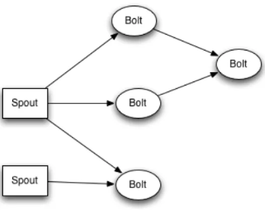
The nodes in the topology are called Components. The components can be either a Spout or a Bolt shown in figure3.1. A spout reads data from an external source and emits it into the topology. Bolts receive data from spout or other bolts. Each bolt is made of a number of tasks, each performing the same operation. The tuple is processed by one of the tasks. The output is emitted back to the topology to be consumed by the next bolt. If the bolt does not have any children, then it is called a Sink. In order to distribute the tuples among the tasks of the bolt, storm supports Stream Groupings. There are eight built-in stream groupings. Storm also provides an interface to define custom groupings.
Figure 3.1: Topology structure indicating Spout and Bolt
of at-most once semantics, Storm guarantees that a tuple is delivered to a component for processing, at most once. If the tuple is lost, say due to machine failure or network latency, Storm does not resend the tuple. These tuples are lost. In case of at-least once semantics, storm makes sure that the tuple is processed at least once. Tuples are replayed when there are failures, and replayed till they are processed. In certain scenarios, it is possible for the same tuple to be processed more than once. Using Trident, a higher level abstraction over Storm’s basic abstractions, exactly-once processing semantics can be achieved. The type of processing semantics used is very much dependent on the type of problem the application is trying to solve.
3.1
Architecture of Apache Storm
A Storm cluster is a collection of machines, also called as Nodes. It consists of two types of nodes, Master Node and Worker Node. At any point of time, there can be only one active master node in the cluster. It can however have as many workers as needed.
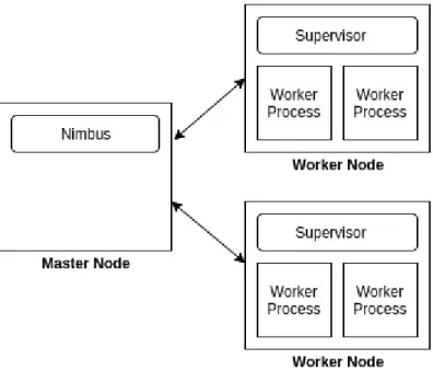
Figure 3.2: High Level Architecture of Apache Storm
Figure3.2provides an overview of the Apache Storm architecture. Master node hosts the Nimbus service. A topology submitted to the cluster for execution is accepted by Nimbus service. It is also responsible for distributing code around the cluster, assigning tasks to the worker nodes and monitoring the nodes for failures.
The scheduling decisions are made by a component called Scheduler. These decisions include allocating the compute resources to the components of the topology during the initialization, scale-out, scale-in operations, and reclaiming the resources after the topology is killed.
Storm provides 4 built-in schedulers, namely Even Scheduler, Isolation Scheduler, Resource Aware Scheduler33and Default Scheduler. The Even scheduler distributes the
among the worker nodes, so that none of the worker nodes sits idle. The Default
Scheduler uses the same strategy of distributing resources evenly. It in fact calls the Even Scheduler internally. The Isolation scheduler lets the user specify which topologies should be “isolated", meaning that they run on a dedicated set of machines within the cluster. Any other topologies executed on those machines will be evicted, before the isolated topologies are scheduled on them. Resource Aware Scheduling allows the user to specify the resources required for the topology. The user can specify the amount of cpu and memory required for each of the component in the topology. If the scheduler is not able to allocate the requested amount of resources, the topology is not scheduled.
Figure 3.3: Architecture of Worker Process1
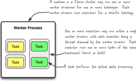
The worker node hosts a daemon called Supervisor. The Supervisor is responsible for receiving assignments from Nimbus and execute it on the worker machine.
Additionally, it communicates the heartbeat status to the Nimbus. The Node may host one more worker process. Each worker process is a JVM process. The worker process may in turn contain one or more Executors. Each Executor is a thread in the worker process, and executes tasks from the same component. The executors may in turn execute one or more tasks. Since each Executor is a single thread, the tasks within the executors are run serially.
The initial number of workers, executors and tasks to be created for the topology, can be specified in the topology description. These initial numbers are called
“parallelism_hint". It basically indicates how many of the tasks are being executed in parallel. Suppose if the component has 8 tasks. If it requests for only one worker and executor, then all the 8 tasks are executed serially on a single thread (Executor). If the component requests two executors, then the tasks are split between two threads, and hence more tasks are executed in parallel.
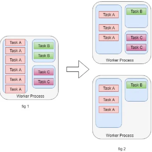
Figure 3.4: Task distribution in a Topology
Figure3.4shows the distribution of tasks in a topology. The user scales out the topology by adding more resources. Even scheduler distributes the tasks evenly across the resources. The 6 tasks of A share a single executor as shown in in the3.4. When the
number of executors are increased to 2, the tasks of A are distributed evenly among the two executors with 3 tasks each. If the number of executor is increased to 3, each executor will execute 2 tasks of A. No changes are seen for Task C, as the number of executors remain same. The same principle holds true when the number of worker processes is increased. The executors are redistributed so that each of the worker process hosts equal number of executors (except in the case when the number of executors is odd).
These numbers can be adjusted during runtime. The name of the command used to adjust the parallelism hint is called “rebalance”. It allows the user to modify the number of workers and executors assigned to a component. Note that the number of tasks in a component cannot be modified by the rebalance command.
Storm version 1.0 and above implement automatic Backpressure. This feature essentially slows down or throttles the process of a parent component whenever a component is congested in the topology. In Storm 1.x the feature can be disabled by configuration options. In Storm 2.0, the feature is redesigned and it is no longer possible to disable it using configuration options. The new implementation uses the state of the internal message buffers to determine if the worker is saturated with messages. If it is, then it sends a backpressure signal to the worker process of parent component
requesting it to stop sending tuples until further notice.
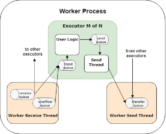
Figure3.5shows the internal message buffers1used in a worker process. The
internal message buffers play a major role in the operation of Storm. The tuples are transferred between workers in batches, essentially making the input pattern bursty. The message buffers essentially insulates the rest of the components from the input pattern. The message buffers are essentially implemented as queues. The worker process uses three queues. The worker receive thread adds the incoming tuples to the Worker Receive queue. If the receive queue is full, the receive thread redirects the incoming tuples to a different queue called Overflow queue. This queue is used by the Backpressure mechanism to send backpressue signal to the parent component. The third queue is the
Figure 3.5: Internal message buffer of worker process
Transfer queue, which acts as a common output buffer for a worker. The tuples emitted by the executors are added to the output queue. The transfer thread then sorts the tuples by destination, collects tuples into batches, and sends them to the destination. Each executor maintains two queues, the Executor Input queue and the Executor Send queue. The tuples from the input queue are sorted and added to the respective executor’s input queue. After operating on the tuple, executor sends the emitted output tuple to the send queue. A send thread then collects the tuples from send queue of executor and adds it to the Output queue of worker.
Storm version 2.0 implements support for cgroup Enforcement. This feature is critical to support Storm in a SaaS flavor and essentially provides the same features as a container. cgroups34(abbreviated from control groups) is a Linux kernel feature that
limits, accounts for, and isolates the resource usage (CPU, memory, disk I/O, network, etc.) of a collection of processes. cgroups allows the provider to enforce resource limits
on the worker process. This can ensure that each worker processes executes in isolation and is not affected by other workers.
We define Input rate for a component as the number of tuples arriving to the component in unit time. The Output rate similarly is the number of tuples emitted by component in unit time. Processing rate is defined as the number of tuples processed by the executors of the component in unit time.
Apache Storm 1.2 introduced a new metric system, to allow users to collect and report the internal state of the cluster. The metric system is based on Dropwizard Metrics. The new system defines a set of API’s that can collect different kind of information. A Timer metric aggregates timing duration and provides duration statistics. A Meter metric measures events and provides an exponentially weighted moving average for one-, five- and fifteen-minutes. A Counter metric simply counts the number of events. In our implementation we extensively use the Meter metric.
Our approach will be using the cgroups feature implemented in Apache 2.0 to create worker process under cgroups, and the metric system to measure the number of tuples moving through each of the internal queues. More details are provided in the
Chapter 4
Stela
Stela is a scale-out algorithm designed to increase the throughput of the topology. Stela achieves this by allocating resources to congested components. The idea is that the increased processing power due to newly allocated resources increases the output from the congested component. This output then propagates downstream and leads to overall increase in throughput.
Stela follows the serial allocation approach. When multiple resources are made available to allocate, Stela decides on each resource in isolation. Once the decision is made, it is not reconsidered or reverted when deciding the allocation for the subsequent resources.
The Stela algorithm for allocating a single resource can be summarized into three tasks as listed below.
1. Identify congested components
2. Measure desirability of each congested component 3. Select a congested component and allocate a resource
If the user provides more than one resource, the above tasks are repeated in order for each resource.
4.1
Identify Congested Components
A component is determined to be congested by the Stela algorithm if the processing rate of the component is less than or equal to its input rate. Essentially, the number of tuples input to the component in a unit time is greater than the number of tuples that can be processed by the same component. An excess of input leads to tuples being dropped. The processing power of the component is proportional to the amount of resources allocated. The algorithm measures the input, output and processing rates of each component in real time at regular intervals. If the input rate for the component is greater than the processing rate, the component is classified as congested. All the congested components of the topology are stored in a list called “congestedMap”
4.2
Measure Desirability of Congested Component
Once the list of congested components are identified, these components or the allocations derived for these components need to be ranked.In order to measure the desirability of each component, the algorithm uses a novel metric called “Expected Throughput Percentage” or ETP. ETP essentially gauges the importance of each node to the overall throughput of the topology. More specifically, the percentage of the total throughput contributed by the subtree of the congested node. To measure the output from a subtree, ETP considers only those sinks that do not contain a congested component in the path as shown in Algorithm1
The ETP for a component is calculated as below. ETP for each congested component is calculated and stored in a map called “ETPMap".
ET P(M) = T hroughputEf f ectiveReachableSinks
Algorithm 1ETP Calculation Algorithm
1: procedureFindETP(Topology topology, Component component)
2: if component.hasChild == falsethen
3: return component.outputRate/throughput(topology)
4: end if
5: subtreeSum = 0
6: queue.add(component.children)
7: whilequeue.isEmpty() == falsedo
8: Component child = queue.pop() 9: if child.isCongested == truethen 10: continue
11: end if
12: if child.hasChild == truethen 13: queue.add(child.children) 14: else 15: subtreeSum += child.outputRate 16: end if 17: end while 18: return subtreeSum/throughput(topology) 19: end procedure
4.3
Choosing The Component
Stela employs a greedy approach to choose among the congested components. It uses the prepared ETPMap to pick the component with the highest ETP. Once the resource is allocated to the component, the input and output for the component and the
downstream components are updated. If k resources are allocated to component M, the new processing rate for the component after allocating one additional resource is calculated as
k+ 1
k ∗CurrentP rocessingRate(M)
Algorithm 2Stela Scaleout Algorithm
1: procedureStela(Topology topology, int numRes)
2: Map<Component, int>allocationMap = null
3: whilenumRes>0do
4: List<Component>congestedMap =
5: getCongestedComponents(topology); 6: forComponent comp : congestedMapdo 7: etp = FindEtp (topology, comp) 8: ETPMap.add(comp, etp)
9: end for
10: Component target = ETPMap.getMaxEtp() 11: currentAlloc = allocationMap.get(target) 12: allocationMap.add (target, currentAlloc+1)
13: numRes = numRes-1
14: update input, output and processing rate of all components
15: end while
16: end procedure
4.4
Drawbacks of Stela
In its outlook, the algorithm is fairly optimistic. The algorithm does not consider the after effects of allocation. Consider fig 1 for example.
If the ETP of B is greater than C, the resource is allocated to component B. However, the increase in the throughput is not realized as D gets congested. Stela does not check if the downstream components are able to handle the additional output from component B. Stela does not examine or measure the consequences of an allocation before making the allocation. So it is unable to detect scenario mentioned above. As a result, Stela produces less than optimal allocations in the following two cases. First, downstream nodes do not have the capacity to handle the increased output. Second, the degree of congestion of a component is not taken into account. That is, a lightly congested
component is treated the same as a heavily congested component. It is possible that the increase in the output on a lightly congested component might be too little to improve the throughput significantly. Thus being able to predict the after effects, and estimate the increase in throughput could help overcome these limitations, which motivates our
Chapter 5
Scale-Out Algorithm
5.1
Goals and Assumptions
We recognize scaling to be an important operation in the cloud, and is critical to the success of such a service. Our work proposes an algorithm to a support scale-out operation. More specifically, given a set of resources for scheduling our algorithm provides an allocation to decongest components and maximize the throughput increase. Additionally it attempts to predict the state of the topology if the suggested allocation is indeed committed.
The scale out algorithm focuses on maximizing the throughput of the topology by allocating resources to congested components.
In order to narrow the scope and simplify the problem, our work makes the following assumptions about the topology and the cluster.
• The resources are made available in the form of resource units. Each resource unit provides a fixed amount of processing power, that is the cpu power on a machine of a cluster. The processing power provided by each resource unit is equal. This can be enforced by using cgroups or containers.
to components. It is assumed that network capacity is infinite, and the effects of network latency can be ignored.
• We assume that when a topology reaches a steady state, the input, processing and output rates of the components remain nearly constant.
• It is assumed that the cluster is configured to disable backpressure enforcement. When backpressure is enforced, Storm throttles the input whenever a component gets congested. Thus a single component can become the bottleneck for the entire topology. This not only limits user’s ability to control execution, but can also adversely affect resource usage. It prohibits components from fully utilizing the resources allocated to it, as the input can get throttled due to congestion in a different part of the topology.
The flip side of the argument is that the tuples can get dropped when backpressure is disabled. Our algorithm caters to the same class of topologies as Stela, where loss of tuples is tolerable. In the future work section, we propose an approach to further improve backpressure system, where the loss of tuples can be avoided.
The above assumptions are consistent with those made by Stela. In our approach, each component is free to scale as required. In a cloud environment this allows for maximum flexibility and control over how the resources are allocated and used by the topology. The user can prioritize certain components over others, sometimes at the expense of congesting components of lower priority.
5.2
Approach and Design
The general approach taken by our algorithm is very much contrary to Stela. Our algorithm chooses to use Batch allocation and measures the effects of an allocation before it is made. Our algorithm is conservative and considers allocations that do not
worsen or introduce any new congestion in the downstream components. We propose a simple model to predict the input and output rates of the components after an allocation is made. Finally, we recognize the limitations of our algorithm and provide an approach to incorporate Stela as a co-scheduler. Combining both algorithms provides better allocations to a larger set of scenarios than each of the individual algorithms.
5.2.1
Resource Units
The resources are provisioned in terms of resource units. Each resource unit is guaranteed a certain processing power by using cgroups. All the resource units have equal processing power allocated to them. The user can request resource units to be allocated to a component. The component uses these resources provided to execute its tasks. For the rest of the discussion the term resource is used to indicate resource unit.
5.2.2
Batch Allocation
Batch allocation strategy is favored by our algorithm. Serial allocation strategy does not take the the number of resources provided into consideration before making scheduling decisions. When a resource is allocated to a component, the output propagates through its subtree. If any of the components in the subtree are congested, then additional resources need to be allocated. Knowledge of the number of resources needed by a subtree to achieve required throughput and the number of resources provided to a user could be helpful in deciding allocations.
5.2.3
Compute Model
In order to estimate the state of the components in the topology we build a simple model. The model serves the following purposes
2. Allows the algorithm to predict if the allocation causes a congestion in the subtree 3. Allows the algorithm to estimate the throughput for an allocation
The processing power for components are supplied in resource units. So logically, we can view components as made of resource units. Components are profiled to measure the maximum input, output and processing rates when executed in a single resource unit. The total rates for a component is obtained by multiplying the number of resources allocated to the component with their profiled rates. The components are organized in a structure similar to the topology complying to their parent-child relationships. The network capacity is assumed to be unlimited. We define the following properties for the component.
unitCountis the total number of resource units allocated to a component.
congestionis a flag set to a component to indicate if it is congested. A component is
determined to be congested if the inputRate exceeds processingRate.
inputRateis the total number of tuples flowing into a component in unit time. It
can be calculated as the aggregate of the inputs coming into all the resource units that are executing the tasks of the given component M. Note that this accounts for both processed tuples and dropped tuples.
inputRate(M) = ΣinputRate(resource units),∀resource unit∈M
droppedRateis the number of tuples dropped by the component if the processing
power is not sufficient. This is measured from the component.
droppedRate(M) = inputRate(M)−processingRate(M)
could be less than or equal to the inputRate.
inputRate(M) = processingRate(M) +droppedRate(M)
outputRateis the total number of tuples flowing out of a component in unit time.
This is calculated as the aggregate output of all the resource units that are executing the tasks of the given component.
outputRate(M) =processingRate(M)∗outInRatio(M)
outInRatiois a simple ratio of the output to processing rate of a component.
outInRatio(M) = outputRate(M)
processingRate(M)
maxProcessingRateis the maximum input the component can process. This is
determined by the amount of resources allocated to component. Max input for a component is profiled for a resource unit beforehand. Given ‘n’ is the number of resources allocated to component M,
maxP rocessingRate(M) =maxP rocessingRate(resourceunit)∗n
childOutputRatio(i)is the ratio of tuples destined for theithchild component of
component M. This is profiled beforehand.
childOutputRatio(i) = rateof tuples assigned to childi
outputRate(M)
throughputof a topology is calculated as the sum of all the totalOutput of leaf nodes.
throughputResourceRatiois calculated as the ratio of increase in throughput to the
number of resources allocated. Given ‘n’ is the number of resources allocated to a subtree rooted at M,
throughputResourceRatio(M) = increaseInT hroughput
n
5.2.4
Calculating Throughput for Allocation
The current throughput can be directly obtained by measuring the output of leaf
components. This section describes an approach to calculate the throughput when a new resource is allocated.
As per the assumptions made, the processing rate is entirely dependent on the cpu allocated. If ‘n’ is the current number of resources allocated to a component M. When a new resources is added, the maximum processing rate and thus the maximum output rate of the component changes.
• The new processing rate is calculated as shown below.
newM axP rocessingRate(M) = (n+ 1)
n ∗maxP rocessingRate(M)
• The new output rate is accordingly calculated as below.
newOutputRate(M) = newP rocessingRate(M)∗outInRatio(M)
The children use the same procedure to update their processing, input and output rates. These changes are propagated further till all the components in the subtree are updated. We update the values for each component in the subtree by using a modified BFS traversal. The new throughput of the topology is then calculated as the sum of the output of all the leaf components with its updated output rates. It is to be noted that the
model is simple and makes assumptions about the topology. In our testing we show that the model predicts the rates of the components with reasonable accuracy.
5.2.5
Strategy
This section describes the high level strategy used by our algorithm. The user provides the topology and the number of resources to be allocated. The algorithm works on the principle that the throughput of the topology is constrained due to congestions in components and the output rate can be increased by decongesting components.
An allocation is defined as a map of components associated with the number of additional resources to be allocated. The allocation map is initialized to a list of all the components mapped to the value 0 indicating no additional resources are currently allocated to any component. When the algorithm decides to allocate a resource to the component, the value corresponding to the component in the map is incremented.
Similar to Stela, the algorithm starts by identifying all the congested components in the topology. Components are profiled for their maxProcessingRate. A component is determined to be congested if the maxProcessingRate for the component is less than the inputRate. This can also be determined by measuring the droppedRate. If a component has a droppedRate above a threshold, then the component is congested. In our work we use the maxProcessingRate.
The strategy is to allocate resources to a congested component to increase its output. If any of the components in the subtree gets congested additional resources can be allocated till it is no longer congested. It is important to note that we do always decongest a root component completely every time it is considered. The extent to which the root component is decongested depends on the output the subtree can support with the remaining resources. Thus the resources allocated can be split into two parts, the ones allocated to congested root component, and the ones allocated to subtree to sustain the output. If the total number of resources required is more than the resources available
then this introduces or worsens congestion of at least one component in the subtree. For each congested component, the algorithm allocates resources to the root congested component incrementally. For each iteration one additional resource is allocated until the root component is completely decongested. After each allocation to the root component, the algorithm propagates the increased output through its subtree. If any of the components in the subtree gets congested, the number of additional
resources is calculated for the component. The new output is then propagated through its child components. At the end of the subtree, the algorithm obtains the total number of additional resources needed by the subtree, as well as the throughput increase caused by the additional resources. If the total number of resources exceeds the number of resources provided, then the allocation is rejected.
Each valid allocation is stored in a map keyed by the root component and the number of resources allocated to the root. The map also stores some useful information like the throughput increase, number of resources needed and the
throughputResourceRatio. The list of valid AllocationMap are maintained in a list called AllocationMapList.
The AllocationMapList is sorted in decreasing order of throughputResourceRatio. The algorithm tries to select as many allocations as possible in order, as long as the total number of resources required for the allocations is less than or equal to the resources provided by the user. These allocations are combined together to obtain optimal allocation. Though we are selecting allocations in a greedy serial order, the number of resources allocated at each step may be greater than 1. So essentially we are allocating resources in batches. A further improvement to this method is to use an algorithm similar to the one that solves knapsack problem to ensure the selection of allocations is optimal as well.
Next, we describe how to combine allocations. Though each of the allocations are calculated separately, it is possible that some of the components in these allocation
overlap with each other. Consider two allocations A and B. If the root of allocation B is a descendent of the root of allocation A then allocation A is a superset of B. This follows from the rule that the algorithm considers only the allocations that completely decongest all of the descendents of a subtree rooted at a congested node. Since allocation A is a superset of B, if A is chosen then B is discarded from our solution.
5.2.6
Residual Resources
Our algorithm uses a greedy approach similar to Stela to select allocations from the AllocationMapList. This number of resources allocated in each greedy selection is dictated by the allocation considered in the allocationMap. It is possible that in some cases not all the provided resources can be allocated. There are cases where the remaining resources are not sufficient to satisfy any allocation from the
AllocationMapList. When this happens, these resources are called Residual resources. Many approaches can be taken to allocate the residual resources. One approach would be to choose an unused allocation from the sorted allocationMapList with the highest throughputResourceRatio and allocate resources to components encountered in a Deapth First Search (DFS) or Breadth First Search (BFS) traversal. Since the number of resources are not sufficient the subtree becomes partially congested. The outcome of this approach can vary greatly depending on the number of remaining resources, the selected allocation and the topology itself.
We select an unused allocation with the lowest number of resources required instead of one with the highest throughputResourceRatio. The idea is that even if we worsen the state of congestion with the residual resources, fewer resources would be needed to decongest these newly created congestions. Resources could be allocated to decongest these components the next time user wants to scale out the topoplogy.
Once the allocation is selected, we allocate one residual resources to the root component. The increased output now causes new components in the subtree to
congest. Thus we have a problem of allocating the remaining residual resources to the subtree to decongest it. This is exactly the same problem as the scale out problem, except for in this case we are trying to scale out a subtree instead of the entire topology. This gives us a good premise to use recursion to solve the problem.
A new topology is created which mirrors the subtree. One resource is allocated to the root of the subtree and our algorithm could then be called with the remaining number of residual resources to obtain an optimal allocation for the subtree of newly congested nodes. If all of the resources are still not allocated to the subtree because they are not sufficient to decongest any node and its descendents, the allocation with the lowest resource requirement for the subtree can again be selected and a new topology can be created. This process can be repeated until all the resources are allocated. A residual allocation map is created by combining the optimal allocation obtained from each of the steps to the optimal allocation for the main topology. The algorithm section provides more details about this process.
Thus the output from our algorithm to the user would be two allocation maps • optimalAllocationMap - does not worsen the congestion in the topology. This does
not contain allocations for residual resources
• residualAllocationMap - is the combined map obtained by merging the
optimalAllocationMap with the residual map obtained by the aforementioned recursive algorithm.
5.2.7
Algorithm
The algorithm expands upon the strategy outlined in the previous section. We first introduce the two main data structures used in the algorithm as shown in Algorithm
5.2.7. Allocation is a simple map structure, that maps a component to the number or resources allocated to it. Each component is initialized to 0 resources and can be
incremented or decremented as needed. The second structure AllocationMap is used to associate an allocation with a congested component. For each congested component in the topology, the algorithm tries to decongest it and its subtree by allocating resources. The root of the subtree is stored in headComp. Our algorithm explores options to
partially decongest the root node, so headRes stores the number of resources allocated to just the root component of a subtree.
Algorithm 3Data Structures
Allocation{comp1 :nRes1, comp2 :nRes2, ...};
. foreach componentcompiin the topology,nResiis number of resources allocated to
ith component.
AllocationMap{
headComp,
headRes, .resources allocated to headComp of a subtree
Allocation, .for the subtree
T hroughput, .throughput increase due to the Allocation totRes, .sum ofnResiin the Allocation
throughputResRatio
}
The scale out algorithm as shown in Algorithm4accepts the topology and number of resources to be allocated from the user. The topology contains the runtime
information like the input rate, processing rate, output rate etc of each component. The algorithm can be divided into four parts.
• Get allocation for the topology using the approach described in previous section (line : 2). For the rest of the discussion we refer to it a predictive approach. • Allocate the residual resources to the sub topology (lines 6-14).
• Get allocation using Stela approach (line : 15).
• Pick the allocation that is predicted to give the higher throughput (lines 16-18). Line 2: gets the allocation using our predictive approach as described in Algorithm
congestion of any component stored in optimalAlloc variable. The second is allocaTable. It is essentially the list of all congested components and respective allocations to
decongest their subtree. These will be used to allocate residual resources.
Lines 6-13 allocate any resources not allocated by predictiveAlloc. Line 7 sorts unused AllocationMaps in allocTable, picks the allocation that needs the least number of resources say c. We use our predictiveAlloc algorithm to allocate the residual resources. We creates a new topology by copying the components of subtree under the headComp of allocation c. This new topology is used as input in Line 11. Line 10 allocates a resource to the head node of the new topology. This causes some of the components of the subtree to get congested. Line 11 tries to allocate the remaining resources to the new topology. The optimal allocation returned from the step is used to update residualAlloc. The remaining unallocated resources are updated, and the loop is executed with the new AllocationMapList till all the resources are allocated. Once all the resources are allocated residualAlloc from our algorithm is obtained. Line 14 obtains allocation using stela algorithm. We then pick the allocation with the higher throughput and apply it for the user.
The merge operation in line 12 is performed by adding the resources allocated to each component in both allocation maps. For example if map 1 allocates 1 resource to component A 2 resources to component B, and map 2 allocates 0 resources to component A and 2 resource to component B, then the merged map allocates 1 resource to
component A and 4 resources to component B.
Algorithm5gives the pseudocode of the predictive strategy we discussed in the previous section and can be summarized into th following steps. Line 2 gets a list of congested components in the topology. Lines 5-25 obtain a list of candidate allocations. Essentially for each component in congested list, one or more resources are allocated to head component. By doing a bfs traversal through its subtree the number of resources needed to decongest the whole subtree is calculated as shown in Lines 12-16. If the total
Algorithm 4Scale out Algorithm
1: procedureScaleOut(Topology topology, int numRes)
2: {optAlloc, allocTable} =
3: PredictiveAlloc (topology, numRes); 4: Allocation residualAlloc = optimalAlloc 5: excessRes = numRes - countRes(optAlloc) 6: while