ESTIMATING AND FORECASTING GARCH
VOLATILITY IN THE PRESENCE OF OUTLIERS*
M. Ángeles Carnero, Daniel Peña and Esther Ruiz**
WP-AD 2008-13
Corresponding author: M.A. Carnero. Dpt. Fundamentos del Análisis Económico, Universidad de Alicante. Campus de S. Vicente del Raspeig, 03690, Alicante, Spain. Tel: +34 965903400 (ext. 3255), Fax: +34 965903898. E-mail: [email protected].
Editor: Instituto Valenciano de Investigaciones Económicas, S.A. Primera Edición Octubre 2008
Depósito Legal: V-4540-2008
IVIE working papers offer in advance the results of economic research under way in order to encourage a discussion process before sending them to scientific journals for their final publication.
* Financial support from project SEJ2005-02829/ECON by the Spanish Government is gratefully acknowledged. Thanks to the participants at the ESEM07 meeting in Budapest and Simposio de Análisis Económico in Granada and at seminars at Universidad de Alicante, Universidad Complutense de Madrid and Universidad Carlos III de Madrid for helpful comments and suggestions. We are also very grateful to the comments of one anonymous referee that have improved this paper. Any remaining errors are our own.
ESTIMATING AND FORECASTING GARCH VOLATILITY IN THE PRESENCE OF OUTLIERS
M. Ángeles Carnero, Daniel Peña and Esther Ruiz
ABSTRACT
The main goal when fitting GARCH models to conditionally heteroscedastic time series is to estimate the underlying volatilities. It is well known that outliers affect the estimation of the GARCH parameters. However, little is known about their effects when estimating volatilities. In this paper, we show that when estimating the volatility by using Maximum Likelihood estimates of the parameters, the biases incurred can be very large even if estimated parameters have small biases. Consequently, we propose to use robust procedures. In particular, a simple robust estimator of the parameters is proposed and shown that its properties are comparable with other more complicated ones available in the literature. The properties of the estimated and predicted volatilities obtained by using robust filters based on robust parameter estimates are analyzed. All the results are illustrated using daily S&P500 and IBEX35 returns.
JEL classification: C22
1
Introduction
It is usual to observe that long time series of financial returns have observations that can be considered as outliers. On the other hand, it is widely accepted that financial returns are conditionally heteroscedastic. Distinguishing outliers from conditional het-eroscedasticity is not an easy task since both phenomena may generate excess kurtosis and autocorrelations of squares; see, for example, Carnero et al. (2007). However, their implications are different since conditional heteroscedasticity implies the possibility of forecasting future volatilities while outliers are unpredictable.
Previous research on the topic has focused on the effects of outliers on the Maximum Likelihood (ML) estimator of the GARCH parameters assuming a normal distribution for the innovations; see, for example, Sakata and White (1998), van Dijk et al. (1999), Muler and Yohai (2007) and Carnero et al. (2007). Nevertheless, the main interest of practitioners in this area is not to estimate the parameters but to estimate the underlying conditional variance which is considered as a useful measure of uncertainty. Such a measure is of central importance in many financial models like, for example, option valuation or risk management models. It is also important to have accurate estimations of the volatility when computing risk using, for example, the Value at Risk (VaR) or the Expected Shortfall based on predictive densities of returns. Furthermore, the estimation of the volatility is crucial for the efficient estimation of the conditional mean dependency and the construction of prediction intervals.
In this paper we investigate the effects of outliers on the estimation of the underlying volatility. We show that the volatilities estimated by using the GARCH specification with ML estimates of the parameters can be positively biased, not only in the period of time when the outlier occurs, but also through all the sample period. We also show that their biases are not a linear function of the biases of the estimators. They can be very important even when the biases in the estimated parameters are very small. Due to this non linearity, it is possible to observe series where parameter estimates close to the true values lead to volatility estimates with larger biases than others computed with worse estimates of the parameters. We will see that the marginal variance plays an important role in the estimation of the volatility. Outliers affect in a serious way the marginal variance, consequently, it is important to take into account the potential presence of these atypical observations. There are two alternative strategies to deal with outliers. The first one is to identify and correct outliers before estimating the parameters of the equation governing the evolution of the conditional variance. The second one is to use robust methods to estimate both the parameters and the underlying volatilities.
Detecting and filtering outliers would generate volatility estimates with smallest Mean Square Error (MSE) when the true outliers are detected as such but the avail-able methods to detect outliers are very costly computationally. For example, the procedure proposed by Hotta and Tsay (1998) is based on adding an additional
pa-rameter at a time to represent the outlier effect and testing for its significance using a Lagrange Multiplier (LM) test. If the parameter is found significant, the corresponding observation is identified as an outlier. However, the distribution of the LM statistic has to be simulated each time an outlier is found. Alternatively, Doornik and Ooms (2004) propose a test that uses the largest standardized residual as the outlier candidate and performs a Likelihood Ratio test with respect to a model with dummy variables in both the level and the volatility equations. As a result, this test provides an estimate of the location and size of the outlier. This procedure is computationally simpler than the one proposed by Hotta and Tsay (1998) given that its asymptotic distribution can be approximated from an extreme value distribution that does not require simu-lation. However, it is an iterative procedure that works on single deletion diagnostics and it is not designed to deal with patches of outliers. More recently, Grossi (2004) has proposed a forward search to look for outliers in GARCH models. The forward search overcomes the drawbacks of single deletion methods because it monitors outlier diagnostics starting from an initial subset free from outliers.
In this paper we propose to estimate the underlying volatilities using robust proce-dures. The estimation is done in two steps. First, a robust estimator is implemented to estimate the parameters of the GARCH model. Second, a robust filter can be used to estimate the underlying volatilities. We consider three alternative estimators for the robust estimation of the GARCH parameters. The first one is a Quasi Maximum Likelihood (QML) estimator based on maximizing the Student-t log-likelihood where
the degrees of freedom, ν, are considered as an unknown parameter. This estimator,
denoted by QML-t, was proposed by Bollerslev (1987) and it is robust when estimating the ARCH parameter but it looses part of its robustness when estimating the persis-tence parameter of the GARCH(1,1) model; see Carnero et al. (2007). Consequently, we propose a second estimator based on modifying the QML-t estimator by changing the specification of the conditional variance to bound the propagation of the outlier effect. We call this modified estimator Bounded QML-t (BQML-t). The third robust estimator is the Bounded-M (BM) estimator proposed by Muler and Yohai (2007). We show that the BQML-t estimator is simpler than the BM estimator while having com-parable efficiency and robustness properties when the number and size of the outliers are not very large. We compare the performance of the alternative estimators in the presence of additive level outliers, as it is usual in this literature, but also when the outliers are volatility outliers.
Once the GARCH parameters have been estimated by one of the robust estimators previously mentioned, the underlying volatilities can be estimated by a robust filter. Muler and Yohai (2007) propose a filter based on trimming all the standardized ob-servations larger than a given threshold by equalling them to the threshold. In this paper, we also consider an alternative filter in which the observations larger than the threshold are set equal to their conditional standard deviations. We analyze the finite
sample properties of the robust filters and show that the volatility estimates based on them reduce the positive biases and the MSE observed in the ML estimates. Obviously, the estimation of the underlying volatilities affects the construction of prediction in-tervals for future values of the series of interest. Therefore, we also analyze the effects of outliers on the construction of prediction intervals for future values of GARCH(1,1) series. As expected, in the presence of outliers, the prediction intervals based on ML estimates have coverage larger than the nominal.
The rest of the paper is organized as follows. Section 2 analyzes the effects of outliers on the ML estimation of the underlying volatility. Section 3 proposes a robust estimator of the parameters and compares its finite sample properties with those of the ML and BM estimators. Section 4 studies the properties of the robust estimates of the underlying conditional variances and compare them with those of the estimates based on ML. Section 5 contains an empirical application where the underlying volatilities of daily S&P500 and IBEX35 returns are estimated and predicted. Finally, section 6 concludes the paper.
2
Effects of outliers on the estimation of the
under-lying volatility
In this section, we analyze the effects of outliers on the underlying volatilities when they are estimated by substituting the parameters in the GARCH equation by their ML estimates.
To simplify the problem, consider that the series y∗
t has been generated by an
uncorrelated GARCH(1,1) model. In this case, there is no distinction between additive
and innovative outliers. Therefore, a series contaminated by k consecutive outliers of
size ω at times τ,...,τ +k−1, is given by
yt=yt∗+sign(yt∗)ωIt (1)
with
y∗
t =εtσt
whereεt is a Gaussian white noise process andIt is a dummy variable being one when
t=τ, ..., τ+k−1 and zero otherwise. The specification of the volatility,σ2
t,depends on
the type of the outlier. Following Hotta and Tsay (1998), outliers in GARCH models can be classified as level (LO) or volatility (VO) outliers. A LO does not affect the conditional variance which is given by
σt2 =α0+α1yt∗−21+βσt2−1 (2)
whereas if a VO is present, the conditional variance is given by
In both cases, we assume that the parameters satisfy the positivity and stationarity
restrictions, i.e. α0 >0, α1 ≥0, β≥0 and α1+β <1.
Denote by nαbM L
0 ,αbM L1 ,βbM L
o
the ML estimator of the GARCH (1,1) parameters. If the parameters are estimated as usual by ML, the estimated volatilities (denoted
from now on by bσtM L
2
) are given by
b
σtM L2 =αbM L0 +αbM L1 yt2−1+βbM L σbtM L−12. (4)
Consider now that there is an isolated VO at timet =τ. The error in the estimation
of the underlying volatility at time t, denoted by ξV O
t , is the difference between the
estimated and true volatilities in (4) and (3) respectively, and it is given by ξtV O = bσtM L2−σt2 = (αbM L0 −α0)+(αb1M L−α1)yt2−1+(βbM L−β)σ2t−1+βbM L
b
σtM L−12−σt2−1 (5) In expression (5) it is possible to observe that the expected error in the estimation of the underlying volatility depends on the biases of the estimator of the parameters. However, the expectation of the last term in (5) depends also on the covariances be-tween the estimators and on expections of non-linear functions of the estimators. To see this point more clearly, consider the following alternative expression of the error in the estimation of the underlying volatilities,
ξtV O = (αbM L 0 −α0) 1−βbM Lt−1 1−βbM L + (αb M L 1 −α1) t−2 X i=0 b βM Liy2t−1−i+ (βbM L−β) t−2 X i=0 b βM Liσt2−1−i+βbM Lt−1 σb1M L2−σ12. (6)
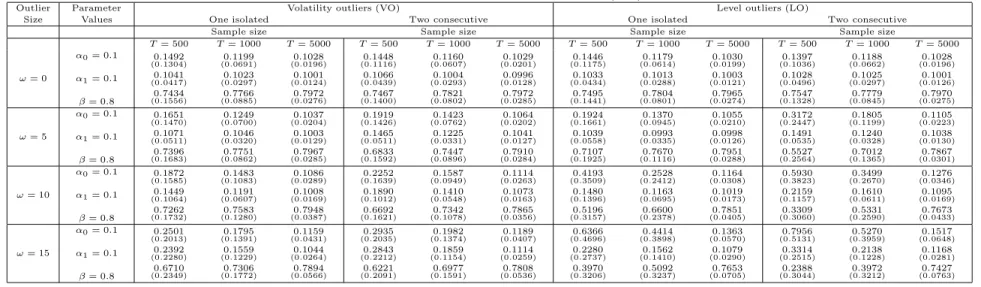
Consequently, to understand the errors in estimating the underlying volatilities, it is of interest to consider first, the biases incurred when estimating the GARCH parameters by ML. Previous research has focused on the analysis of the biases of the ML estimator in the presence of LO. However, little is known about its properties when the series are contaminated by VO. Consequently, we have carried out a small Monte Carlo experiment generating 1000 series by a GARCH(1,1) model with parameters
α0 = 0.1, α1 = 0.1 and β = 0.8. The sample sizes considered are T = 500, 1000 and
5000. The sample sizes and the parameters have been chosen to resemble the values usually encountered when analyzing real data. The series have been contaminated at
time τ = T /2 by first an isolated and second by two consecutive VO. Table 1, that
reports the Monte Carlo means and standard deviations, shows that the effects of VO are similar regardless of whether they are consecutive or isolated. The biases are slightly larger when the outliers are consecutive and the standard deviations are very
similar in both cases. In any case, α0 and α1 are in average, overestimated and β is
underestimated.
However, as we have seen before, the biases when estimating the underlying volatili-ties not only depend on the biases of each of the estimators but also on the expectations of some non-linear functions of the estimators. Therefore, to illustrate this point, we
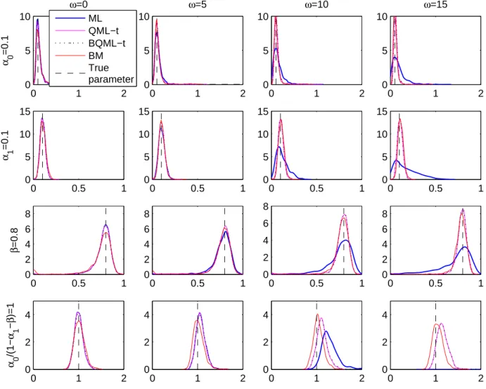
have plotted in Figure 1 kernel densities of the Monte Carlo ML estimates of α0, α1
and β together with the marginal variance given by α0/(1−α1 −β), obtained when
T = 1000 and the series are contaminated by an isolated VO. This figure shows that
the bias when estimating the marginal variance can be very large even in cases when the biases of each of the individual parameters are moderate. Observe that when the
size of the outlier is large, i.e. ω = 15, the density is concentrate so far from the true
value that it does not appear in the figure where only the left tail can be seen. As a con-sequence, the volatilities corresponding to periods of time previous to the appearance of the outlier will be positively biased.
At time t = τ + 1, the error in (6) is positive and larger than before because y2
τ
is large while σ2
τ is not affected by the outlier. Therefore, we expect that, in general,
the volatility is overestimated by a very large amount just after the outlier appears.
Then, at time t > τ + 1, both y2
t and σt2 are large and the errors tend exponentially
towards their previous mean with parameterβbM L. This pattern is similar regardless of
whether the VO are isolated or consecutive. The only difference is that, in the presence of consecutive VO, the biases in the estimated volatilities are larger due to larger biases in the estimated parameters as reported in Table 1.
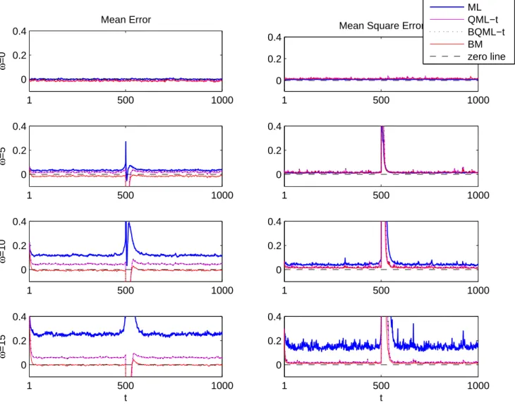
Figure 2 illustrates the biases and MSE found when estimating the underlying
volatility in the presence of an isolated VO at time τ =T /2. The thicker line
corre-sponds to the mean at timet across 1000 replicates of the errors,ξV O
t ,for a sample size
ofT = 1000 and outlier sizes considered before. Note that, if no outliers are present in
the data, the marginal variance of yt is one and the true conditional variances should
oscillate around this value. Therefore, the relative mean errors in the estimation of the volatilities could be rather large when the sample sizes are moderate even if there is just a single outlier. As Figure 2 shows, if a VO of size 15 standard deviations is present
in a GARCH(1,1) series of size T = 1000 and volatility is estimated by ML without
taking into account the presence of that extreme observation, the true volatility would
be overestimated more than 25% at any point of timetand more than 100% in periods
right after the outlier appearance. Notice that, even for smaller outliers, the distortion of the estimated volatilities corresponding to periods of time after the outlier could be very severe and it could take a large number of observations to converge back to the mean. The second column of Figure 2, that plots the Monte Carlo MSE of the estimated volatilities, shows that they can be rather large specially after the period of time when the outlier appears.
The errors, ξV O
Figure 1: Kernel density estimates of estimated parameters of simulated GARCH(1,1)
series of size T = 1000 contaminated with a single VO
0 1 2 0 5 10 ω=0 α 0 =0.1 0 1 2 0 5 10 ω=5 0 1 2 0 5 10 ω=10 0 1 2 0 5 10 ω=15 0 0.5 1 0 5 10 15 α 1 =0.1 0 0.5 1 0 5 10 15 0 0.5 1 0 5 10 15 0 0.5 1 0 5 10 15 0 0.5 1 0 2 4 6 8 β =0.8 0 0.5 1 0 2 4 6 8 0 0.5 1 0 2 4 6 8 0 0.5 1 0 2 4 6 8 0 1 2 0 2 4 α 0 /(1− α 1 − β )=1 0 1 2 0 2 4 0 1 2 0 2 4 0 1 2 0 2 4 ML QML−t BQML−t BM True parameter
Table 1: Mean and Standard deviations of ML estimator of GARCH(1,1) model in the presence of outliers
Outlier Parameter Volatility outliers (VO) Level outliers (LO)
Size Values One isolated Two consecutive One isolated Two consecutive
Sample size Sample size Sample size Sample size
T= 500 T= 1000 T= 5000 T= 500 T= 1000 T= 5000 T= 500 T= 1000 T= 5000 T= 500 T= 1000 T= 5000 ω= 0 α0= 0.1 α1= 0.1 β= 0.8 0.1492 (0.1304) 0.1041 (0.0417) 0.7434 (0.1556) 0.1199 (0.0691) 0.1023 (0.0297) 0.7766 (0.0885) 0.1028 (0.0196) 0.1001 (0.0124) 0.7972 (0.0276) 0.1448 (0.1116) 0.1066 (0.0439) 0.7467 (0.1400) 0.1160 (0.0607) 0.1004 (0.0293) 0.7821 (0.0802) 0.1029 (0.0201) 0.0996 (0.0128) 0.7972 (0.0285) 0.1446 (0.1175) 0.1033 (0.0434) 0.7495 (0.1441) 0.1179 (0.0614) 0.1013 (0.0288) 0.7804 (0.0801) 0.1030 (0.0199) 0.1003 (0.0121) 0.7965 (0.0274) 0.1397 (0.1036) 0.1028 (0.0496) 0.7547 (0.1328) 0.1188 (0.0662) 0.1025 (0.0297) 0.7779 (0.0845) 0.1028 (0.0196) 0.1001 (0.0126) 0.7970 (0.0275) ω= 5 α0= 0.1 α1= 0.1 β= 0.8 0.1651 (0.1470) 0.1071 (0.0511) 0.7396 (0.1683) 0.1249 (0.0700) 0.1046 (0.0320) 0.7751 (0.0862) 0.1037 (0.0204) 0.1003 (0.0129) 0.7967 (0.0285) 0.1919 (0.1426) 0.1465 (0.0511) 0.6833 (0.1592) 0.1423 (0.0762) 0.1225 (0.0331) 0.7447 (0.0896) 0.1064 (0.0202) 0.1041 (0.0127) 0.7910 (0.0284) 0.1924 (0.1661) 0.1039 (0.0558) 0.7107 (0.1925) 0.1370 (0.0945) 0.0993 (0.0335) 0.7670 (0.1116) 0.1055 (0.0210) 0.0998 (0.0126) 0.7951 (0.0288) 0.3172 (0.2447) 0.1491 (0.0535) 0.5527 (0.2564) 0.1805 (0.1199) 0.1240 (0.0328) 0.7012 (0.1365) 0.1105 (0.0223) 0.1038 (0.0130) 0.7867 (0.0301) ω= 10 α0= 0.1 α1= 0.1 β= 0.8 0.1872 (0.1585) 0.1449 (0.1064) 0.7262 (0.1732) 0.1483 (0.1083) 0.1191 (0.0607) 0.7583 (0.1280) 0.1086 (0.0289) 0.1008 (0.0169) 0.7948 (0.0387) 0.2252 (0.1639) 0.1890 (0.1012) 0.6692 (0.1621) 0.1587 (0.0949) 0.1410 (0.0548) 0.7342 (0.1078) 0.1114 (0.0263) 0.1073 (0.0163) 0.7865 (0.0356) 0.4193 (0.3509) 0.1480 (0.1396) 0.5196 (0.3157) 0.2528 (0.2412) 0.1163 (0.0695) 0.6600 (0.2378) 0.1164 (0.0308) 0.1019 (0.0173) 0.7851 (0.0405) 0.5930 (0.3823) 0.2159 (0.1157) 0.3309 (0.3060) 0.3499 (0.2670) 0.1610 (0.0611) 0.5331 (0.2590) 0.1276 (0.0346) 0.1095 (0.0169) 0.7673 (0.0433) ω= 15 α0= 0.1 α1= 0.1 β= 0.8 0.2501 (0.2013) 0.2392 (0.2280) 0.6710 (0.2349) 0.1795 (0.1391) 0.1559 (0.1229) 0.7306 (0.1772) 0.1159 (0.0431) 0.1044 (0.0264) 0.7894 (0.0566) 0.2935 (0.2035) 0.2843 (0.2212) 0.6221 (0.2091) 0.1982 (0.1374) 0.1859 (0.1154) 0.6977 (0.1591) 0.1189 (0.0407) 0.1114 (0.0259) 0.7808 (0.0536) 0.6366 (0.4696) 0.2280 (0.2737) 0.3970 (0.3206) 0.4414 (0.3898) 0.1562 (0.1410) 0.5092 (0.3237) 0.1363 (0.0570) 0.1079 (0.0290) 0.7653 (0.0705) 0.7956 (0.5131) 0.3314 (0.2515) 0.2388 (0.3044) 0.5270 (0.3959) 0.2138 (0.1228) 0.3972 (0.3212) 0.1517 (0.0648) 0.1168 (0.0281) 0.7427 (0.0763) 24
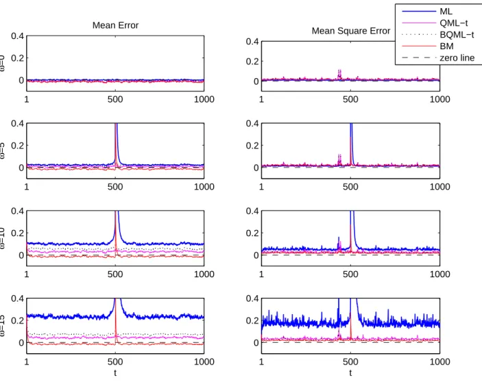
Figure 2: Monte Carlo means and MSE of ξV O
t in the presence of one isolated VO
computed with different estimators and filters in GARCH(1,1) series of size T = 1000
1 500 1000 0 0.2 0.4 Mean Error ω =0 1 500 1000 0 0.2 0.4
Mean Square Error
1 500 1000 0 0.2 0.4 ω =5 1 500 1000 0 0.2 0.4 1 500 1000 0 0.2 0.4 ω =10 1 500 1000 0 0.2 0.4 1 500 1000 0 0.2 0.4 ω =15 t 1 500 1000 0 0.2 0.4 t ML QML−t BQML−t BM zero line
Table 2: Estimation results for daily returns series
S&P 500 IBEX 35 α0 α1 β η α0 α1 β η ML 0.0141 (0.001) 0(0.0856.002) 0(0.9047.004) - 0(0.0278.004) 0(0.1073.010) 0(0.8792.009) -QML-t 0.0058 (0.002) 0(0.0540.008) 0(0.9416.008) 0(0.1588.003) 0(0.0157.005) 0(0.0919.014) 0(0.9023.015) 0(0.1051.002) BQML-t 0.0058 (0.002) 0(0.0540.008) 0(0.9416.008) 0(0.1588.003) 0(0.0157.005) 0(0.0919.014) 0(0.9023.015) 0(0.1051.002) BM 0.0051 0.0559 0.9345 - 0.0088 0.0853 0.9060
-larger compared to those when there is just one single VO, due to the small differences in the estimated parameters, as shown in Table 1. Therefore, the plots of the mean errors and their corresponding MSE, obtained in this case, are very similar to the ones represented in Figure 2.
Consider now that the outlier at time τ is a LO. In this case, the errors in the
estimation of the underlying volatilities are given by
ξtLO = (αbM L 0 −α0) 1−βbM Lt−1 1−βbM L + (αb M L 1 −α1) t−2 X i=0 b βM Liy∗2 t−1−i+ (βbM L−β) t−2 X i=0 b βM Liσt2−1−i+αbM L1 t−2 X i=0 b βM Li(yt2−1−i−y∗2 t−1−i) + b βM Lt−1 bσ1M L2−σ12 (7)
Comparing the expressions of the errors in (6) and (7), it is possible to observe that they are equal for the periods of time previous to the appearance of the outlier. Therefore, as in the case of VO, the estimation errors of the underlying conditional variances previous to the presence of LO, also depend on the biases, covariances and expectations of non-linear functions of the ML estimator. Although the effects of LO on the ML estimator parameters of GARCH(1,1) models have been reported somewhere else in the literature, for the shake of comparison, Table 1 also reports the Monte Carlo
means and standard deviations of the ML estimates ofα0, α1andβ,for series simulated
by the same model considered above. Observe that, in average, the biases ofαbM L
0 and
b
βM L are positive and negative respectively but much larger in the presence of isolated
(consecutive) LO than when the outliers are isolated (consecutive) VO of the same size. The standard deviations are also much larger when the outliers are LO regardless
of whether they are isolated or consecutive. With respect toαbM L
1 , the positive biases
and standard deviations in the presence of isolated (consecutive) LO are very similar to those observed when the outliers are isolated (consecutive) VO.
These conclusions may seem to contradict those obtained by Carnero et al. (2007)
who conclude that in the presence of isolated LO, the ARCH parameter, α1, tends
to be underestimated while β tends to be overestimated. However, these conclusions
are based on the analysis of the densities of αbM L
1 and βbM L that have modes around
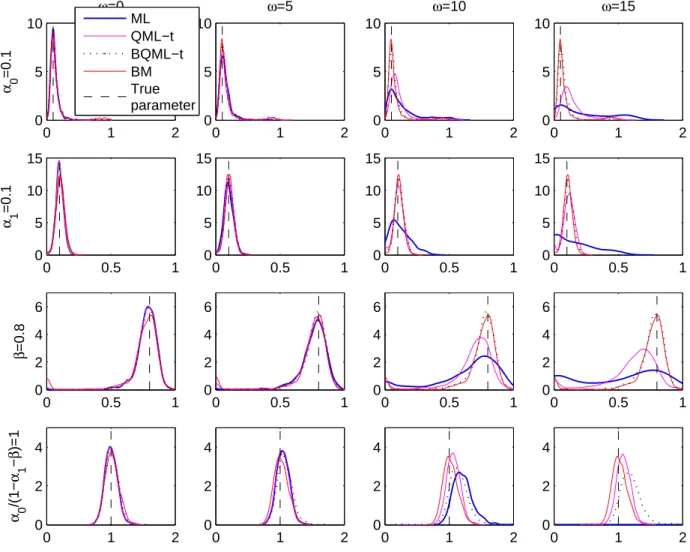
values larger or smaller respectively than the corresponding true values. Note that Table 1 reports the mean through the Monte Carlo estimates which given the shape of the densities could be rather uninformative. Observe that, in the presence of isolated LO, the standard deviations reported in Table 1 are so large that, in practice, the estimates can take any value within the admissible parameter space. In order to make this point clear, Figure 3 plots kernel density estimates, based on 1000 replicates of
Figure 3: Kernel density estimates of estimated parameters of simulated GARCH(1,1)
series of size T = 1000 contaminated with a single LO
0 1 2 0 5 10 ω=0 α 0 =0.1 0 1 2 0 5 10 ω=5 0 1 2 0 5 10 ω=10 0 1 2 0 5 10 ω=15 0 0.5 1 0 5 10 15 α 1 =0.1 0 0.5 1 0 5 10 15 0 0.5 1 0 5 10 15 0 0.5 1 0 5 10 15 0 0.5 1 0 2 4 6 β =0.8 0 0.5 1 0 2 4 6 0 0.5 1 0 2 4 6 0 0.5 1 0 2 4 6 0 1 2 0 2 4 α 0 /(1− α 1 − β )=1 0 1 2 0 2 4 0 1 2 0 2 4 0 1 2 0 2 4 ML QML−t BQML−t BM True parameter
with the marginal variance given byα0/(1−α1−β). As we can see in the graph, when
the series is contaminated by a single LO of size 10, the estimated density of αbM L
1
has a mode smaller than the true value 0.10 although its Monte Carlo mean is 0.1163
which is higher than the true value. Figure 3 also illustrates that the estimates of the unconditional variance obtained by pluging the ML estimates within the expression of the marginal variance, have a degenerate density spread all over the real line when the
outliers have a large size asω = 15.
At timeτ+ 1, the error in the estimated volatility is increased further with respect
to the error corresponding to a VO outlier. This is due to the presence of the fourth
term αbM L 1 ∞ P i=0 b βM Li(y2 τ−i−y∗ 2
τ−i) in equation (7) that takes into account the
differ-ence between the contaminated observations used to estimate the variances and the uncontaminated observations that enters the equation of the true underlying variances.
Given that y2
t−1−y∗t−21 > 0, there is transmission of the effects of LO at time τ to the
estimation of volatilities afterτ+ 1. Then, the errors tend exponentially towards their
previous mean.
These results are illustrated in Figure 4 that plots the means and MSE across replicates of the volatility errors of series simulated by the same GARCH(1,1) model
considered above and contaminated by one isolated LO at timeτ =T /2. The results
for consecutive LO are similar and, consequently, are not reported to save space. Com-paring Figures 2 and 4, we can observe that the errors corresponding to periods of time when there are not outliers have similar means in the presence of LO and VO. However, at periods of time just after the appearance of the outlier, the errors are much larger when the outliers are LO than when they are VO. Observe that the time taken by the errors to reach the level previous to the appareance of the outlier is similar in the presence of VO and LO. Furthermore, the MSE are also similar in both cases.
3
Robust estimators of the parameters
We have seen that the estimates of the underlying volatility in a GARCH(1,1) model can be seriously affected by outliers through their effect on the estimates of the pa-rameters. These effects can be mitigated by estimating the parameters using robust estimators. Sakata and White (1998) show that maximizing the likelihood based on a heavy tailed distribution is a procedure of protection against outliers when estimating the parameters of GARCH(1,1) models; see also Karanasos and Kim (2006) who sug-gest estimating the A-PARCH model using heavy tailed distributions to accommodate the presence of outliers. On the other hand, Newey and Steigerwald (1997) show that, if no outliers are present, the QML-t estimator based on maximizing the Student-t log-likelihood where the degrees of freedom are considered as an unknown parameter,
Figure 4: Monte Carlo means and MSE of ξLO
t in the presence of one isolated VO
computed with different estimators and filters in GARCH(1,1) series of size T = 1000
1 500 1000 0 0.2 0.4 Mean Error ω =0 1 500 1000 0 0.2 0.4
Mean Square Error
1 500 1000 0 0.2 0.4 ω =5 1 500 1000 0 0.2 0.4 1 500 1000 0 0.2 0.4 ω =10 1 500 1000 0 0.2 0.4 1 500 1000 0 0.2 0.4 ω =15 t 1 500 1000 0 0.2 0.4 t ML QML−t BQML−t BM zero line
is consistent and efficient when the assumed and true densities are symmetric1.
Fur-thermore, Carnero et al. (2007) show that the QML-t estimator is resistant against outliers without loosing efficiency when implemented to estimate the parameters of
ARCH models. However, it fails to be robust when estimating theβ parameter of the
GARCH(1,1) model. This lack of robustness can be explained, as Muler and Yohai (2007) pointed out, by the transmission of the effects of outliers through past condi-tional variances. Consequently, in this section we propose the BQML-t estimator which modifies the QML-t estimator by changing the specification of the conditional variance in such a way that the propagation of the outlier effect is restricted; see Muler and Yohai (2007). We derive the asymptotic distribution of the BQML-t estimator, show that the BQML-t estimator is efficient when no outliers are present in the data and has nice robustness properties when they are present. Alternatively, Muler and Yohai (2007) have recently proposed the BM robust estimator to estimate the parameters of GARCH(1,1) which is designed to deal with large number and/or large sizes of outliers. Finally, we compare the finite sample properties of the BQML-t and BM estimators
for different outlier sizes2.
3.1
BQML-t estimator
The QML-t estimator is based on maximizing the following Student-t log-likelihood
L = T X t=2 Lt= T X t=2 log Γ η+ 1 2η −log Γ 1 2η − 12 log 1−2η η + logπ + logσ2t +η+ 1 η log 1 + η 1−2η y2 t σ2 t (8)
where Γ(·) is the Gamma function and η = 1/ν where ν are the degrees of freedom
of the Student-t distribution. The parameter η can be considered as a measure of
tail thickness which always remains in the finite range 0 ≤ η < 0.5 if the conditional
distribution is restricted to have finite variance, i.e. ν > 2; see Fiorentiniet al. (2003).
If we denote by θ the vector of unknown parameters, i.e. θ = (α0, α1, β, η)′., the
BQML-t estimator is obtained as follows: 1
When this symmetry condition is not satisfied, Newey and Steigerwald (1997) show that, unless the conditional mean is identical to zero, the QML-t estimator is consistent if an additional location parameter is added to the model. Given that outliers can generate asymmetries, we also consider the introduction of this additional parameter. The modified ARCH(p) model is given by yt= (δ+εt)σt
where σ2
t = α0 +
Pp
i=1αiy
2
t−i. The results are the same as the ones obtained when δ = 0 and,
consequently, they are not reported.
2
There are also proposals of estimators based on Least Absolute Deviations (LAD); see, for example, Park (2002) and Peng and Yao (2003). However, Muler and Yohai (2007) show that their proposed BM estimator outperforms them.
b θBQM L−t= ( b θ1 if L≥L∗k b θ2 if L < L∗k (9)
whereθb1 is the parameter vector that maximizes the Student log-likelihood in (8), i.e.
b
θQM L−t, and θb
2 is the parameter vector that maximizes the modified expression of the
Student log-likelihood,L∗
k, given by (8) withσt2 substituted by
σ∗2 kt =α0+α1rk y2 t−1 σ∗2 kt−1 σ∗2 kt−1+βσ ∗2 kt−1 (10) where rk(x) = x, |x|< k
k, |x| ≥k . Muler and Yohai (2007) suggest choosing k = 5.02.
However, our simulation results suggest that, for the GARCH models usually
encoun-tered in practice,k= 9 provides a better compromise between efficiency and robustness.
The asymptotic distribution of the BQML-t estimator can be derived by following the arguments of Muler and Yohai (2007) who show that under certain regularity conditions, the asymptotic distribution of a M-estimator and the bounded M-estimator
coincide. Note that the QML-t estimator,θb1, can be expressed as a M-estimator if the
density assumed to construct the likelihood is symmetric. In particular, θb1 can be
obtained by minimizing the following objective function
M = 1 T −1 T X t=2 ρ(logyt2−logσt2)
and ρ(u) = logΓ((Γ(ν+1)ν/2)/2)+ 12log(ν−2)−u+ (ν+ 1) log 1 + νe−u2. Therefore, it
is possible to show that the asymptotic distribution of θbBQM L−t is the same as this of
b θ1 which is given by √ T(θbBQM L−t−θ)→d N(0, A−1BA−1) where A = P lim T→∞ h −T1 P∂2logL t ∂θ∂θ′ i , B = P lim T→∞ 1 T P∂logLt ∂θ ∂logLt ∂θ′
and the probability
limits are taken under the true density. When the true density is maximized A = B
and, consequently, the asymptotic covariance matrix is given by A−1 which obviously
is the asymptotic covariance matrix of the ML estimator. The asymptotic covariance
matrix of bθBQM L−t can be approximated in finite samples by
X∂2logL t ∂θ∂θ′ −1X ∂logLt ∂θ ∂logLt ∂θ′ X∂2logL t ∂θ∂θ′ −1 .
The derivatives needed to compute the covariance matrix above have been derived in the appendix.
To analyze the finite sample properties of the BQML-t estimator, we have carried out Monte Carlo experiments with the same design described above. Figures 1 and
3 plots kernel estimates of the densities of the BQML-t estimator when k = 9 and
the sample size is T = 1000, in the presence of an isolated VO and an isolated LO
respecively. For the sake of comparison, we also plot the densities of the QML-t estima-tor. Note that in the case of VO, the densities of the QML-t and BQML-t estimators
coincide. This is due to the fact that the BQML-t estimator nearly always chooses bθ1.
First, note that when ω = 0, the densities of the ML, QML-t and BQML-t
estima-tors are rather similar. Therefore, if no outliers are present in the data, the QML-t and BQML-t estimators reach a efficiency bound similar to this of the ML estimator. Second, in the presence of an isolated VO, the QML-t and BQML-t estimators have nice robustness properties. Furthermore, as we discussed before, in the presence of an
isolated LO, the QML-t estimator ofβ has a very dispersed density. However, the large
dispersion of this estimator of β is clearly reduced by the bounding mechanism
intro-duced by the BQML-t estimator. However, note that when estimating the marginal variance, the properties of the QML-t estimator are better than those of the BQML-t estimator. In this sense, the BQML-t seems to be better than QML-t in estimating each of the parameters individually but worse in estimating the unconditional variance. As we will see in Section 4, this will be important when estimating the conditional variance or volatility.
3.2
Comparison with BM estimator
Muler and Yohai (2007) propose to use M-estimators of the parameters of GARCH models. In particular, they propose the estimator, denoted as BM, which is based on the maximization of a conveniently modified likelihood and includes an additional mechanism for restricting the propagation of the effect of one outlier on the next esti-mated conditional variances as in equation (10). They show that the BM estimator is simultaneously robust against outliers and consistent when there is not contamination. Moreover, it has high efficiency.
The BM estimator of the parameters of the GARCH(1,1) model is given by
b θBM = ( b θ1, M ≤Mk∗ b θ2, M > Mk∗
whereθb1 is the argument which minimizes the following function:
M = 1 T −1 T X t=2 ρ logy2 t −logσ2t where ρ(x) = m1 h −log√1 2πexp(e
x−x)i and k = 5.02. The function m
defined by m1(x) = x, x≤4.02 c0+c1x+c2x2 +c3x3+c4x4 4.02< x≤4.3 4.16 x >4.3
where c0 = 6777, c1 =−8536.2, c3 = −379.0087 and c4 = 22.777 and the conditional
variance,σ2
t, is defined in equation (3). However, to take into account the effect of the
potential outliers on the conditional variance, it can be replaced by (10). In this case,
the modified objective function, denoted by M∗
k, is obtained and the corresponding
estimator isθb2.
To compare the finite sample properties of the BM estimator with those of the BQML-t estimator, we have carried out the same Monte Carlo experiments as before. Once more, the kernel estimates of the resulting BM estimates have been plotted in Figures 1 and 3 for isolated VO and LO, respectively. The same conclusion arises from both figures: although the densities of the BQML-t and BM estimators are very similar for the three parameters of the model, the BM densities are better behaved when estimating the marginal variances.
It is important to note that the BM estimators can be affected by the inlier problem
that appears when one observation of yt is close to zero or exactly zero. In the latter
case, it is not possible to obtain the transformation logy2
t but even in cases where yt
is close to zero, this transformation is going to take extremely large negative values. Note that this problem is of practical importance when analyzing financial returns as they can be zero when looking at returns of low traded assets; see Fuller (1996) who proposes a transformation to solve this problem.
The BQML-t estimator is simpler and has comparable finite sample properties for small samples and outlier sizes with the robust estimators proposed by Muler and Yohai (2007). Although, as expected, the BM estimator performs better when the sample size and the sizes or number of the outliers are very large, the differences between both estimators are not large for the situations usually encountered when analyzing real data. Consequently, the good robustness properties and the simplicity of the BQML-t estimator makes it an interesting candidate to be considered when trying to estimate the GARCH(1,1) parameter in series that can be potentially contaminated by outliers.
4
Estimation of the underlying volatility
As we mentioned in the Introduction, the final objective when fitting a conditional heteroscedastic model to financial returns is to obtain estimates of the underlying volatilities. We have also seen before that outliers may distort these estimates when the ML estimator is implemented. Therefore, in this section, we analyze the performance of using robust procedures to estimate both the parameters and underlying volatilities.
Once the parameters have been estimated, we have alternative options to estimate the underlying volatilities. First, as illustrated in Section 2, we can estimate them
by equation (3) where the observations, yt, are the original observations of the series
of interest and the parameters are substituted by the ML estimates based on these
observations. We have then (bσM L
t )2. Alternatively, the underlying volatilities can be
estimated by the following robust filter proposed by Muler and Yohai (2002, 2007):
b σtBM 2 =αb0BM +αbBM1 rk y2 t−1 b σBM t−1 2 ! b σtBM−1 2 +βbBM bσtBM−1 2 (11)
whererk(x) is defined as in equation (10) and the parameters are estimated by the BM
estimator.
Finally, we analyze the properties of another robust filter to estimate the volatility
given by (10) with rk(x) defined now as follows:
rk(x) =
x, |x|< k
1, |x| ≥k. (12)
Therefore, using this filter, the observations corresponding to squared standardized
observations larger than k are set equal to their conditional standard deviation.
Fur-thermore, we use the QML-t and BQML-t estimates of the parameters instead of the BM estimates. The resulting estimates of the underlying volatilities are denoted by
b σBQM L−t t 2 and bσQM L−t t 2 ,respectively.
Figure 2 plots the Monte Carlo means and MSE of the estimation errors of the conditional variances when the GARCH series are contaminated by an isolated VO. In this case, we can observe that the mean errors obtained when estimating the volatility using the filter proposed by Muler and Yohai (2007) are smaller than when using the
using the σbQM L−t t 2 and bσBQM L−t t 2
filters. On the other hand, the three robust methods have mean errors smaller in absolute value than the mean errors of the ML filter. When looking at the MSE, it is possible to observe that they are similar among the three robust filters and smaller than the MSE of the ML filter.
Also, it is interesting to note that the mean errors incurred by the robust filters are negative and large in the moment when the outlier appears. This is due to the fact that when computing the robust filters, the large observations are cut down, generating in the next period an estimate of the underlying volatility smaller than it should be. Therefore, although the robust filters considered in this paper have in any case better properties than the ML filters, they are not properly designed to deal with VO.
Figure 4 plots the same quantities plotted in Figure 2 when the series are contami-nated by LO. As before, the filter with smaller mean errors in the periods of time when there are no outliers is the BM filter followed by the QML-t and BQML-t filters. The mean errors of the ML filter are clearly larger. On the other hand, the MSE errors of
the three robust filters are clearly smaller than for the ML filter. Furthermore, in this case, the mean errors of the robust filters corresponding to the periods of time around the appearance of the outliers are positive and clearly smaller when using the function
rk(x) as defined in (12) instead of the definition in (10).
Therefore, these results suggest that, although the properties of the BQML-t esti-mator are better than those of the QML-t estiesti-mator, the estimates of the underlying volatilities have better properties when using the robust filters using the QML-t es-timates of the parameters. As mentioned before, this could be explained by the way the marginal variance is estimated. Intuition does not work here, since one tends to think that good parameter estimates lead to good volatility estimates; see, for ex-ample, Charles and Darn´e (2006) for this kind of conclusion. However we should be careful when considering ”good” estimators. As a simple example, consider the GARCH(1,1) model of the Monte Carlo experiments, i.e. with true parameter values
θ = (α0, α1, β) = (0.1,0.1,0.8). The true marginal variance of this process is 1.
Sup-pose we have two estimators ˜θ1 and ˜θ2 which, for a particular series, give estimates
of the parameters equal to (0.02,0.08,0.9) and (0.11,0.099,0.85) respectively. Clearly,
˜
θ2 gives estimates which are closer to the true θ. However, estimates given by ˜θ1 are
closer to the true marginal variance. Therefore, it is expected that ˜θ1 lead to better
estimates of the volatility in spite of not being as close toθ as ˜θ2.
We have also seen that when using the robust filters, it is better to use the definition
of the rk(x) function when the large observations are set equal to their conditional
standard deviations. Also, between the robust filters, the one with smallest mean errors is obtained when using the BM estimates of the parameters. However, the alternative filter based on using the QML-t estimates is a good compromise between simplicity and mean errors. Furthermore, all the robust methods have similar MSE which are clearly smaller then those of the ML filter. Finally, the fourth conclusion is that the robust filters are not well designed to deal with VO. Therefore, it seems of interest to design procedures to detect outliers that differentiate whether an outlier is VO or LO. The filters needed to estimate the variances in each of these cases should be different.
5
Empirical application
This section illustrates the advantages of using robust estimates of the conditional variance when a GARCH(1,1) model is fitted to daily returns of the S&P500 and the
IBEX35 indexes3observed from January 2, 1987 to February 19, 2008 and from January
2, 1995 to February 20, 2008 respectively. Figure 5 plots both series of prices and the corresponding returns. The volatility clustering observed in the returns series suggests the presence of conditional heteroscedasticity which we model by fitting a GARCH(1,1)
3
Figure 5: Daily prices and returns for S&P500 and IBEX35
02−Jan−19870 30−Jan−1998 19−Feb−2008 500
1000 1500
S&P 500
02−Jan−19950 21−March−2002 20−Feb−2008 5000
10000 15000
IBEX 35
03−Jan−1987 02−Feb−1998 20−Feb−2008 −20 −15 −10 −5 0 5 10 Returns
03−Jan−1995−10 22−March−2002 20−Feb−2008 −5
0 5 10
model to each of the series. The corresponding ML estimates appear in Table 2. In
both series, the persistence is estimated very close to one with αb1 +βb = 0.99. On
the other hand, the plug-in variances obtained when the estimated parameters are substituted in the expression of the marginal variance of a GARCH(1,1) model, i.e.
α0/(1−α1−β), are given by 1.45 and 2.06 respectively.
Visual inspection of the plots of returns in Figure 5 shows that outliers could be present in both series. Consequently, in order to avoid potential biases caused by these observations, we estimate GARCH parameters and volatility using robust methods. Table 2 also contains estimates of the parameters obtained by using the estimators:
QML-t, BQML-t withk = 9 and BM with k = 5. As we can see in the Table, for both
series, the constant α0 and also the ARCH parameter α1 are overestimated while β is
underestimated when using ML compared to robust methods. Notice that, for these particular two series, the BQML-t estimator gives exactly the same estimated values for the parameters as QML-t. This is because the likelihood function is not higher when the effect of big observations is truncated in the variance equation and therefore the estimator coincides with QML-t as equation (9) shows. On the other hand, the estimates obtained when using the BM estimator are similar to those obtained by the QML-t estimator with the BM estimate of the ARCH parameter being slightly larger when fitting the GARCH model to the S&P500 returns and slightly smaller in the IBEX35 returns. The persistence estimated is also very close to one and similar to those estimated by ML. Notice that the plug-in marginal variances of S&P500 estimated
by the QML-t and BM estimators are 1.32 and 0.53 respectively while those of the
IBEX35 returns are 2.71 and 1.01. Finally, note that the QML-t estimated degrees of
freedom are 6.30 and 9.51 for the S&P500 and IBEX35 returns respectively. The fact
that the estimated degrees of freedom are far from suggesting a conditionally Normal distribution can be attributed to the presence of outliers.
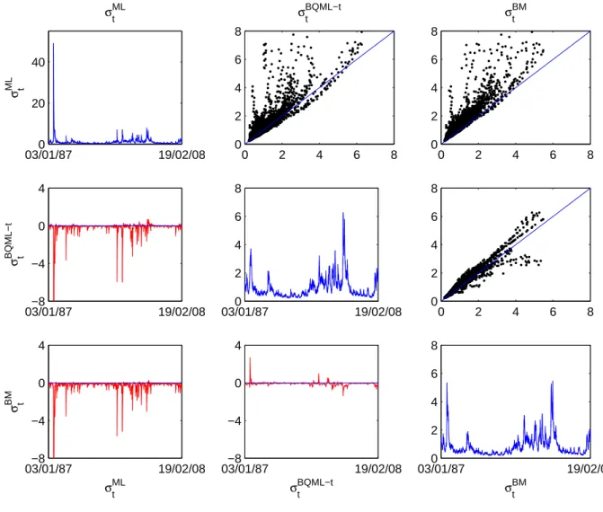
Estimated GARCH volatilities for both S&P500 and IBEX35 return series are plot-ted in Figures 6 and 7 respectively. The diagonal of the picture contains estimaplot-ted
GARCH volatility, σ2
t, using the four alternative estimators: ML, QML-t, BQML-t
and BM each with its corresponding filter for the variance as explained above. As we have discussed before, for these particular series, BQML-t and QML-t produce exactly the same estimations and therefore just one of them, BQML-t, is considered. The plots above the diagonal are scatter plots of the estimated volatilities using each of the methods. For example, the graph in the first row and third column of Figures 6 and
7 is the scatter plot of (σbBM
t )2 (which is bσt2 calculated using the BM estimator of the
parameters and the robust filter as given in equation (11)) against (bσM L
t )2 (which is bσ2t
obtained by using the ML estimator of the parameters and the usual variance equation as given in equation (4)). The plots below the diagonal contain the difference between estimated conditional variances using each of the methods. As an example, the graph in the second row and first column of Figures 6 and 7 plots the time series computed
Figure 6: Estimated volatility ˆσ2
t, scatter-plot of different estimated volatilities and
difference between estimated volatilities for the S&P500
03/01/870 19/02/08 20 40 σ ML t σML t 0 2 4 6 8 0 2 4 6 8 σBQML−t t 0 2 4 6 8 0 2 4 6 8 σBM t 03/01/87−8 19/02/08 −4 0 4 σ BQML−t t 03/01/870 19/02/08 2 4 6 8 0 2 4 6 8 0 2 4 6 8 03/01/87−8 19/02/08 −4 0 4 σML t σ BM t 03/01/87−8 19/02/08 −4 0 4 σBQML−t t 03/01/870 19/02/08 2 4 6 8 σBM t
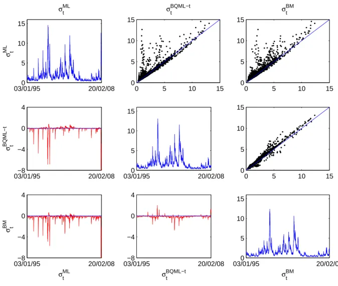
Figure 7: Estimated volatility ˆσ2
t, scatter-plot of different estimated volatilities and
difference between estimated volatilities for the IBEX35
03/01/950 20/02/08 5 10 15 σ ML t σML t 0 5 10 15 0 5 10 15 σBQML−t t 0 5 10 15 0 5 10 15 σBM t 03/01/95−8 20/02/08 −4 0 4 σ BQML−t t 03/01/950 20/02/08 5 10 15 0 5 10 15 0 5 10 15 03/01/95−8 20/02/08 −4 0 4 σML t σ BM t 03/01/95−8 20/02/08 −4 0 4 σBQML−t t 03/01/950 20/02/08 5 10 15 σBM t
as (bσBQM L−t
t )2 -(bσtM L)2 .
It is clear that ML tends to overestimate volatility compared to robust methods. This is shown in the pictures for both series. By looking at the scatter plots in the first raw, we can see that most of the points are above the 45 degrees line, meaning that
values in the X-axis are smaller than values in the Y-axis ((σbM L
t )2). The same
conclu-sion can be obtained by looking at the plots in the first column. Most of these values
are negative meaning that (bσM L
t )2 is larger than any of the other robust estimations.
This is expected when outliers are present in the data, as we have shown in the paper. Notice also that robust estimations are very similar.
We have carried out a forecasting exercise in order to show the practical advantages of using robust methods when computing 95% prediction intervals for the returns.
First, we took all data available for both indexes, T = 5328 for the S&P500 and
T = 3293 for the IBEX35. With the estimated values of the parameters and the
estimated conditional variance we computed up to 15-steps-ahead forecasts for the
conditional variance, bσ2
T+1, bσ2T+2, ..., bσ2T+15 and also the corresponding 95% prediction
intervals given by±1.96bσT+1,±1.96σbT+2, ...,±1.96bσT+15. The results are shown in the
first row of Figure 8. The solid-thicker line corresponds to those intervals computed
using (bσM L
t )2, the solid-thinner line corresponds to those intervals computed using
(σbBQM L−t
t )2, which is identical to the ones corresponding to (bσQM Lt −t)2 and finally, the
dotted line corresponds to intervals computed using (bσBM
t )2. The second row of this
figure contains the results of a similar exercise with different samples for both indexes. For the S&P500 we took data from January 2, 1987 to December 14, 1990 and from January 13, 2003 to February 20, 2008 for the IBEX 35. The choice of those particular samples was done in order to take moderate sample sizes, around 1000 observations, and having possible outliers in the data.
Three main conclusions can be obtained by looking at Figure 8. First, prediction intervals based on ML are, in general, wider than the ones based on robust methods. This was expected given that, as illustrated before, ML tends to overestimate the conditional variance. Second, differences among ML and robust methods are very
small in large sample sizes as we can see in the plot for the S&P500 whenT = 5328. In
this case, the three prediction intervals are practically the same. However, differences are not negligible in smaller sample sizes. And last, robust methods give very similar results for both series and all sample sizes considered.
6
Conclusions
Detecting outliers in conditional heteroscedastic time series is a difficult task, and es-timating the underlying volatilities without taking into account their presence may
be very misleading. We have shown in this paper that biased estimators of the
Figure 8: Prediction intervals for the returns of S&P500 and IBEX 35 together with actual values with two different samples
08−Jan−2008 11−Mar−2008 −4
0 4
Sample size 5328
Returns and 95% prediction intervals for S&P 500
09−Jan−2008−8 12−Mar−2008 −4 0 4 8 Sample size 3293
Returns and 95% prediction intervals for IBEX 35
09−Nov−1990 03−Jan−1991 −4 0 4 Sample size 1000 09−Jan−2008−8 12−Mar−2008 −4 0 4 8 Sampel size 1293 ML BQML−t BM Actual value
non linear way, so that having small biases in the estimated parameters is not a guar-antee of small biases in estimated volatilities. Therefore, it seems a good strategy to estimate the parameters of the model and the underlying volatilities using robust methods. We show the performance of three robust estimators and two robust filters in modeling time series which contain both outliers and conditional heteroscedasticity. The three estimators, QML-t, BQML-t and BM with their corresponding filters have good properties with no outliers and they are better than ML when outliers are present in the data.
Acknowledgments
Financial support from project SEJ2005-02829/ECON by the Spanish Government is gratefully acknowledged. Thanks to the participants at the ESEM07 meeting in Bu-dapest and Simposio de An´alisis Econ´omico in Granada and at seminars at Universidad de Alicante, Universidad Complutense de Madrid and Universidad Carlos III de Madrid for helpful comments and suggestions. We are also very grateful to the comments of one anonymous referee that have improved this paper. Any remaining errors are our own.
Appendix. Derivatives needed to compute the
asymp-totic covariance matrix of the QML-t estimator of
the GARCH(1,1) model
The asymptotic distribution of the QML-t estimator is given by
√ T(θb−θ)→d N(0, A−1BA−1) where A = P lim T→∞ h −T1 P∂2logL t ∂θ∂θ′ i and B = P lim T→∞ 1 T P∂logLt ∂θ ∂logLt ∂θ′
where the prob-ability limits are taken under the true density. When the true density is maximized
A = B and, consequently, the asymptotic covariance matrix is given by A−1 which
obviously is the asymptotic covariance matrix of the ML estimator. The asymptotic
covariance matrix of bθ can be approximated in finite samples by
X∂2logL t ∂θ∂θ′ −1X ∂logL t ∂θ ∂logLt ∂θ′ X∂2logL t ∂θ∂θ′ −1
The Student-t log-likelihood of the GARCH(1,1) model is given by
logLt= log Γ η+ 1 2η −log Γ 1 2η −0.5 log 1−2η η −0.5 log [π]− −0.5 logσt2− η+ 1 2η log 1 + η 1−2ηε 2 t whereσ2 t =α0+α1yt2−1+βσt2−1 and ε2t =yt2/σt2.
First order derivatives:
∂logLt ∂α0 =− 1 2σ2 t ∂σ2 t ∂α0 1−2η−ε2 t 1−2η+ηε2 t ∂logLt ∂α1 =− 1 2σ2 t ∂σ2 t ∂α1 1−2η−ε2 t 1−2η+ηε2 t ∂logLt ∂β =− 1 2σ2 t ∂σ2 t ∂β 1−2η−ε2 t 1−2η+ηε2 t ∂logLt ∂η = 1 2η 1 1−2η − 1 η ψ η+ 1 2η −ψ 1 2η −log 1 + η 1−2ηε 2 t −
(η+ 1)ε2 t
(1−2η)(1−2η+ηε2
t)
whereψ(·) is the digamma function and
∂σ2 t ∂α0 = 1−β t−1 1−β + βt−1 1−α1−β ∂σ2 t ∂α1 = t−2 X i=0 βiyt2−1−i+βt−1 σ 2 y 1−α1−β ∂σ2 t ∂β = t−2 X i=0 βiσt2−1−i+βt−1 σ 2 y 1−α1−β whereσ2 1 =σy2 = 1−αα10−β.
Second order derivatives:
∂2logLt ∂α2 0 = 1 2σ4 t ∂σ2t ∂α0 2 1−2η−ε2t 1−2η+ηε2 t − 1−η−2η2 (1−2η+ηε2 t)2 ε2t ∂2logL t ∂α0∂α1 = 1 2σ2 t 1 1−2η+ηε2 t 1 σ2 t ∂σ2 t ∂α0 ∂σ2 t ∂α1 1−2η−ε2t − 1−η−2η2 1−2η+ηε2 t ε2t − ∂ 2σ2 t ∂α0∂α1 (1−2η−ε2t) ∂2logL t ∂α0∂β = 1 2σ2 t 1 1−2η+ηε2 t 1 σ2 t ∂σ2 t ∂α0 ∂σ2 t ∂β 1−2η−ε2t − 1−η−2η 2 1−2η+ηε2 t ε2t − ∂ 2σ2 t ∂α0∂β (1−2η−ε2t) ∂2logL t ∂α0∂η = 1 2σ2 t ∂σ2 t ∂α0 ε2 t(3−ε2t) (1−2η+ηε2 t)2 ∂2logL t ∂α2 1 = 1 2σ2 t 1 1−2η+ηε2 t " 1 σ2 t ∂σ2 t ∂α1 2 1−2η−ε2t − 1−η−2η 2 1−2η+ηε2 t ε2t − ∂ 2σ2 t ∂α2 1 (1−2η−ε2t) # ∂2logL t ∂α1∂β = 1 2σ2 t 1 1−2η+ηε2 t 1 σ2 t ∂σ2 t ∂α1 ∂σ2 t ∂β 1−2η−ε2t − 1−η−2η 2 1−2η+ηε2 t ε2t − ∂ 2σ2 t ∂α1∂β (1−2η−ε2t) ∂2logL t ∂α1∂η = 1 2σ2 t ∂σ2 t ∂α1 ε2 t(3−ε2t) (1−2η+ηε2 t)2
∂2logL t ∂β2 = 1 2σ2 t 1 1−2η+ηε2 t " 1 σ2 t ∂σ2 t ∂β 2 1−2η−ε2 t − 1−η−2η2 1−2η+ηε2 t ε2 t −∂ 2σ2 t ∂β2 (1−2η−ε 2 t) # ∂2logL t ∂β∂η = 1 2σ2 t ∂σ2 t ∂β ε2 t(3−ε2t) (1−2η+ηε2 t)2 ∂2logL t ∂η2 = 4η−1 2η2(1−2η)2 + 1 η3 ψ η+ 1 2η −ψ 1 2η −log 1 + η 1−2ηε 2 t −41η4 ψ′ 1 2η −ψ′ η+ 1 2η + ε 2 t 2η(1−2η)(1−2η+ηε2 t) 2 η + (η+ 1)(ε2 t −2) (1−2η+ηε2 t) − 2(η+ 1) (1−2η) where ∂2σ2 t ∂α0∂α1 = β t−1 (1−α1−β)2 ∂2σ2 t ∂α0∂β = 1 +β t−2(1−2β−t+tβ) (1−β)2 + βt−2[(t−1)(1−α 1−β) +β] (1−α1−β)2 ∂2σ2 t ∂α2 1 = 2α0β t−1 (1−α1−β)3 ∂2σ2 t ∂α1∂β = t−1 X i=1 iβi−1y2 t−1−i+ α0βt−2((t−1)(1−α1−β) + 2β) (1−α1−β)3 ∂2σ2 t ∂β2 = t−2 X i=1 iβiσt2−1−i+ t−2 X i=0 βi∂ 2σ2 t−1−i ∂β2 +βt−2 σ 2 y (1−α1 −β)2 [(t−1)(1−α1−β) + 2β] where ∂2σ21 ∂β2 = 2σ2 y (1−α1−β)2.
References
[1] Carnero, M.A., D. Pe˜na and E. Ruiz (2007), Effects of outliers on the identification
and estimation of GARCH models. Journal of Time Series Analysis, 28(4),
471-497.
[2] Charles, A. and O. Darn´e (2006), Large shocks and the September 11th terrorist
attacks on international stock markets.Economic Modelling, 23, 683-698.
[3] Bollerslev, T. (1987), A conditional heteroskedastic time series model for
specula-tive prices and rates of return.Review of Economics and Statistics, 69, 542-547.
[4] Doornik, J. and Ooms, M. (2004), Outlier Detection in GARCH Models, Mimeo, Nuffield College. University of Oxford.
[5] Fiorentini, G., Sentana, E., Calzolari, G. (2003), Maximum likelihood estima-tion and inference in multivariate condiestima-tionally heteroskedastic dynamic regression
models with Student-t innovations. Journal of Business and Economic Statistics
21, 532546.
[6] Fuller, W.A. (1996), Introduction to Statistical Time Series, Wiley, New York.
[7] Grossi, L. (2004), Analyzing financial time series through robust estimators.
Stud-ies in Nonlinear Dynamics& Econometrics, 8(2).
[8] Hotta, L.K. and Tsay, R.S. (1998), Outliers in GARCH processes, Mimeo, Uni-versity of Chicago.
[9] Muler, N. and V. Yohai (2002), Robust estimates for ARCH processes. Journal of
Time Series Analysis,23, 341-375.
[10] Muler, N. and V. Yohai (2007), Robust estimates for GARCH models.Journal of
Statistical Planning and Inference.Forthcoming.
[11] Karanasos, M. and J. Kim (2006), A re-examination of the asymmetric power
ARCH model.Journal of Empirical Finance, 13, 113-128.
[12] Newey, W.K. and Steigerwald, D.G. (1997), Asymptotic bias for
quasi-maximum-likelihood estimators in conditional heteroskedasticity models. Econometrica 65,
587-99.
[13] Park, B. (2002), An outlier robust GARCH model and forecasting volatility of
exchange rate returns,Journal of Forecasting, 21, 381-393.
[14] Peng, L. and Q. Yao (2003), Least absolute deviations estimation for ARCH and
[15] Sakata, S. and H. White, 1998, High breakdown point conditional dispersion
es-timation with application to S&P500 daily returns volatility, Econometrica, 66,
529-567.
[16] Van Dijk, D., Franses, P.H. and A. Lucas, 1999, Testing for ARCH in the presence