Deconstructing Hardware Usage for General Purpose Computation on GPUs
Budyanto Himawan
Dept. of Computer Science University of Colorado
Boulder, CO 80309
Manish Vachharajani
Dept. of Electrical and Computer Engineering University of Colorado
Boulder, CO 80309
E-mail:
{
Budyanto.Himawan,manishv
}
@colorado.edu
Abstract
The high-programmability and numerous compute resources on Graphics Processing Units (GPUs) have allowed researchers to dramatically accelerate many non-graphics applications. This initial success has generated great interest in mapping applica-tions to GPUs. Accordingly, several works have focused on help-ing application developers rewrite their application kernels for the explicitly parallel but restricted GPU programming model. How-ever, there has been far less work that examines how these appli-cations actually utilize the underlying hardware.
This paper focuses on deconstructing howGeneral Purpose ap-plications on GPUs (GPGPU apap-plications) utilize the underlying GPU pipeline. The paper identifies which parts of the pipeline are utilized, how they are utilized, and why they are suitable for general purpose computation. For those parts that are utilized, the paper examines the underlying causes for the under-utilization and suggests changes that would make them more use-ful for GPGPU applications. Hopeuse-fully, this analysis will help de-signers include the most useful features when designing novel par-allel hardware for general purpose applications, and help them avoid restrictions that limit the utility of the hardware. Further-more, by highlighting the capabilities of existing GPU compo-nents, this paper should also help GPGPU developers make more efficient use of the GPU.
1.
Introduction
In recent years, CPU performance growth has slowed and this slowing seems likely to continue [1]. Thus, designers are looking to other means to boost application performance; explicitly par-allel hardware, especially non-traditional parpar-allel hardware (e.g., IBM’s Cell Processor), is a top choice. To understand how to best design non-standard architectures, Graphics Processing Units (GPUs) can provide an interesting lesson. GPUs allow highly parallel (though mostly vectorized) computations at relatively low cost. Furthermore, the relatively simple parallel architecture of the GPU allows the performance of these designs to scale as Moore’s law provides more transistors. As evidence, consider that GPU performance has been increasing at a rate of 2.5 to 3.0x annually as opposed to 1.41x for general purpose CPUs [2].
Although older GPUs tend to sacrifice programmability for
performance, in 2001, NVidia revolutionized the GPU by making it highly programmable [3]. Since then, the programmability of GPUs has steadily increased, although they are still not fully gen-eral purpose. Since this time, there has been much research and ef-fort in porting both graphics and non-graphics applications to use the parallelism inherent in GPUs. Much of this work has focused on presenting application developers with information on how to perform the non-trivial mapping of general purpose concepts to GPU hardware so that there is a good fit between the algorithm and the GPU pipeline.
Less attention has been given to deconstructing how these gen-eral purpose application use the graphics hardware itself. Nor has much attention been given to examining how GPUs (or GPU-like hardware) could be made more amenable to general purpose com-putation, while preserving the benefits of existing designs. In this paper, we investigate both of these aspects of General Purpose ap-plications on GPUs (GPGPU). We use the taxonomy of funda-mental operations (mapping, sorting, reduction, searching, stream filtering, and scattering and gathering) developed by Owens et al. [4] to examine how GPGPU applications utilize GPU hardware. We describe how each operation can be implemented on the GPU, identify which hardware components are used, how they are used, and why they are suitable for general purpose applications. This should help designers determine which features to keep or improve and which limitations to avoid in the design of the next generation GPUs to make them more useful for general purpose computa-tion. Furthermore, by highlighting the capabilities and limitations of existing GPU components, this paper should also help devel-opers build more efficient GPGPU applications. As a step in this direction, this work also extends Owens et al. with a new funda-mental operation,predicate evaluation.
The remainder of this paper is organized as follows. Section 2 provides an overview of the GPU architecture and shows the map-ping between GPU and general purpose computing concepts by showing how a simple vector scaling operation is implemented. Section 3 examines the fundamental operations, describes how they can be implemented on the GPU, and identifies the pieces of GPU hardware that are utilized. In Section 4, we provide a summary of the capabilities and limitations of the different pieces of the GPU hardware and suggests a few modifications. This anal-ysis can serve as the basis for further investigations into GPU ex-tensions for GPGPU computation. Section 5 concludes.
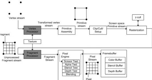
Figure 1. Overview of a GPU Pipeline. Shaded boxes represent programmable components
2.
GPU Architecture Overview
This section introduces the GPU pipeline with NVidia GeForce 6800 as a model. The graphics pipeline (See Figure 1) is tradition-ally structured as stages of computation with data flow between the stages [4]. This fits nicely into the streaming programming model [5], in which, input data is represented as streams. Kernels then perform computations on the streams at different stages of the pipeline. More formally, astreamis a collection of records requir-ing similar computations and akernelis a function applied to each element of the stream [6]. We can roughly think of GPUs as SIMD machines under Flynn’s taxonomy of computer architectures [7].
The stages in the graphics pipeline are as follows:
Vertex Processor The vertex processor receives a stream of ver-tices from the application and transforms each vertex into screen positions. It also performs other functions such as generating texture coordinates and lighting the vertex to de-termine its color. Each transformed vertex has a screen po-sition, a color, and a texture coordinate. Traditional vertex processors do not have access to textures. This is a new fea-ture in the GeForce 6800.
Primitive assembly During primitive assembly, the transformed vertices are assembled into geometric primitives (triangles, quadrilaterals, lines, or points).
Cull/Clip/Setup The stream of primitives then passes through the Cull/Clip/Setup units. Primitives that intersect theview frus-tum(view’s visible region of 3D space) are clipped. Prim-itives may also beculled(discarded based on whether they face forward or backward).
Rasterizer This unit determines which screen pixels are covered by each geometric primitive, and outputs a corresponding
fragment for each pixel. Each fragment contains a pixel location, depth value, interpolated color, and texture coor-dinates. The z-cull unit attached to the rasterizer performs
early culling. The idea is to skip work for fragments that are not going to be visible to begin with.
Fragment Processor A function is applied to each fragment to compute its final color and depth. The value of a frag-ment’s color is what is normally used as the final value in a GPGPU computation. The fragment processor is also capa-ble oftexture-mapping, a process where an image is added to a simple shape, like a decal pasted to a flat surface. This feature can be used to assign a color to each fragment. The color for each fragment is obtained by performing a lookup into a 2D image (called atexture) using the fragment’s tex-ture coordinates. Each element in a texture is called a tex-ture element (texel). As we will see, texture mapping is one of the key GPU features used in GPGPU applications.
Raster Operations (Pixel engine) The stream of fragments from the fragment processor goes through a series of tests, namely thescissor, alpha, depth, andstencil test. If they survive these tests, they are written into the framebuffer. The scis-sor testrejects a fragment if it lies outside a specified sub-rectangle of the framebuffer. The alpha test compares a fragment’s alpha (transparency) value against a user spec-ified reference value. Thestencil testcompares the stencil value of a fragment’s corresponding pixel in the framebuffer with a user specified reference value. The stencil test is used to mask off certain pixels. Thedepth testcompares the depth value of a fragment with the depth value of the correspond-ing pixel in the framebuffer. Values in the depth buffer and stencil buffer can optionally be updated for use in the next rendering pass.
The pixel engine is also responsible for performing blend-ingoperations. During blending, each fragment’s color is blended with the pre-existing color of its corresponding pixel in the framebuffer. The GPU supports a wide variety of user-controlled blending operations, including conditional assignments.
Framebuffer Theframebufferconsists of a set ofpixels(picture elements) arranged in a two dimensional array [8]. It stores the pixels that will eventually be displayed on the screen. It is made up of several sub buffers, namely color, stencil, and depth buffer.
Figure 2. Block diagram of the GeForce 6 se-ries architecture.
Figure 2 (from reference [9]) shows a block diagram of a typ-ical GPU pipeline (in this case, the Nvidia GeForce 6800). There are 6 vertex processors and 16 fragment processors capable of per-forming 32 bit floating point operations. They both use the texture unit as a random access data fetch-unit at a rate of 35GB/sec [9]. The texture unit is writable and readable by both the GPU and CPU. The peak texture download and read back rate is 3.2 GB/sec. The vertex and fragment processors are fully programmable. They can execute user-programmed computation kernels, calledshaders. From here on, the terms shader, kernel, and program are used in-terchangeably.
2.1
Mapping GPU to general purpose computing
concepts
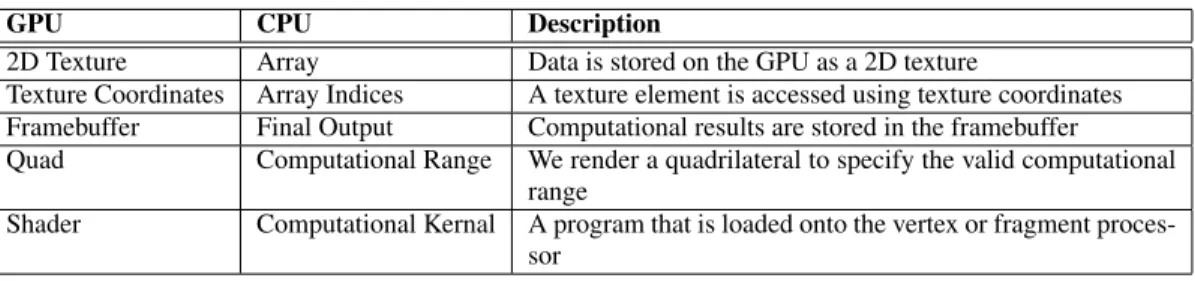
To see how the GPU can be used to perform a general purpose computation, we consider an example in which we perform vector scaling using the Cgshading language. Table 1 summarizes the GPU terms used in the example and how they map back to general purpose computing terms.
To program the GPU one has to use a 3D library to interface with the graphics hardware and ashading languageto program the GPU. The 3D interface library (e.g., Direct3D [10] or OpenGL [8]) is beyond the scope of this paper. Shading languagesenable pro-grammers to use a higher level C-like language instead of GPU assembly. High Level Shading Language (HLSL), OpenGL [11], and Cg [12] are three of the more popular shading languages. There are also extensions to general purpose languages that pro-vide abstractions to the parallel data structure of the GPU. [6, 13] provides such abstractions for C++, and [14] for C#. A compiled shader is transferred to the GPU using the appropriate 3D library commands (see Figure 3).
2.2
The vector-scaling example
Avector scalingoperation is defined asy=αx, whereyand
xare vectors of the same length. We are multiplying each element ofxby a constant,α, and storing the results in vectory. Figure 3
Figure 3. Dataflow for vector scaling on the GPU
1 float2 multiplier (
2 in float2 coords : TEXCOORD0,
3 uniform samplerRECT textureData,
4 uniform float alpha ) : COLOR {
5 float2 data = texRECT (textureData, coords); 6 return (data * alpha);
7 }
Figure 4. Cg program for vector scaling. shows the dataflow diagram of the execution of the vector scaling program. The application first allocates a 1D array on the CPU memory. This is then converted to a 2D texture and transferred to the GPU memory using OpenGL commands. Next, the Cg pro-gram is compiled by the Cg Runtime and transferred into the frag-ment processor. Computation is started byrenderingaquadthat is the size of the texture, specifying the four vertices and their associ-atedtexture coordinates. A quad specifies the computational range and usually corresponds to the size of the output. Texture coordi-nates are to textures as array indices are to arrays. They are used as lookup indices. Rendering generates a stream of vertices that be-come the input to the GPU pipeline. The rasterizer then generates fragments (along with texture coordinates) which are used by the fragment processor. Our shader performs a 2D lookup into the tex-ture using the textex-ture coordinates that arrive with each fragment. Each value obtained from the texture is multiplied by the scaling factor and the output is written into the framebuffer. Note that this multiplication is a vector operation. The results are then read-back into the CPU memory from the framebuffer. Mapping the terms back to the vector scaling equation,y=αx, theframebufferisy, the texture isx.αis passed in as a uniform parameter, which will be explained shortly.
The Cg program that performs the computation is shown in Figure 4. Compare that with the CPU version (Figure 5). Notice that the Cg program does not have a loop. The scaling operation is performed on every fragment of the incoming stream. The frag-ment processors execute as many of them in parallel as hardware resources allow.
The details of Cg are beyond the scope of this paper and read-ers are encouraged to refer to [12] for a tutorial. In summary, the
1 for (int i=0; i<lengthOf(data); i++) 2 {
3 result[i] = data[i] * alpha;
4 }
GPU CPU Description
2D Texture Array Data is stored on the GPU as a 2D texture
Texture Coordinates Array Indices A texture element is accessed using texture coordinates Framebuffer Final Output Computational results are stored in the framebuffer Quad Computational Range We render a quadrilateral to specify the valid computational
range
Shader Computational Kernal A program that is loaded onto the vertex or fragment proces-sor
Table 1. Mapping of GPU terminology to general purpose computing terminology.
Cg program performs a texture lookup using thetexRECT rou-tine.textureDatarefers to the texture (x) andcoordsrefers to texture-coordinates. Theuniformvariable qualifier indicates that the variable is fixed. They do not vary per fragment and are stored in constant registers.
3.
GPU Hardware Utilization
In this section we deconstruct how GPGPU applications utilize the underlying hardware. Owens et al. [4] identified a list of fun-damental operations that can be performed on the GPU based on the streaming programming model;mapping, reduction, sorting, searching, scattering and gathering,and stream filtering. Their work was targeted towards application developers. Here, we dis-cuss the low-level implications of these fundamental operations and how the hardware supports them. We have also identified a new operation,predicate evaluation, that was not in the original classification.
3.1
Mapping
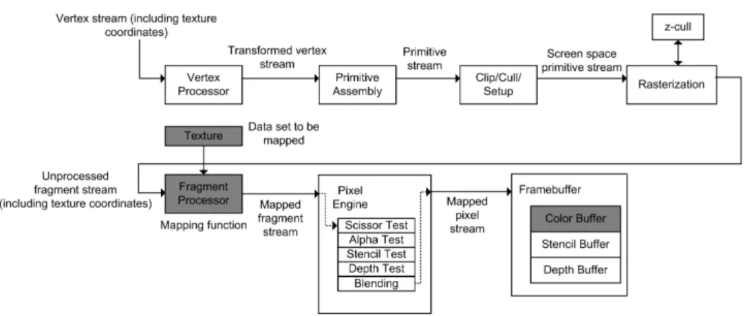
This is just like the vector scaling example in Section 2.2. Given a function and a stream, themappingoperation applies the function to each element in the stream in parallel. On a CPU pro-gram, one would have an inner loop to apply the operation on every element of a vector to achieve the same effect. With the GPU, it is as if this inner loop is unrolled and executed in parallel (as long as hardware resources are available). The pipeline usage is shown in Figure 6.
The GPU implementation for the mapping operation is straight-forward. The vector on which the mapping function is to operate is transferred to the texture unit as a 2D array. The mapping function itself is written as a fragment shader. The results are then written into the color buffer portion of the framebuffer.
Mapping operation is a very common data parallel operation. The vector scaling operation discussed in section 2.1 is a classic example. Discrete Cellular Automata used in physics simulation can be modeled using a mapping operation [15].
3.2
Reduction
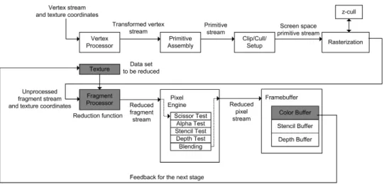
Reductionis a process where, given an input stream, one com-putes a smaller stream or even a single value. On the GPUs, re-ductions are implemented by alternately rendering to and reading from a pair of textures. This gives us a running time of O(logn) compared to O(n) on the CPU. On each rendering pass, the size of the output is reduced by some fraction. We keep doing this until the output is a single element buffer. For example to reduce a 2D buffer, the fragment program reads four elements from the input texture using four sets of texture coordinates. The output size is halved in each dimension at each step.
Figure 7 shows the typical reduction scheme used by GPGPU applications. From the application, we specify the computational range by drawing a quad and specifying the vertices. In this case our computational range would be the size of the output buffer. So the four vertices are (0,0), (2,0), (0,2), (2,2). Recall that texture coordinates are simply used by the fragment program as indices into a texture. For each vertex, we can specify a set of texture coordinates (GeForce 6800 allows up to 16).
different from the map operation, except now we perform mul-tiple rendering passes. The output buffer of one rendering pass becomes the input texture of the next pass. We leave the task of re-computing the size of the output buffer and the texture coordi-nates between rendering passes to the application.
The rasterizer linearly interpolates the coordinates at each ver-tex to generate a set of coordinates for each fragment. The in-terpolated coordinates are then passed as inputs to the fragment processor. The reduction function, which is implemented as frag-ment shader, thus takes in four texture coordinates as inputs and applies the reduction operation between corresponding texture co-ordinates. The application simply specifies the texture coordinates associated with each vertex. For example, in Figure 7, the tex-ture coordinates associated with vertex (0,0) are (0,0) for domain 0, (2,0) for domain 1, (0,2) for domain 2, and (2,2) for domain 3. Note, to avoid GPU to CPU data transfers, the successive render-ing passes are done completely in the GPU by havrender-ing the fragment program write its output to another texture, instead of writing di-rectly to the framebuffer.
The pipeline usage (Figure 8) is really no
Reduction, like mapping, is used in many applications. Ex-amples of common reduction operations are computing the max-imum, minmax-imum, or the sum from a set of values. In parallel re-ductions, the reduction operation needs to be associative so that the underlying parallel system can perform them in any order best suited for the system.
3.3
Sorting
Sortingis one of the most fundamental problems in computer science. Studies have shown that the performance of sorting algo-rithms on CPUs is limited by cache misses [16] and instruction de-pendencies [17]. This makes the GPU, which has a high memory bandwidth (up to 35 GB/sec for GeForce 6800) and a high degree of parallalelism in their fragment processors, a perfect candidate for improving sort performance.
However, classic sorting algorithms like quicksort do not nat-urally port to the GPU. They are data-dependent and they require scatter operations. To avoid write-after-read (WAR) hazards be-tween multiple fragment processors, current graphics processors do not support scatter operations from the fragment processors (i.e., they cannot write to arbitrary memory locations). Thus,
sort-Figure 6. Mapping operation pipeline usage (shaded boxes indicate the components that are used in the operation).
Figure 7. GPU reduction. Cells labeled with the same number are reduced to single cell. ing implementations on the GPUs employ some variety of sorting network [18]. We will present the implementation by Govindaraju et al. [19], which is based on thePeriodic Balanced Sorting Net-works(PBSN) [20]. Among the GPU sorting implementations [21, 22], this seems to make the most use of the pipeline and yields better performance. In general, sorting networks have a time com-plexity of O(nlog2n). They sort the input sequence inlog2n
phases and each phase requiresncomparisons. However, since the GPUs can perform many comparisons in parallel during each phase, in practice, they outperform the CPU based algorithms, es-pecially for largen.
3.3.1
Sorting Networks
A sorting network is comprised of a set of input and two-output comparators. An unordered set of items are placed on the input ports and the smallest of the inputs appear on the first output port, the second smallest on the second output port, etc. [20].
Figure 9 shows a block in a PBSN with 8 inputs. Values enter from the left and exit to the right. The circles connected by vertical lines represent values being compared by a comparator. The dark circles represent the greater of the two values. Notice that, in each phase, each pair of data points is distinct and can be compared in parallel.
Sorting networks proceed by performing comparisons in sev-eral phases (Figure 9). The phases are chained such that the output from one phase becomes an input for the next phase. During each
phase, a comparator mapping is needed in which every pixel on the screen is compared against exactly one other pixel. For each pair of pixels, a deterministic order for storing the output value is defined. The minimum is stored in one of the two pixels, and the maximum on the other. To implement this algorithm on the GPU, two primitive operations are needed:
Comparions We need a way to perform comparisons between any two pixels. Govindaraju et al. [19] useblending opera-tions to perform the comparisons efficiently. More specifi-cally, we perform conditional assignments on the pixels and store either the maximum or minimum for each comparison in the sorting network.
Mapping In each phase, we need to determine, for each pixel, with whom it will be compared. Govindaraju et al. [19] use thetexture mappingfeature of the GPU to do this. Each pair is compared twice. The first one writes the maximum, and the second the minimum.
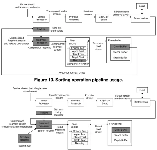
Figure 10 summarizes the pipeline usage. The data values to be sorted are stored in 2D textures. Each texture value, can have four channels; red, green, blue, and alpha (RGBA). We split the data values into the four channels. Next, we stream the data once to the GPU’s texture unit, instruct it to copy the texture into the framebuffer so that the blending operations can have access to it, and let the GPU perform the computations. When the GPU is done, we read back the data into the CPU. The GPU is able to sort the four color components in parallel. The four sorted lists are then merged back in the CPU in O(n) time. Dowd [20] proved that PBSN requireslog2n steps (lognblocks, each withlogn
phases). Since each step requires n comparisons, PBSN sorts in O(nlog2n) time. However, on the GPU, the comparisons in each phase are done in parallel. In practice, the performance is better than CPU sorting algorithms [19].
Sorting is an intermediate step in many applications. Govin-daraju et.al. made use of GPU sorting to implement an efficient JOIN operation for database and data mining computation [23]. Purcell et. al. showed how GPU sorting can be used, in con-junction with GPU search, to sort photons on a grid for Photon Mapping [21].
Figure 8. Reduction operation pipeline usage.
Figure 9. A block in the PBSN
3.4
Searching
Searchingenables us to determine if a particular element exists in a given stream. Perhaps one of the simplest forms of searching is binary search, where an element is located from a sorted list in O(logn). The element being sought is compared with the element in the middle of the sorted list. If the searched element is smaller, the search continues recursively using the left half of the list and if it is greater, using the right half of the list.
Binary search is inherently serial. To date, there is no paral-lel implementation of binary search on the GPU [4]. Thus, the focus has shifted from reducing the latency of a single search to increasing the bandwidth of the search from a given set of data. Purcell [24] showed a straightforward implementation of binary search on the GPU. The search is implemented just like it would have been on the CPU but with a fragment shader. The element being searched corresponds to a single texel in a 2D texture. So each pixel written into the framebuffer represents the result of a single search. The data set to be searched is passed into the frag-ment shader as auniformparameter, or it can simply be another texture. To really get an advantage from GPU’s binary search, one must do multiple searches using the same data set. The pipeline usage is shown in Figure 11.
3.5
Scatter and Gather
All the operations presented so far only use the back-end of the graphics pipeline (from the fragment processor on) for good
rea-sons. First, there are usually many more fragment processors than vertex processors. The GeForce 6800 has 16 fragment processors and only 6 vertex processors. Thus, we can get more parallelism using the fragment processor. Second, until recently, the vertex processor could not perform a texture fetch. Textures are impor-tant data structure for general purpose computation and without them the vertex processor’s utility is limited. Third, the fragment processor is closer to the framebuffer, where computational results are stored. Vertex processors cannot write to the framebuffer with-out going through the fragment processor.
With the GeForce 6800, things have changed a bit. The GeForce 6800 introduced texture fetch from the vertex processor, thus the vertex processor can be used to perform scatter operations. We explain how below.
Agatheroperation is anindirect-readoperation such asx=
a[i][25]. This can easily be implemented in the fragment pro-cessor by doing a texture lookup with a dependent-texture-read. A dependent-texture-read is basically a texture fetch at an offset from the current fragment’s texture coordinates.
Ascatteroperation is just the opposite of gather. It is an indirect-write of the forma[i] =x. This cannot be implemented directly using the fragment processor. The position in the framebuffer to which the fragment processor writes for each fragment is pre-determined by the rasterizer.
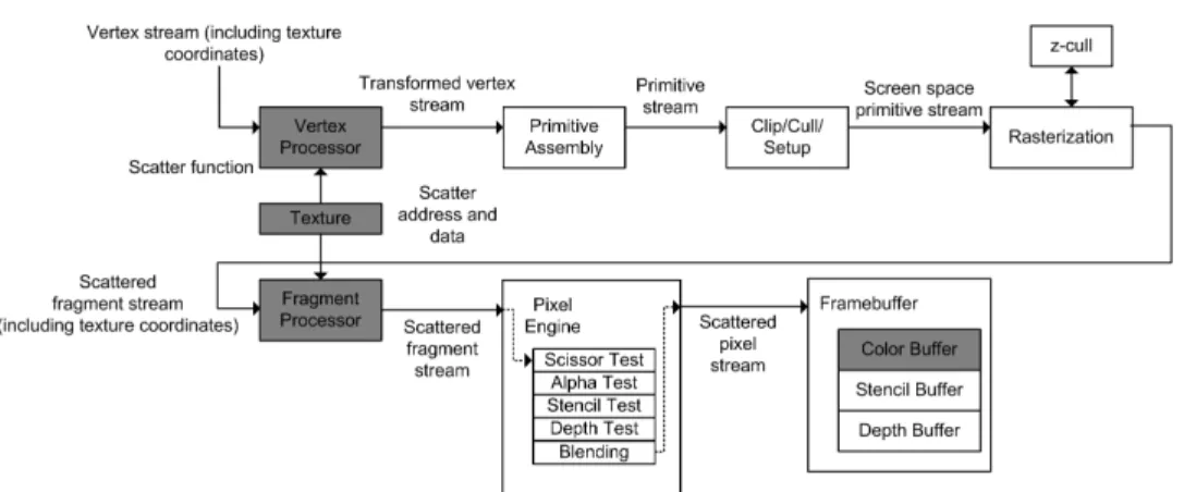
A vertex processor, however, can specify the position of ver-tices. In fact it is one of the tasks that a vertex processor is respon-sible for. So, now we can use a vertex program to perform scatter. Instead of rendering a quad, now we render a point. Previously, when a quad was rendered, the rasterizer generates fragments for every pixel covered by the quad. For a point, the rasterizer gen-erates fragments for every pixel intersecting the point. We can control the number of fragments generated by controlling the size of the point. The application simply issues points to render and the vertex processor fetches, from a texture, the scatter position and assigns it to the rendered point’s position, along with the ap-propriate data. When the fragment processor writes to the frame-buffer it will use the position specified by the vertex processor. The pipeline usage is shown in Figure 12.
3.6
Stream Filtering
Figure 10. Sorting operation pipeline usage.
Figure 11. Searching operation pipeline usage.
a stream and discard the rest. This is similar to the reduction oper-ation. The difference is that, in the reduction operation, the output size is known in advance. So we can render a quad using that size. In stream filtering, we do not have that information. The re-duction decision is now made on a per-element basis. A method calledfiltering through compaction[26] will help filter the incom-ing stream.
First choose a value to be the invalid value. The fragment pro-gram generates this invalid value to represent output that will be filtered out from the final output stream. The most straightforward way to filter the output stream is to sort the stream to eliminate invalid values. But sorting, as shown earlier, takes O(nlog2n) on the GPU. Instead, we can use a counting method called arunning sum scan(Figure 13). The running sum scan counts the number of invalid values in thecurrentelement and the (current−2i) element, whereiis theith
rendering pass, starting from 0. The re-sults are written into the framebuffer and used as input for the next pass. Afterlognrendering passes, the value at the right end of the stream indicates the total number of invalid values in the stream. This tells us the final size of the output needs to be the total length of the stream minus the value at the right end of the stream. The total running time of the sum scan is O(nlogn). There arelogn rendering passes, and each pass computes sums for a maximum of n elements.
At this point each output position knows the number of invalid values to its left, starting from its own position. Ideally we want to have a fragment program sample the valid outputs and send them into the right positions in the filtered output by shifting each valid element to the left n positions, where n is the number of invalid values to its left (as shown in Figure 14). This is basically a scatter operation. However, recall that fragment processors do not support scatter operations. We could use the vertex processor to perform the scatter (Section 3.5) but it is inefficient for large numbers of element because it does not make full use of the rasterizer.
We can, however, convert the scatter operation into a gather operation (Figure 15). One of the nice properties of therunning sum scanis that the result of the scan is a monotonically increasing sorted list. So we can use a parallel binary search to find the correct place to gather from.
Each position in the filtered output is an input for a parallel bi-nary search. The search pool is the running sum output. For each position in the filtered output, the search stops when it finds the first running sum, whose value in the original output is valid, and whose sum is equal to the distance from the element being exam-ined to the position of the running sum. For example, if we were examining the second position in the filtered output in Figure 14, the binary search would stop at the third position in the running sum output. The running sum at that value is 1 and the distance
Figure 12. Scatter operation pipeline usage.
Figure 13. Running sum scan requires logn rendering passes.
Figure 14. Stream filtering if scatter were available. Values are pushed into the filtered output.
between that running sum and the value being examined is one po-sition. It means that, in the original output, the third element has one invalid value to its left. So, we need to move it one position to the left during compaction. From Section 3.4, we see that binary search on the GPU takeslogn time for each search. So for an output of size n, the running time would be O(nlogn). But again, the searches can be done in parallel. Since running sum scan also takesnlogn, the total time is still O(nlogn).
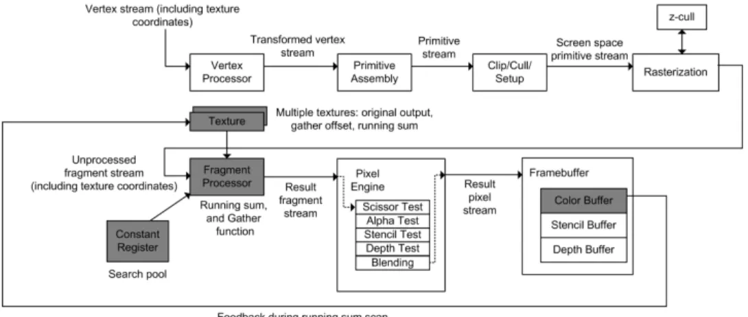
The pipeline usage for stream filtering is shown in Figure 16. Using render to texture, the original output would be a texture that is attached to the framebuffer. On top of that, we need two more textures to compute the running sum (one for input and one for putput). Once we know the size of the final output, i.e. after the running sum is done, we can render a quad of that size, perform parallel binary search, and store the results (the gather offset) in
Figure 15. Stream filtering with gather. Values are pulled from the original output.
another texture.
After that, we need one more rendering pass with a quad the size of the final output. The original output texture and the gather offset texture are both passed to a fragment program. The job of the fragment program is to fetch from the gather offset and then fetch from the original output using that offset.
3.7
Predicate Evaluation
This operation was not in Owen’s original taxonomy [4]. How-ever, people have used it, especially in database applications [27], and thus, it is a valuable addition to the taxonomy.
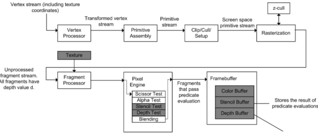
Predicate evaluationcompares each element in a stream against a constant value [27]. A single predicate evaluation can be done using thedepth test. Thedepth test comparesthe depth value of a fragment with the depth value of the corresponding pixel in the depth buffer. If the fragment passes the depth test it is written into the framebuffer, and the depth buffer at the fragment’s position is updated with the fragment’s depth value. Otherwise it is discarded. With the color buffer initialized to zero, portions of the color buffer with non-zero values are those that pass the predicate evaluation. The depth test comparison function is user specified. It includes the standardless than, andgreater thancomparators [8].
To perform the comparison, attribute values that need to be compared are stored in a 2D texture and then attached to the depth buffer portion of the framebuffer. We then render a quad with depth d, the value we want to compare the attributes against.
A series of predicate evaluations combined with the logical op-erator AND, OR, and NOT form aBoolean combination. We can use a combination ofstencilanddepthtests to perform Boolean
combinations. The stencil test compares the stencil value of a fragment’s corresponding pixel in the stencil buffer against a ref-erence value and a mask. A fragment that fails the stencil test is discarded. The comparison function is user-specified and is sim-ilar to the functions available for the depth test [8]. The stencil value in the stencil buffer can be updated based on whether the stencil test and the depth test pass or fail. There are three possible outcomes:
1. The stencil test fails.
2. The stencil test passes but the depth test fails.
3. Both the stencil and depth test pass.
A different operation can be specified for each case: 1. KEEP: keeps the current stencil value.
2. ZERO: sets the stencil value to zero.
3. REPLACE: sets the stencil value to the reference value. 4. INCR: increment the current stencil value.
5. DECR: decrement the current stencil value.
6. INVERT: bitwise inverts the current stencil value.
Each rendering pass corresponds to a predicate evaluation and after each evaluation, the stencil buffer is updated with the result of the evaluation. After the last rendering pass, non-zero values in the stencil buffer are those that pass the Boolean combination.
Figure 17 shows the pipeline usage for predicate evaluation. Notice that we do not need to use the fragment processor. Frag-ments will pass through the fragment processor unmodified. The texture unit is still shown as being used because the stencil buffer and depth buffer are actually textures that are attached to the frame-buffer.
An operation that is closely related to predicate evaluation is counting the number of attributes that pass a predicate evaluation (or Boolean combination). The GPU provides a feature called an
occlusion query. It returns the number of fragments that pass the depth test.
Database operations have also benefited from predicate evalu-ation on the GPU [27]. A basic SQL query is in the form “SE-LECT A from T where C”, where A is a list of attributes and C
is a Boolean combination of predicates. The stencil test can be used repeatedly to perform a series of predicate evaluations with the intermediate results stored in the stencil buffer.
4.
GPU Hardware Utilization Summary
As we have seen in Section 3, the GPU as a whole is capable of many operations. Figure 18 shows all the hardware used by the op-erations in Section 3. Each of the pictured GPU components have their own strengths and weaknesses within the context of general purpose computation. Clearly, one would expect that applications would use the GPU components whose strengths outweight their weaknesses. This section looks at the profile of various applica-tions to see how much different applicaapplica-tions use the programmable components of the GPU, namely the fragment processor, the ver-tex processor, and the pixel engine. Based on this analysis, the section draws conclusions about the strengths and weaknesses of each piece of hardware for GPGPU applications.
Note that one can view the GPU pipeline as having two halves, with the rasterizer as the junction between the two halves. The ras-terizer, in GPGPU applications, is used solely to interpolate ver-tices and their associated texture coordinates. While the rasterizer is used in every single operation discussed in this paper, its use is implicit so it is not highlighted in the pipeline diagrams.
4.1
Application Profiles
To quantify how much each piece of the GPU is used, several GPGPU applications were profiled. Figure 19 shows the percent-age of time each application spends in using each programmable component. These numbers are obtained from GPU hardware counters sampled using NVPerfKit [28]. Counters that track the percentage of time the fragment processor, the vertex processor, or the pixel engine was busy were sampled. Any time one of these units was not in use, the GPU could be idle, waiting for texture data, or writing to the framebuffer.
The first application is Conway’s Game of Life [29]. This ap-plication simulates a Discrete Cellular Automaton and it is mod-eled using a mapping operation which was implemented on the GPU. The second application is GPUSort [23] (described in Sec-tion 3). The third and fourth applicaSec-tions are Fast Fourier Trans-form (FFT) and Discrete Cosine TransTrans-form (DCT) as implemented on NVidia developer’s website [28]. The FFT algorithm is imple-mented as a multipass algorithm using the fragment processor. The
Figure 17. Predicate evaluation pipeline usage.
Figure 18. Summary of pipeline usage. Shaded boxes represent hardware that is used explicitly.
Figure 19. GPU hardware utilization by GPGPU applications.
DCT algorithm, the basis for JPEG compression, is also imple-mented as a fragment program. The fifth application, the Particle Engine, simulates the motion of particles as governed by the laws of physics (e.g., gravity, local forces, and collisions with primitive geometric shapes) [30].
As seen from Figure 19, applications make extensive use of the fragment processor. Furthermore, GPUSort and DCT use the pixel engine heavily. This is to be expected since we know (from Section 3.3) that the pixel engine’s blending operation is used for sorting. Note, however, that only the Particle Engine uses the vex-tex processor, other applications do not use the vervex-tex processor at all.
A key observation is that there is far greater utilization of the second half (post rasterizer) of the pipeline for GPGPU. This is an artifact of the nature of computation in the two halves. Before the rasterizer, the operations performed are per-vertex. After, they are per-fragment. Since there are many more fragments than ver-tices in a given rendering pass, GPUs have more fragment proces-sors. Thus there are more opportunities to exploit parallelism after the rasterizer. Note that maximizing the exploited parallelism in each rendering pass is of key importance in GPGPU applications because transfers of data between the GPU and CPU are expen-sive. (As an example, in the simple vector-scaling example in Sec-tion 2.2, the observed transfer rate is 1GB/sec and the observed
read back rate is 300MB/sec.) In fact, this communication is often the main bottleneck in GPGPU application performance.
4.2
Component Usage Analysis
4.2.1
Fragment Processors
The fragment processor is, by far, the most useful part of the GPU. First, there are simply many more of them than there are vertex processors. Second, they have access to the texture memory which is an important data structure for GPGPU. Their location towards the end of the pipeline also means that they can write to the framebuffer directly.
Unfortunately, the fragment processor is not able to write to random locations (scatter) in memory. The output position for each fragment is computed by the rasterizer and the fragment pro-cessor has no way of altering it. This makes some algorithms dif-ficult to implement. To overcome this limitation, one has to re-sort to either using the vertex processor (Section 3.5) to perform the scatter or convert the scatter to a gather (Section 3.6), neither of which is very appealing as they require additional rendering passes and hence degrade performance. The reason that fragment processors do not support the scatter operation is that scattering introduces write-after-read (WAR), and write-after-write (WAW) hazards. Handling these hazards adds complexity and reduces par-allelism as some fragment processors have to, for example, delay their writes until the reads of some other fragment processors com-plete. However, it could be desirable to support scatter anyway and let programmers explicitly avoid the hazards manually. This provides extra flexibility for the programmers and eliminates the additional rendering passes.
4.2.2
Vertex Processor
Like the fragment processor, the vertex processor is fully pro-grammable. However, the vertex processor has, at best, only been sparingly used for GPGPU. There are several reasons for this. First, the vertex processor is designed to operate on vertices. Since there are not as many vertices as there are fragments in single ren-dering pass, GPUs do not have as many vertex processors. As a re-sult there are fewer opportunities for parallelization. Second, ver-tex processors cannot write to the framebuffer directly since they are early in the pipeline; framebuffer writes must go through the fragment processors. Third, until recently, vertex processors did not have access to texture memory, a central GPGPU data struc-ture. The main use of the vertex processor is to make up for the short comings of the fragment processor (i.e. to perform scatter operations).
4.2.3
Pixel Engines
Pixel engines perform user-specified operations on each frag-ment and determine if that fragfrag-ment ultimately updates the frame-buffer. They are somewhat programmable. One can specify one of several functions, mostly comparison based, that are used in each rendering pass. One can also specify the action to be taken if the condition passes or fails (e.g., incrementing or decrementing the stencil value in the stencil buffer). Their use is typically limited to comparisons but they do prove useful for operations that are compare-intensive such as predicate evaluation and sorting.
5.
Conclusion
Graphics Processing Units (GPUs) are now sufficiently grammable that they could be considered a non-traditional pro-grammable processor design. Indeed, quite a number of researchers have used GPUs for general purpose applications, an area known as GPGPU. This puts GPUs in a class of designs, along with IBM’s Cell processor among others, that are of great interest to processor designers. In this paper, we show that by studying how GPU hard-ware is used by GPGPU applications, one can gain insight in how to design non-traditional parallel machines.
In order to understand how application developers are using GPU hardware, we examined how each operation in Owen’s tax-onomy [4] utilized the underlying hardware. Since this taxtax-onomy of GPGPU operations (augmented with the predicate-evaluation operation) covers the space of currently known GPGPU applica-tions, this examination clearly illustrates the portions of the GPU pipeline that are sufficiently “general-purpose”.
Of the two halves of the GPU pipeline (the first half consists of the stages before the rasterizer, the second half the stages after), we find that the second half of the pipeline is most suited to general purpose computation. One reason for this is that there are simply more fragments than there are vertices in graphics applications, and thus GPUs are designed with more hardware resources in the second half of the pipeline. More hardware resources leads to more opportunities for exploiting parallelism, and amortizing the costs of transporting data to and from the main CPU. We found that another reason for the bias toward the second half of the pipeline is that, until recently, only the fragment processors had sufficient ac-cess to a general-purpose-like memory (the framebuffers and tex-ture memory). In fact, the vertex processor is the only hardware in the first half of the pipeline that is explicitly used for GPGPU. Its sole purpose is to perform scatter operations that the fragment pro-cessor cannot perform. If the fragment propro-cessor were enhanced to support scattering, the vertex processor would be useless in ex-isting GPGPU applications. Given these observations, we believe that (1) supporting scatter (with limited hazard detection) in the fragment processor is worthwhile, and (2) that it is worth explor-ing processor designs that resemble the second half of the GPU pipeline as an alternative (or addition) to traditional Von-Neumann machines.
6.
References
[1] M. Ekman, F. Wang, and J. Nilsson, “An in-depth look at computer performance growth,”SIGARCH Comput. Archit. News, vol. 33, pp. 144–147, March 2005.
[2] P. Trancoso and M. Charalambous, “Exploring graphics processor performance for general purpose applications,” in
8th Euromicro Conference on Digital System Design (DSD), pp. 306–313, 2005.
[3] E. Lindholm, M. Kilgard, and H. Moreton, “A
user-programmable vertex engine,” inProceedings of ACM SIGGRAPH, Computer Graphics Proceedings, Annual Conference Series, pp. 149–158, 2001.
[4] J. Owens, D. Luebke, N. Govindaraju, M. Harris, J. Kr¨uger, A. Lefohn, and T. Purcell, “A survey of general-purpose computation on graphics hardware,” inEurographics 2005, State of the Art Reports, pp. 21–51, August 2005.
[5] J. Owens, “Streaming architectures and technology trends,”
GPU Gems 2, pp. 457–470, March 2005.
[6] I. Buck, T. Foley, D. Horn, J. Sugerman, K. Fatahalian, M. Houston, and P. Hanrahan, “Brook for gpus: Stream
computing on graphics hardware,”ACM Transactions on Graphics (TOG), vol. 23, pp. 777–786, 2004.
[7] M. Flynn, “Some computer organizations and their effectiveness,”IEEE Transactions on Computers, vol. C-21, pp. 948–960, September 1972.
[8] M. Segal and K. Akeley, “The opengl graphics system: A specification, version 2.”
http://www.opengl.org/documentation/specs/, October 2004. [9] E. Kilgariff and R. Fernando, “The GeForce 6 series GPU
architecture,”GPU Gems 2, pp. 471–491, March 2005. [10] “Microsoft’s directx sdk.”
http://msdn.microsoft.com/directx/sdk/readmepage/default.aspx, February 2006.
[11] J. Kessenich, D. Baldwin, and R. Rost, “The opengl shading language, version 1.10, rev. 59.”
http://www.opengl.org/documentation/specs/, October 2004. [12] E. Kilgariff and R. Fernando,The Cg Tutorial: The
definitive Guide to Programmable Real-Time graphics. Addison-Wesley, 2003.
[13] C. Thompson, S. Hahn, and M. Oskin, “A framework and analysis of modern graphics architectures for
general-purpose computing,” inProceedings of the 35th Annual International Symposium on Microarchitecture, pp. 215–226, November 2002.
[14] D. Tardity, S. Puri, and J. Oglesby, “Accelerator: simplified programming of graphics processing units for
general-purpose uses via data parallelism,” MSR-TR-2005-184, Microsoft, 2005.
[15] M. Harris, G. Coombe, T. Scheuermann, and A. Lastra, “Physically-based visual simulation on graphics hardware,” inProc. 2002 SIGGRAPH / Eurographics Workshop on Graphics Hardware, pp. 1–10, 2002.
[16] A. LaMarca and R. Ladner, “The influence of caches on the performance of sorting,” inProceedings of the Eighth Annual ACM-SIAM Symposium on Discrete Algorithms, pp. 370–379, 1997.
[17] J. Zhou and K. Ross, “Implementing database operations using SIMD instructions,” inProceedings of the ACM SIGMOD International Conference on Management of Data, pp. 145–156, June 2002.
[18] D. Knuth,The Art of Computer Programming Volume 3. Addison-Wesley, 1973.
[19] N. Govindaraju, N. Raghuvanshi, and D. Manocha, “Fast and approximate stream mining of quantiles and frequencies using graphics processors,” inProceedings of the ACM SIGMOD International Conference on Management of Data, pp. 611–622, 2005.
[20] M. Dowd, Y. Perl, L. Rudolph, and M. Saks, “The periodic balanced sorting network,”Journal of the ACM (JACM), vol. 36, no. 4, pp. 738–757, 1989.
[21] T. Purcell, C. Donner, M. Cammarano, H. Jensen, and P. Hanrahan, “Photon mapping on programmable graphics hardware,” inProceedings of the ACM
SIGGRAPH/EUROGRAPHICS conference on Graphics hardware, pp. 41–50, July 2003.
[22] P. Kipfer, M. Segal, and R. Westermann, “Uberflow: A GPU-based particle engine,” inProceedings of the ACM SIGGRAPH/EUROGRAPHICS conference on Graphics hardware, pp. 115–122, August 2004.
[23] N. Govindaraju, N. Raghuvanshi, M. Henson, D. Tuft, and D. Manocha, “A cache-efficient sorting algorithm for database and data mining computations using graphics processors,” Tech. Rep. TR05-016, University of North Carolina, 2005.
[24] T. Purcell, I. Buck, and P. Hanrahan, “Ray tracing on programmable graphics hardware,”ACM Transactions on Graphics (TOG), vol. 21.
[25] I. Buck, “Taking the plunge into GPU computing,”GPU Gems 2, pp. 509–519, March 2005.
[26] D. Horn, “Stream reduction operations for GPGPU applications,”GPU Gems 2, pp. 573–589, March 2005. [27] N. Govindaraju, B. Lloyd, W. Wang, M. Lin, and
D. Manocha, “Fast computation of database operations using graphics processors,” inProceedings of the ACM SIGMOD International Conference on Management of Data, pp. 215–226, June 2004.
[28] “developer.nvidia.com.”
http://developer.nvidia.com/page/home.html. [29] M. Gardner, “Mathematical Games, The fantastic
combinations of John Conway’s new solitaire game of life,”
Scientific American 223, pp. 120–123, October 1970. [30] L. Latta, “Building a million particle system,”Game