Reviving Beta? Another look at the cross-section of average share returns on the JSE

(1)

Reviving Beta?

Another look at the cross-section of average share returns on the JSE

(2)

A 50% dissertation to be submitted in partial fulfilment for the degree of: MASTERS OF COMMERCE (FINANCE)

UNIVERSITY OF THE WITWATERSRAND

NAME OF STUDENT: Daniel Page

NAME OF SUPERVISOR: Christo Auret

DATE: 29 February 2012

Declaration

I hereby declare that this is my own unaided work, the substance of or any part of which has not been submitted in the past or will be submitted in the future for a degree in to any university and that the information contained herein has not been obtained during my employment or working under the aegis of, any other person or organization other than this university

Name of Candidate Signed

...

(3)

ABSTRACT

Van Rensburg and Robertson (2003a) stated that the CAPM beta has little or no relationship with returns generated by size and price to earnings sorted portfolios. This study intends to demonstrate that a reformulated CAPM beta, estimated using return on equity as opposed to share returns, unravels the size and value premium. The study proves that the “cash-flow” generated beta partially explains the cross-sectional variation in share returns when measured over the long run, specifically when portfolios are sorted on book to market, however the cash flow beta is less successful when attempting to explain the small size premium. The premise of the study is that the cash flow dynamics of share returns eventually dominate the first and second moments and thus result in cash flow based measures of risk and return that should succeed in explaining the cross-sectional variation in share returns. The study makes use of vector autoregressive models in order to examine the short term effect of structural shocks to the cash flow fundamentals of a stock or portfolio through impulse response functions as well as quantifying a long-term relationship between cash flow fundamentals and share returns using a VECM specification. The study further uses fixed effects, random effects and GMM/dynamic panel data cross-sectional regressions in order to examine the ability of the cash flow beta explaining the value and size premium. The results of the study are mixed. The cash flow beta does well in explaining the returns of portfolios sorted on book to market, but fails to do the same with size sorted portfolios. In the cash flow betas favour, it performs far better than the conventionally measured CAPM beta throughout the study.

(4)

Definition of Terms

CAPM: The capital asset pricing model of Sharpe (1964), Lintner (1965) and later Black (1972). The model states that under rational and homogenous expectations with regards to risk and return, the market risk of an asset, proxied by the market beta is the sole determinant of an assets expected return.

Cash flow beta: The cash flow beta per Cohen, Polk and Voulteenaho (2008) where beta is estimated using cash flow fundamentals of the underlying asset in question

ROE: The return on equity of a share is considered by Cohen, Polk and Voulteenaho (2008) as the monthly change in book value per share (inclusive of gross dividend payments)

VAR: Vector autoregressive models are multivariate time-series models that utilise both lagged independent as well as dependent variables in explaining time-series data

IRF: Impulse response functions utilise the estimated VAR’s as a system and allow one to study the interaction between variables within a VAR. This involves tracing the marginal effect of a shock in one variable and its effect on another

Variance Decompositions: Otherwise known as the forecast error variance decomposition – Allows one to decompose the variation in a forecasted variable due to a shock in another variable

VECM: Vector Error Correction Model allows for the estimation of long term relationships in non-stationary data based on cointegration between the variables in a VAR

I(1): A non-stationary variable is said to be integrated of order one if it is stationary after being differenced once, this implies that if a variable is I(n), it is only stationary after being differenced n times

Cointegration: Variables are said to be cointegrated of order one if a combination of the non-stationary variables yields a stationary time series

LR test: A statistical test that determines whether a VECM restriction is binding

B/M: Book to market is the book value of a share scaled by the market price of the share. The book to market ratio is the inverse of the popularised price to book ratio

(5)

Figure 1 Book to Market sorted portfolios (No restriction and 50 cent restriction) 16 Figure 2 Size sorted portfolios (No restriction and 50 cent restriction) 17 Figure 3 Impulse Response Function – 5 year value sort (50 cent restriction) 20 Figure 4 Impulse Response Function – 5 year size sort (50 cent restriction) 21 Figure 5 Variance Decomposition – 5 year value sort (50 cent restriction) 22 Figure 6 Variance Decomposition – 5 year size sort (50 cent restriction) 23

Figure 7a Cash flow beta – Value Sort 33

Figure 7b Cash flow betas – Size Sort 34

Figure 8 Cash flow betas – Size and Value sort (7 year holding period) 35

Figure 9a Cash flow betas – Value Sort (50 cent restriction) 40

Figure 9b Cash flow betas – Size Sort (50 cent restriction) 41

Figure 10a Cash flow betas – Value Sort (Equally weighted market ROE) 45

(6)

Table of Tables

Table 1a VECM output for level ROE, JSE and Value Portfolio (50c Restriction) 25

Table 1b VECM output for the level ROE, JSE and value portfolio with restriction β12=β13 26

Table 2 VECM output for the level ROE, JSE and small size portfolio 27

Table 3a VECM output for the level ROE, JSE and HML level portfolio 28

Table 3b VECM Restriction results using SMB and HML as dependent variables 28

Table 4a Sample Statistics – Value Sort 31

Table 4b Sample Statistics – Size Sort 32

Table 5a GMM and Fixed effects regression results – Value Sort 36

Table 5b GMM and Fixed effects regression results – Size Sort 37

Table 6 GMM and Fixed effects regression results – Size and Value Sort 38

Table 7a GMM and Fixed effects regression results – Value Sort (50c price filter) 42

Table 7b GMM and Fixed effects regression results – Size Sort (50c price filter) 44

Table 8a GMM, Fixed and Random effects regression results – Value Sort (Equally – weighted market proxies)

46

Table 8b GMM, Fixed and Random effects regression results – Size Sort (Equally – weighted market proxies)

(7)

A. Introduction

The CAPM in its current form presents a logical conundrum. Markowitz (1959) stated that the risk of an asset should be the sole determinant of expected return. The theory was further extended by Sharpe (1964), Lintner (1965) and Black (1972) to consider the effects of diversification and the result was a two-parameter model that consisted of a risk-free or zero beta asset and an ex-ante efficient market portfolio. Their combined findings led to the capital asset pricing model, where risk (and therefore expected return) is explained by a single factor, the CAPM beta, which is the covariance of an assets return to that of the market portfolio, scaled by the variance of the market portfolios return. The fields of financial economics, investment and corporate finance are plagued with inconsistency as one is introduced to the theory of CAPM and the concept of market efficiency as if they are gospel, yet the natural progression of a financial economist is to learn that the CAPM and market efficiency only hold in theory, and that in the ‘real world’ CAPM fails in explaining the cross-sectional variation in historical share returns and therefore, the model is relegated to the annals of theoretical history. There have been a number of attempts to salvage the CAPM by making modifications (varying from slight to extreme) both to the theory as well as the composition of the asset pricing model, yet the general consensus holds that CAPM in its original form is void, albeit theoretically appealing. The purpose of this study is to consider and test a variation of the CAPM and identify whether the modified CAPM has the ability to succeed where others have failed.

The methodology of Cohen, Polk and Vuolteenaho (2008) is employed in order to derive a “cash-flow” beta, where beta is estimated using cash flow returns proxied by monthly changes in book equity (referred to as return on equity or ROE), as opposed to dividend adjusted share returns. The central hypothesis of the study is to identify whether the cash flow beta is more successful than the conventional CAPM beta in explaining the cross-sectional variation in returns of shares listed on the Johannesburg Stock Exchange (“JSE”). The study employs an assortment of econometric methodologies in order to determine the effectiveness of the proposed cash flow beta and offer additional robustness. A number of sub-hypotheses are presented that extend to the central hypothesis of the study.

The sample period of the study is from January 1995 to June 2009 (fourteen and a half years) and includes all shares listed on the JSE over the period. As with most studies of this nature,

(8)

data are sorted into portfolios based on independent size and value criteria, where value is proxied by the book value per share scaled by the market value per share (book to market ratio) and size by the natural logarithm of market capitalisation of the share in question. The study is split into two sub-studies where the first employs time-series based econometric tests while the second, cross-sectional regressions. All the methodologies employed find that there is both an persistent size effect and value premium present on the JSE, in line with the findings of Van Rensburg and Robertson (2003a), Graham and Uliana (2000), Basiewicz and Auret (2009) and Strugnell, Gilbert and Kruger (2011).

In the time-series experiments, VAR’s are estimated and impulse response functions as well as variance decompositions are conducted in order to decompose the effect of different factors on the value and size sorted portfolio returns. The results indicate that the ROE of the extreme size and value portfolios contribute minimally to monthly return and the variation in return of the extreme value and small cap portfolio. The tests also include the ROE market proxy as well as the JSE All share index. The results of the impulse response functions are mixed. The value portfolio seems to be very sensitive to a shock to the overall cash flow return of the market, while the small size portfolio is more sensitive to a shock to the JSE. The variance decompositions indicate that a shock to the ROE of the market seems to contribute more to the variation in the size and value portfolio returns. A VECM is then estimated in order to compare the long-run relationships between the different portfolios and the JSE as well as the ROE market proxy. The findings indicate that the extreme value and small size portfolios have positive long run relationships with the ROE market proxy, strengthening the notion that the size and value effect is affected by the overall cash flow return of the market, contributing to the case for the cash flow beta. However, when estimating VECM’s based on the excess returns earned by the high minus low and small minus big trading strategies, the ROE market proxy fails to maintain a significant long run relationship with the level excess returns.

The second part of the study focuses on the cross-sectional properties of the different portfolios sorted on value and size. Portfolios are sorted yearly and are held for 60 months post sort. Initially, value and size sorts are conducted separately where nine portfolios are constructed on book to market and ten on size. The second sort is a simultaneous size and value sort consistent with the methodology employed by Basiewicz and Auret (2009). Cohen,

(9)

Polk and Voulteenaho (2008) considered estimating a cash flow beta based on accounting data and employed an arithmetic book value return referred to as return on equity (“ROE”). The ROE of a share is defined as the natural logarithm of a shares arithmetic book value holding period return, while the ROE of the market is the natural logarithm of the arithmetic book value holding period return of the value weighted market portfolio. Using a similar procedure to that employed by Cohen, Polk and Vuolteenaho (2008), cash flow betas are calculated over different holding periods for each of the portfolios and estimated using rolling window OLS regressions. The purpose of the exercise is to identify the evolution of the cash flow beta over time.

The findings are similar to that of Cohen, Polk and Vuolteenaho (2008) as the cash flow betas of the value portfolios are initially low, yet increase monotonically over time and eventually overtake the cash flow betas of the growth portfolios. The same phenomenon is not apparent for the portfolios sorted on size as the small size portfolios cash flow betas fail to increase over time and do not surpass the cash flow betas of the large capitalization portfolios. In this study, regressions are run using both fixed effects and GMM regressions and the results are once again consistent with the findings of Van Rensburg and Robertson (2003a), as there is both a significant value and size premium when shares are simultaneously sorted on size and value criteria1. The initial cross-sectional tests indicate that the conventionally measured CAPM beta fails to explain the cross-sectional variation in share returns and is consistently negative and significant. The cash flow betas performance is mixed as it succeeds in explaining the cross-sectional variation in the returns of portfolios sorted on value, but not on size. In the simultaneous value and size sort, the cash flow beta is significant when using the GMM specification, while the fixed effects regression finds the cash flow beta to be significant, but only at the 10% level. The success of the cash flow beta explaining the value premium may be attributed to the cash flow beta being a construct of the book to market ratio. A further interesting finding is that throughout the univariate and multivariate regressions, the CAPM beta produces a consistently negative coefficient, in line with the recent findings of Strugnell, Gilbert and Kruger (2011). In order to comprehensively test the cash flow beta, a price filter is applied in order to determine whether the failure of the cash flow beta in explaining the size premium is attributable to illiquidity. The results indicate that

1

(10)

illiquidity is not the cause of the cash flow betas poor performance. Cash flow and CAPM betas are also estimated using equally-weighted market proxies in order to test whether the cash flow betas failure is attributable to concentration found in the JSE ALSI and the ROE market proxy. The results indicate that the failure of the cash flow beta in explaining the small size premium is not attributable to the concentration or inefficiency of the market proxy.

B. Literature Review

a) International Literature

Two popular phenomena in asset pricing theory that have received much attention are the small size effect and the value premium. The size effect can be summarized as the excess return earned by low capitalization stocks over large capitalization stocks. Banz (1981) was credited with the identification of the size effect or small firm premium and found that the presence of the size effect is persistent and fails to reconcile with CAPM as large capitalization shares tend to have larger betas yet achieve lower average returns than small capitalization shares. Reinganum (1981) concluded that the presence of an unquestionable and consistent size effect is in direct contravention with the theory of efficient markets and the CAPM.

The value effect entails that firms with a higher ratio of accounting based share value or earnings scaled by the firms market price per share tend to outperform shares at the other end of the spectrum, aptly named ‘growth’ shares due to their relatively high market value. Basu (1983) found that the earnings-to-price (“E/P”) ratio helped to explain the cross-sectional variation in share returns. Rosenberg, Reid and Lanstein (1985) found that the book-to-market ratio (“B/M”) has a significantly positive relationship with the average return. Chan, Hamao and Lakonishok (1991) found that B/M is a significant variable when attempting to explain the cross-sectional variation in returns of Japanese stocks.

A number of other less popular anomalies that have received international attention are the ‘leverage effect’ of Bhandari (1988), where leverage was found to have a positive relationship with average returns. Rozeff and Kinney (1976) found that the risk-adjusted returns of shares in January where significantly higher than returns achieved in any other

(11)

calendar month. Debondt and Thaler (1985) found that past long-term losers consistently outperformed past long-term winners, while Jegadeesh and Titman (1993) found that past short-term winners outperformed past short-term losers, otherwise known as the “momentum” effect.

Fama and French (1992) conducted a comprehensive study and tested a number of conventionally used value and size proxies in order to isolate which was the most accurate and to determine whether size and value possess independent explanatory power on a cross-section of US listed stocks. The authors found that size (proxied by the natural log of market capitalization) and value (proxied by B/M) where both significantly powerful when explaining the cross-sectional variation in share returns. Fama and French (1993) concluded that risk is multidimensional and developed a pricing model that incorporates variables that represent both the value and size premium independently. The proposed model proved powerful in explaining the cross-sectional variation in share returns yet lacked a meaningful theoretical motivation for incorporating additional factors within a pricing model. Fama and French (1995) hypothesized that both the size and value premium are related to profitability, therefore the conventional CAPM beta fails to capture information regarding earnings potential and profitability. The authors acknowledged that their findings leave a number of central issue unanswered, namely; why does the CAPM beta, which in theory should be the sole determinant of risk and therefore return, fail to explain the variation in return.

Roll (1977) held that the CAPM in its current form cannot be tested and that any attempt to disprove or even test the validity of the CAPM would result in a type 1 or type 2 error, ie accepting the CAPM when it is false or rejecting the CAPM when it is true. In lieu of such opinion, the CAPM actually stood as untestable and in some sense unusable. Ross (1976) and later Chen, Roll and Ross (1986) developed arbitrage pricing theory (“APT”), where based on the lack of usability or testability of the CAPM, an asset pricing model was developed that utilises a number of macroeconomic factors that are tested to find a contemporaneous relationship with returns .On the basis of significant contemporaneous relationships, macroeconomic factors are incorporated into a pricing model. The APT, much like the Fama-French three factor model, lacks the theoretical foundation of the CAPM, yet succeeds in explaining a larger portion of the cross-sectional variation in share returns. The model of Fama and French (1993) is not dissimilar to the APT, as the model utilises variables that aid

(12)

in the explanation of the cross-sectional variability in returns yet are solely based on consistent empirical relationships.

A fundamental problem when considering both the size and value premium is that their presence on an international scale is actually a joint rejection of the CAPM and the efficient market hypothesis. Without a meaningful explanation of the risks inherent in high value or small size firms, one is left to conclude that such anomalies are a rejection of market efficiency. If risks are not priced, then the market should not reward an investment or an asset with a higher return. In light of this, a number of financial economists endeavoured to explain the size and value premiums in order to salvage both the CAPM and the theory of efficient markets.

A stream of literature has emerged that considers cash flow fundamentals as a key in explaining the variation in share returns. Da (2009) builds on the consumption based CAPM or CCAPM of Rubinstein (1976), Lucas (1978), and Breeden (1979) and successfully decomposes share returns into a cash flow duration and cash flow covariance with aggregate consumption. The author found that the variation in share returns over long periods can be directly linked to fundamental cash flow fundamentals. Nekrasof and Shroff (2006) found that that a single-factor risk measure, based on the accounting beta estimated from cash flow fundamentals (accounting data) was able to largely explain the “mispricing” in value and growth stocks.

Campbell and Vuolteenaho (2004a) propose a version of Merton’s (1973) Intertemporal Capital Asset Pricing Model (ICAPM), in which investors care more about permanent cash-flow-driven movements than about temporary discount-rate-driven movements in the aggregate stock market. The theory relies on the logic that cash flow innovations should have a greater and more permanent effect on share returns as investors will naturally be more concerned with a cash flow change to an investment than a discount rate change. Considering a simple dividend paying asset, a negative shock to the cash flow component would result in a decrease in the present value, as would an increase to the discount rate, yet an increase to the discount rate would be compensated in the long run with a higher return. The authors decomposed beta into a ‘good’ and ‘bad’ beta, where the bad beta relates to a shares cash

(13)

flow beta. The authors found that including both betas within in an asset pricing framework, greatly improved the performance of the standard CAPM.

Campbell (1991) and Campbell and Ammer (1993) use the dividend growth model proposed by Campbell and Shiller (1998a) to decompose share returns into news about cash flows and discount rates using vector auto-regressions (VAR). The process involves modelling discount rate news and backing out the cash flow related news as a residual. Voulteenaho (2000) developed a present value model that utilised ROE instead of dividend growth. Voulteenaho (2002) utilised the ROE based model and a VAR variance decomposition in order to determine the relative effect of cash flow innovations on the variation in share returns. The author found that firm level share returns are predominantly driven by cash flow fundamentals. A further finding was that a positive shock to the cash flow or good news attributable to cash flow is followed by a positive shock to return.

Campbell, Polk and Voulteenaho (2009) employed a similar methodology to that of Campbell (1991) and estimated a VAR in order to decompose firm-level stock returns of value and growth stocks into components driven by cash-flow shocks and discount-rate shocks. The authors found that both the variation in growth and value stocks is explained by the cash flow components derived from the VAR model. The authors further employed a cash flow based measure of ROE and regressed the ROE’s of growth and value shares on the two components of the market return estimated by Campbell and Vuolteenaho (2003). The authors found that value stocks’ ROE is more sensitive to market’s cash-flow news than that of growth stocks and that growth stocks’ ROE is more sensitive to the market’s discount-rate news than that of value stocks.

Chen and Zhoa (2009) considered the methodology prescribed by Campbell and Shiller (1988a) and Campbell (1991) and found that the method of estimating discount rate news using VAR and backing out cash flow news as a residual carries a significant amount of imprecision. The authors noted that from a theoretical standpoint, the methodology would work, if and only if the model used perfectly replicated the data generating process of returns, which is never the case. The authors found that when attempting to replicate the results of Campbell, Polk and Voulteenaho (2009), they found that value shares did not have

(14)

significantly higher cash flow betas nor did growth shares have significantly higher discount rate betas.

Cohen, Polk and Voulteenaho (2008) found that using the cash flow based measure of profitability (ROE) proposed by Voulteenaho (2000) in order to estimate beta, resulted in a cash flow beta estimation that monotonically increases for high value shares and decreases for growth shares. The authors noted that previous joint tests of market efficiency and CAPM lack power as they employ the estimation of profits/returns earned from dynamic trading strategies and reject the joint hypothesis based on economically high Sharpe ratios. The authors hypothesized that a buy-and-hold methodology of estimating portfolio returns was more theoretically appealing as it allowed for the examination of the long run behaviour of share returns. Convention dictates that a rational investor would not act like a trader and engage in extreme trading strategies that could potentially result in extreme losses and significant trading costs. Long-term investors or mutual funds are generally constrained from participating in extreme trading; therefore the authors employed a methodology that they considered a more accurate real-time test of the CAPM as it would mimic the possible actions of a conventional buy-and-hold investor.

The authors hypothesized that the cash flow fundamentals of an asset begin to dominate the first and second moments of returns in the long run, therefore the imprecision of the conventionally estimated CAPM beta is due to the inherent noise that plagues high frequency share returns. The authors conjectured that by estimating long run cash flow beta’s using the discounted ROE of a share and the discounted ROE of the market, one would derive a beta estimation that succeeds in explaining the value premium. The authors found that consistent with the results of Fama and French (1992, 1993,1996) and Lakonishok, Shleifer, and Vishny (1994), growth stocks have higher CAPM betas than value stocks.

The authors proposed a methodology of constructing portfolios yearly based on a price-to-book sort and holding the portfolios for 15 years post sort. The authors then calculated the persistence of the price to book value within portfolios and also estimated the evolution of conventional CAPM betas and cash flow betas over time. The authors found that within five years post sort, on average the cash flow betas of the value portfolios increased significantly

(15)

and were higher than the cash flow betas of the growth portfolios. The authors confirmed their findings by running cross-sectional regressions and found that the estimated cash flow beta succeeded in explaining the cross-sectional variation in share returns.

The thematic similarity between the above paper and that of Campbell and Shiller (1988a) is that the cash flow fundamentals play a significantly larger role in the determination of risk premia. The general theme of the study implies that the joint hypothesis of market efficiency and the CAPM hold approximately in the long-run. This implies that the excess return earned on high minus low value or small minus big investment strategies can be successfully explained by cash-flow risk and the risk inherent in such strategies is priced (eventually). The findings emphasize the notion that the cash-flow based methodology of estimating beta delivers a ‘good’ approximation of price level returns. The implications of such findings are that a slight methodological change to the CAPM may be able to rationalize the conflict between investment and corporate finance as areas of study and reconcile the usage of CAPM in capital budgeting and valuation. Furthermore, the findings imply that markets are actually efficient in the long-run as cash-flow risks are priced into the excess returns of value and small cap shares.

b) South African Literature

The evidence of both the size and value premia in South African literature is mixed. De Villiers, Pettit and Affleck-Graves (1986), Bradfield, Barr and Affleck-Graves (1988), Page and Palmer (1993) and more recently Auret and Cline (2011) found no significant size effect on the JSE. Page (1996),Van Rensburg (2001),Van Rensburg and Robertson (2003a), Auret and Sinclaire (2006), Basiewicz and Auret (2009) and Strugnell, Gilbert and Kruger (2011) found both a significant size and value effect on the JSE. Notably, Van Rensburg and Robertson (2003a) stated that previous studies that failed to detect the small size effect were biased due to the small sample sizes and time frames employed.

Van Rensburg and Robertson (2003a) concluded their study with the statement that their findings were an unambiguous contradiction of the CAPM as they found that CAPM beta had a negative relationship with average returns over the sample period. Strugnell, Gilbert and

(16)

Kruger (2011) considered the results of Van Rensburg and Robertson (2003a) and conducted a similar study over a longer time frame and similarly concluded that there is both a significant size and value effect found on the cross-section of share returns on the JSE. More importantly, the authors found that beta “is irrelevant as far as return generation on the JSE is concerned, at least based on the possibly inefficient market proxy of the FTSE-JSE All – Share Index. Basiewicz and Auret (2009) conducted a similar study to Fama and French (1992) and found that there is both a significant and independent value and size effect on the JSE and that B/M is the best proxy for value, in line with the findings of Auret and Sinclaire (2006).

Van Rensburg and Robertson (2003a) considered the variation in share returns when sorting portfolios based on size, price-to-earnings (P/E) and pre-ranking beta. The authors conducted a two way sort where stocks were sorted (monthly) initially based on size and then on P/E. Basiewicz and Auret (2009) considered the findings and the methodology of Van Rensburg and Robertson (2003a) and conducted a study where portfolios were sorted yearly as opposed to monthly and the size and value sort was conducted simultaneously in order to allow for independent variation based on size and value. The authors found both a significant size and value effect and that B/M was the best proxy for value. These findings were consistent, if not less extreme, than Auret and Sinclaire (2006) as the latter found that B/M, when included in multivariate regressions, subsumed the size effect.

Basiewicz and Auret (2009) conducted an intensive study that considered the effects of a number of methodological variations as well as practical constraints applied to a typical investor. The study considered the effects of transaction costs, liquidity constraints and returns calculated using both equally and value weighted portfolios. The authors found that the application of price and liquidity restrictions resulted in dampening on the size and value premium. The authors also found that equally-weighted portfolio returns generally exceeded value-weighted returns.

Strugnell, Gilbert and Kruger (2011) questioned whether the findings of Van Rensburg and Robertson (2003a) where sample specific and whether the conventional method of estimating the CAPM beta using ordinary least squares contributed to the poor performance of the

(17)

CAPM beta in explaining the cross-sectional variation in share returns on the JSE. Cloete, De Jongh and De Wet (2002) found that by combining the estimation techniques developed by Vasicek (1973) and Williams (1977) resulted in estimations of beta that performed better when compared to other beta estimation methodologies. Strugnell, Gilbert and Kruger (2011) considered a larger sample period and utilised a number of methodologies when estimating beta in order to correct for thin trading. Betas were estimated using at least 60 months of historical return as described by Bradfield (2003). In line with the findings of Cloete, De Jongh and De Wet (2002), the authors hypothesized that the negative relationship found between beta and average returns in Van Rensburg and Robertson (2003a) may have been partially due to methodological bias in estimating beta.

The size and value effect as well as the testing of the joint-hypothesis of the CAPM and market efficiency have received much attention in South African literature; however the usage of accounting based return measures in order to explain the return data generating process as well as the cross-sectional variation in returns has received little attention. Taylor (1995) considered the potential lack of precision in estimating accounting based return, specifically accounting rate of return, return on assets, return on equity and earnings yield and proposed that accounting measures of return contain important informational content despite the inherent bias and potential estimation error related to accounting data.

Bergesen and Ward (1996) conducted a thorough study on the descriptive power of financial ratios and their relationship with beta. The authors found that beta possessed a positive relationship with firm growth, profitability and size. The authors further found that the cash flow and profitability measures used where significant throughout the study yet, the estimated cash flow beta was insignificant throughout the study. The findings of the authors seem to be consistent with later literature as the results imply a size and value effect. The study differs methodologically to later studies as the authors tested the significance of accounting based ratios in relation to beta as opposed to actual returns. The finding of beta possessing a positive relationship with size and profitability implies that both growth and large cap firms should have higher CAPM betas. Furthermore, the accounting measures used to proxy cash flow and profitability seemed to possess a positive relationship with returns over the period of study

(18)

C. Data

The time period of the study conducted is January 1995 to June 2009 and the Findata@Wits database was the sole data source used. All shares listed on the Johannesburg Stock Exchange (“JSE”) over the time period were considered. Findata@Wits database utilises a number of data and information sources. I-Net Bridge and McGregor BFA were the main sources of price, dividend and accounting data. In order to account for corporate actions, JSE monthly bulletins were used. Shares that exit the sample due to delisting or suspension are given a zero return and are deemed not listed in order to account for potential survivorship bias. The FTSE-JSE ALSI (“JSE”) is used as the market proxy, consistent with similar studies conducted on the JSE.

The results are split into two separate sets of tests that utilise differing methodologies. In order to accommodate the time-series properties of the data, time-series econometric tests are employed in order to determine whether the proposed cash-flow beta and its construction are viable when employing a time-series based approach. The second set of tests relies on the panel properties of the data. Cross-sectional regressions are run using fixed effects and GMM/dynamic panel regressions in order to correct for the potential estimation bias that can occur when data has both cross-sectional and time-series properties. The utilization of two different regression procedures allows for comparisons to be drawn between the estimations, while consistent results across specifications adds further robustness to the study. As mentioned previously, the central hypothesis of the study is to determine whether a modified methodology of estimating beta results in a measure that successfully describes the cross-sectional variation in average returns on the JSE.

D. Time-Series Tests

a) Preliminary Tests

Data is initially sorted according to size and value separately, where size is proxied by the natural log of market capitalization and value by the book-value per share scaled by the market-value per share. Shares are sorted into one of three portfolios based on their previous year’s median book to market or average size. Portfolio break points, based on the lower 33rd and upper 66th percentile, are inserted at each sorting point and stocks are categorised

(19)

accordingly. The average equally weighted returns a

three long-term strategies where holding periods are three, five and seven years construction is intended to mimic medium

long term (seven year) buy-and-hold investment strategy.

Various holding periods are used in order to simulate the methodology of

Voulteenaho (2008). Holding portfolio constituents constant over longer holding periods affords one the ability to identify whe

The usage of three portfolios also allows for

portfolios and should allow for each portfolio to contain a larger number of shares of each holding period. Basiewicz and Auret (2009) utilise

determine the effect of liquidity and transaction costs on the size and value premium. A price filter of 100, 75 and 50 cents is applied to the portfolio in order to ascerta

of the extreme portfolios. To make the study tractable, the results of the five year sorts 50 cent price filter are presented (See Appendix 1)

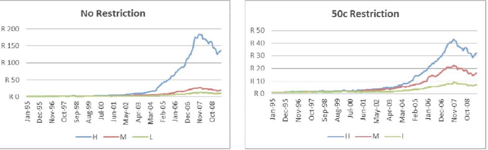
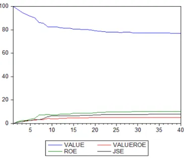
Figure 1: Value sorted portfolios restriction)

Figure 1 indicates that there is a significant value effect when sorting portfolios based on median B/M and holding portfolios for five years post sort. Such findings are consisten the findings of Van Rensburg and Robertson (20

2

This implies that the medium term investment results in three sorts over the sample period The average equally weighted returns are calculated for each portfolio

where holding periods are three, five and seven years. The portfolio ion is intended to mimic medium-term (three year), long-term (five year) and extra

hold investment strategy.2

Various holding periods are used in order to simulate the methodology of Cohen, Polk and . Holding portfolio constituents constant over longer holding periods affords one the ability to identify whether both B/M and size values are persistent over time. The usage of three portfolios also allows for lower rate of migration of shares between the portfolios and should allow for each portfolio to contain a larger number of shares

ng period. Basiewicz and Auret (2009) utilised both price and liquidity

determine the effect of liquidity and transaction costs on the size and value premium. A price filter of 100, 75 and 50 cents is applied to the portfolio in order to ascertain the effect on each

To make the study tractable, the results of the five year sorts 50 cent price filter are presented (See Appendix 1).

sorted portfolios using a 5 year holding period (No restriction

Figure 1 indicates that there is a significant value effect when sorting portfolios based on median B/M and holding portfolios for five years post sort. Such findings are consisten the findings of Van Rensburg and Robertson (2003a), Auret and Sinclaire (2006),

that the medium term investment results in three sorts over the sample period

re calculated for each portfolio assuming . The portfolio term (five year) and

extra-ohen, Polk and . Holding portfolio constituents constant over longer holding periods ther both B/M and size values are persistent over time. of shares between the portfolios and should allow for each portfolio to contain a larger number of shares at the end both price and liquidity filters to determine the effect of liquidity and transaction costs on the size and value premium. A price in the effect on each To make the study tractable, the results of the five year sorts with a

(No restriction and 50c

Figure 1 indicates that there is a significant value effect when sorting portfolios based on median B/M and holding portfolios for five years post sort. Such findings are consistent with Auret and Sinclaire (2006), Basiewicz

(20)

and Auret (2009) and Strugnell, Gilbert and Kruger (2011). The results indicate that a R1 investment in the extreme value portfolio

in a portfolio end value of R140. value for the extreme value portfolio

Basiewicz and Auret (2009) as they found that when applying a proxy for transaction c and liquidity, the value and size premium are diminished

outperforms the growth portfolio.

final value of a R1 investment in the extreme value portfolio re

R211.25 with no price restriction applied, yet when applying a 50c restriction, the extreme value portfolio final value falls to R60.19 at the end of the sample period

seven year holding period, the final value o

restriction is R136.05. When applying the 50c price filter, the portfolio value drops to R50.33. The results seem to imply that the seven year filter achieves the lowest final value when no restriction is applied but also seems to be the least sensitive to a price filter as it experiences the lowest decrease when applying the price filter (See appendix 1 for the results of applying a 75c and 100c filter)

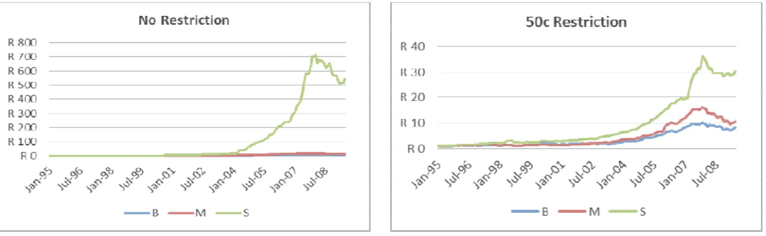
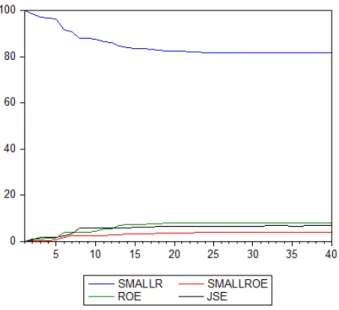
Figure 2: Size sorted portfolios restriction)

When sorting portfolios based on size

Rensburg and Robertson (2003a), Basiewicz and Auret (2009) and Strugnell, Gilbert and Kruger (2011). Figure 2 presents the results of a R1 investment in each of the size sorted portfolios sorted every 60 months

and Auret (2009) and Strugnell, Gilbert and Kruger (2011). The results indicate that a R1 investment in the extreme value portfolio at the beginning of the sample period would result end value of R140.38. When applying a price filter of 50c, the final investment for the extreme value portfolio is R33.17, which is consistent with the findin Basiewicz and Auret (2009) as they found that when applying a proxy for transaction c

, the value and size premium are diminished, yet throughout the value portfolio performs the growth portfolio. Interestingly, when using a three year holding period, the final value of a R1 investment in the extreme value portfolio results in a portfolio value of R211.25 with no price restriction applied, yet when applying a 50c restriction, the extreme value portfolio final value falls to R60.19 at the end of the sample period. When using a seven year holding period, the final value of the extreme value portfolio with no price restriction is R136.05. When applying the 50c price filter, the portfolio value drops to R50.33. The results seem to imply that the seven year filter achieves the lowest final value but also seems to be the least sensitive to a price filter as it experiences the lowest decrease when applying the price filter (See appendix 1 for the results of applying a 75c and 100c filter).

Size sorted portfolios using a 5 year holding period (No restriction and 50c

When sorting portfolios based on size, the results are consistent with the findings of Van Rensburg and Robertson (2003a), Basiewicz and Auret (2009) and Strugnell, Gilbert and 2011). Figure 2 presents the results of a R1 investment in each of the size sorted sorted every 60 months. The final investment value for the small cap portfolio over and Auret (2009) and Strugnell, Gilbert and Kruger (2011). The results indicate that a R1 at the beginning of the sample period would result . When applying a price filter of 50c, the final investment which is consistent with the findings of Basiewicz and Auret (2009) as they found that when applying a proxy for transaction costs , yet throughout the value portfolio Interestingly, when using a three year holding period, the sults in a portfolio value of R211.25 with no price restriction applied, yet when applying a 50c restriction, the extreme . When using a f the extreme value portfolio with no price restriction is R136.05. When applying the 50c price filter, the portfolio value drops to R50.33. The results seem to imply that the seven year filter achieves the lowest final value but also seems to be the least sensitive to a price filter as it experiences the lowest decrease when applying the price filter (See appendix 1 for the results

(No restriction and 50c

the results are consistent with the findings of Van Rensburg and Robertson (2003a), Basiewicz and Auret (2009) and Strugnell, Gilbert and 2011). Figure 2 presents the results of a R1 investment in each of the size sorted . The final investment value for the small cap portfolio over

(21)

the sample period, without considering liquidity and transaction costs, is R554.99. When accounting for liquidity and transaction costs, the final investment value of the small cap portfolio drops to R31.10. The incorporation of a proxy for transaction costs does not result in the disappearance of the size effect, therefore implying that there is a robust size and value effect on the JSE, and even when proxying for illiquidity and transaction costs, the small cap and value portfolios achieve superior returns when compared to the large cap and growth portfolios. Considering the results of the size sorts when applying a three year holding period, the small size portfolio final value is R511.92 while when applying a 50c filter, the value drops to R21.60. The seven year holding period results are even more interesting as the final portfolio value, when no restriction is applied is R399.37 and when applying a 50c filter the portfolio value drops to R32.63. The results seem to imply that an unrestricted size sort achieves a higher nominal return than a value filter yet the value sort is less sensitive to the application of a price filter. Another interesting finding is that the longer holding period sorts generally achieve lower final portfolio values yet are far less sensitive to the application of price restrictions. More importantly, the above evidence indicates that there is both a significant size and value effect on the JSE even when using abnormally long holding periods.

b) Vector Autoregressive Analyses (VAR)

VARs can be used to extract information from financial time series. Impulse responses determine the effect of a structural innovation or shock and its effect on a variable within an estimated system. Impulse response analysis may be based on the counterfactual experiment of tracing the marginal effect of a shock to one variable through the system. Stock and Watson (2001) stated that variance decomposition allows for the decomposition of the variation in a variable, given a shock or innovation experienced by another variable within an estimated VAR. A VAR is estimated for both the value and size sorted portfolio using the five year sorts. Since the time series data does not overlap, the five year sort is superior as the three year holding period is too short to be considered a “long” holding period, while the sample period only allows for two seven year sorts. In order to ascertain whether the VAR is stable and therefore whether the variables are stationary with in the VAR, a joint test of stationarity is run. For all variables considered within each of the VARs, all are stationary

(22)

and the VARs themselves are stable using both individual dickey-fuller GLS and combined tests of stationarity. Appendix 2 produces the graphical representation of the inverse roots of the characteristic polynomial. Since all the roots fall within the unit circle, this implies that all the variables within the VAR have roots that are less than one, indicating a stationary VAR.

For each VAR the basic equation estimated can be represented by

Where Ytis a vector of dependent variables including the monthly returns of the size sorted portfolios3, value sorted portfolios, the JSE ALSI return over the period, the ROE of the market, and finally the respective ROE’s of the size and value portfolios. The ROE of each share is calculated using the following formulae:

Xt is the clean surplus earnings per share. The same methodology is applied in order to derive a value weighted book value market index, from which the ROE of the market is derived (See Appendix 3 for the full derivation of ROE). Referring to equation 1, A0 is a vector of intercepts and Aqis a matrix of coefficients for each of the variables within the system lagged q periods. Finally, et is a matrix of the reduced form errors where errors are assumed to be uncorrelated and orthogonal. The VAR methodology assumes that each variable within the system is endogenous, consistent with the theoretical underpinnings of efficient markets and the CAPM, the only variables included are the respective returns of the individual portfolios and the returns of the market proxies. The time-series based tests are in effect a preliminary study on the time-series relationship between portfolio returns and their cash flow fundamentals proxied by ROE.

3

(23)

i. Impulse Response Functions

Impulse response functions are estimated for the extreme value and small size portfolios in order to determine the relative importance of innovations emanating from other variables within the system. It should be noted that the lag length selected for each of the VARs estimated was set to 12 months as Cohen, Polk and Voulteenaho (2008) found that only after a passage of time; are the first and second moments of share returns affected by cash flow fundamentals4.

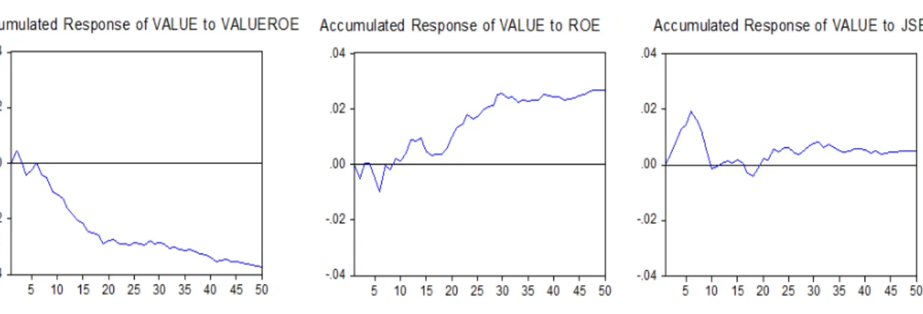
Figure 3: Impulse response function – 5 year value sort (50c restriction)

Impulse response functions were estimated for the value portfolio returns. The value portfolio returns over the entire sample period were set as the dependent or response variable. The VAR further included the time-series return of the JSE ALSI, the market based ROE and the corresponding time-series ROE of the value portfolio, sorted every 60 months. The above graphs indicate the marginal effects of a shock to the ROE of the value portfolio, the JSE ALSI and the ROE of the market on the return on the extreme value portfolio. An interesting result is that a shock to the corresponding ROE return of the value portfolio seems to have a negligible effect on the actual return achieved by the value portfolio. The graph indicates that there is a present initial shock however; the effect of the shock is decreasing over time.

4

One may take issue with such a methodology as one is generally bound to lag-length criteria tests, yet when utilising the proposed lag lengths, both the IRF’s and variance decompositions fail to identify a cash flow effect.

(24)

More interestingly, an innovation experienced by the overall ROE of the market has a significantly greater impact on the value portfolios return. The graph indicates that from 10 months post shock, a shock to the overall ROE of the market begins effecting the extreme value portfolio, emphasizing the long run effect of a cash flow shock. A corresponding shock to the JSE ALSI has a negligible effect on the value portfolios returns that only seems to fade 10 months post shock. The above findings imply that the returns of the value portfolio are more sensitive to innovations in the overall cash flow return of the market as opposed to actual price level return of the market proxy, strengthening the case for a cash flow based measure of systematic risk.

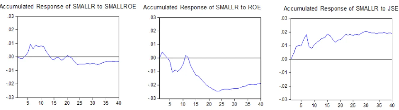
Figure 4: Impulse response function – 5 year size sort (50c restriction)

Figure 4 may give some insight as to why the cash flow beta appears less robust when attempting to explain the size effect. In contrast to the findings of Cohen, Polk and Voulteenaho (2008), a shock to the ROE of the market only seems to have an impact 25 months after the shock occurs and begins rising thereafter. A shock to the corresponding ROE of the small portfolio has a large initial impact which seems to die away after 25 months and only begins to increase at around 32 months post shock. Unfortunately, a shock to the JSE seems to have the most significant effect on the small size portfolio returns; implying that the small size portfolio is less sensitive to cash flow shocks of both its corresponding ROE and ROE of the market. The findings thus far indicate that a cash flow based measure of market risk seems more reliable in explaining the value premium and not the size effect.

(25)

ii. Variance Decompositions

The forecast error decomposition5 is the percentage of the variance of the error made in forecasting a variable due to a specific shock at a given horizon. The purpose of variance decomposition is to identify the variation of a variable given a current innovation of another variable. This allows one to identify the effect of an endogenous shock to the evolution of a variable in the system. Using the VARs estimated previously, variance decompositions are run.

Figure 5: Variance Decomposition – 5 year value sort (50c Restriction)

The above variance decomposition of the value portfolio returns is consistent with the impulse response functions. The graph indicates that a shock to the ROE of the market contributes more to the variation in the value portfolio returns than that of a shock to the JSE ALSI return. Once again a shock to corresponding ROE of the value portfolio has a minimal long term effect on the variation in the value portfolio returns. Moreover, the contribution of the value portfolio to its own variance is decreasing over time, consistent with the conclusion of Cohen, Polk and Voulteenaho (2008) that cash flow fundamentals begin dominating the

5

(26)

first and second moments of returns. The findings are interesting as they seem to confirm the evidence presented in the impulse response functions, as over long periods of time the variation in the value portfolios return is dominated by the ROE of the market.

Figure 6: Variance Decomposition – 5 year size sort (50c Restriction)

The results of the variance decomposition conducted on the small size VAR are marginally more promising than the results of the impulse response function conducted on the small size portfolio returns. The above graph indicates that the contribution of a shock to the small size returns contributes less to its own variance over time. Fascinatingly, the market ROE contributes slightly more to the variation in the small size return than that of the JSE. Given the results of the size VAR impulse response function, one would still question as to whether the cash flow beta proposed by Cohen, Polk and Voulteenaho (2008) can adequately explain the small size premium.

The above result should be interpreted with an element of caution, as the size portfolios effect on its own variation does not seem to decreasing with time as a shock at time 1 will still contribute to 80% of the variance of the size portfolio at time 40, and does not seem to be decreasing. Furthermore, a VAR is conducted assuming that the variables included are endogenous to the system; therefore the results do not cater for possible omitted variable bias.

(27)

A further caveat is in order as the lag length criteria tests were not employed as they suggested lag lengths of eight to nine months on average. Such a time span would naturally fail to capture the longer term innovations captured when the lag length is set to twelve months (Appendix 2)

c) VECM

Box and Jenkins (1970) described a method for dealing with data that are integrated of order one (“I(1)”). The methodology employs differencing in order to prevent the estimation of spurios relationships between economic variables. Engle and Granger (1987) and Johansen (1988) developed econometric models that use price levels or level data that is typically I(1) in order to estimate long run relationships between variables. The premise of the Engle – Granger and Johansen approach is that important information is lost when differencing time-series data. The purpose of the following estimated vector error correction models (VECMs) is to identify whether there is a consistent long-run relationship between the level returns of the value and size sorted portfolios and the book value6 of the market represented in levels. The results of the VECM estimations may provide further insight into the relationships between a value, size and cash flow. A further insight will be a comparison between the long-run relationship between the size and value portfolios and the JSE. A positive long-long-run relationship is expected between the book value based market proxy and the size and value portfolios. In order to strengthen the case for a cash flow based systematic risk measure, further tests are run by placing restriction on variables within both the cointegrating vector and the ‘speed of adjustment’ matrix. A restriction placed on the cointegrating vector, represented by β, implies the test of equal long-term relationships. The LR test provides insight as to whether two variables have equal long-term relationships with the independent variables. Another restriction test is employed where restrictions are placed on the speed of adjustment vector, represented by α. Such a restriction allows for the testing of whether a variable is weakly exogenous to the system. Similarly, the LR test determines if the restriction of weak exogeniety is binding. The failure to reject such a restriction would imply that the restricted variable does not actually adjust to the long-run equilibrium relationships prescribed by the VECM estimation.

6

(28)

i. VECM Methodology

In order to apply a VECM to the data, the data should be I(1). This presents an issue for the size and value sorted portfolios as value-weighted portfolio levels will be plagued by structural breaks. At each point of re-sorting, specifically over longer holding periods, the price levels of the value-weighted portfolios will fluctuate considerably, possibly resulting in inaccurate relationship measurements. In order to circumvent this issue, it is proposed that the equally-weighted levels be used. This implies that a fictional R100 investment7 is invested in each of the portfolios sorted on size and value. The resulting level time-series meet all the criteria required by the VECM model, specifically that the size and value portfolios are I(1) in the levels. Cointegration tests are run in order to identify the number cointegrating vectors in the VAR. In total, four VECMs are run where the level of the extreme size and value portfolios are included as well as the JSE level and book value of the market (otherwise referred to as the level ROE). Identification tests for cointegrating vectors are run. The tests utilise two Eigen value tests, namely the trace and rank test statistics that evaluate eigen values in order to determine the number of cointegrating relationships (see appendix 2).

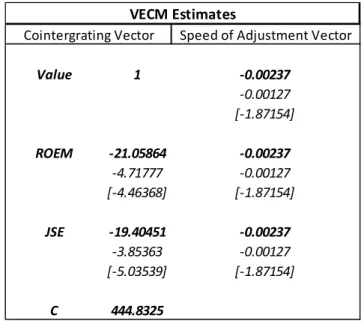
Table 1a: VECM output for the level ROE, JSE and Value portfolio (50c restriction)

7

R10 and R1 investments were also tested and the results were consistent

Value 1 -0.00237 -0.00127 [-1.87154] ROEM -21.05864 -0.00237 -4.71777 -0.00127 [-4.46368] [-1.87154] JSE -19.40451 -0.00237 -3.85363 -0.00127 [-5.03539] [-1.87154] C 444.8325 Cointergrating Vector VECM Estimates

(29)

The above VECM indicates that the cointegrating relationship is represented by the following formula:

! 444.84 21.06) 19.4+,

This implies that, as expected, the value portfolio seems to maintain a positive long-run relationship with the level ROE of the market where the ROE of the market is the monthly change in the value-weighted book value of the entire market inclusive of gross-dividends paid. A test for weak exogeneity is performed by imposing restrictions on the speed of adjustment vector (α vector). In order to test whether the ROE of the market is weakly exogenous to the system, the restriction is imposed setting α21 to zero. A rejection of such a test would imply that the ROE of the market is weakly exogenous to the system (refer to Appendix 2 – value VECM with restrictions β(1,1) = 1 and α(2,1) = 0). The LR test produces a p-value of 0.009, resulting in a rejection of weak exogeneity. To strengthen the case of a ROE based risk measure a further restriction is placed, where the cointegrating coefficient of the JSE is set equal to the ROEM (therefore β(1,2) = β(1,3)). The p-value produced by the LR test is 0.86, implying that one fails to reject the null hypothesis of the ROEM and JSE having(at least) an equivalent long run effect on the value portfolio.

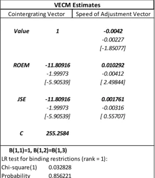
Table 1b: VECM output for the level ROE, JSE and value portfolio with restriction β12=β13

Value 1 -0.0042 -0.00227 [-1.85077] ROEM -11.80916 0.010292 -1.99973 -0.00412 [-5.90539] [ 2.49844] JSE -11.80916 0.001761 -1.99973 -0.00316 [-5.90539] [ 0.55707] C 255.2584 B(1,1)=1, B(1,2)=B(1,3)

LR test for binding restrictions (rank = 1): Chi-square(1) 0.032828

Probability 0.856221 Cointergrating Vector

VECM Estimates

(30)

A VECM is then estimated with the small size portfolio (in the levels) set as the dependent variable. A caveat should be mentioned about the size VECM. The results of the cointegration tests fail to reject the null hypothesis of no cointegrating relationships. In order to proceed with the testing, we assume that there is at least one cointegrating vector when estimating the VECM.

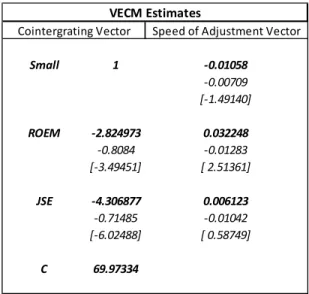
Table 2: VECM output for the level ROE, JSE and small size portfolio

The above results imply that both the book value market portfolio and the JSE have positive long run relationships with the small size portfolio. In order to determine whether the book value based market portfolio is weakly exogenous to the estimated system, the restriction of α21 equal to zero is set (refer to Appendix 2 – size VECM with restrictions β(1,1) = 1 and α(2,1) = 0). The LR test produces a p-value of 0.23, implying that the book value market proxy (that would be used to estimate cash flow beta and determine systematic risk) may be weakly exogenous to the system. When setting the cointegrating vector coefficients of the JSE equal to the book value market proxy, the LR test fails to reject the null, entailing that over the given sample period, it seems that the book value market proxy has an equivalently significant long run relationship with the size portfolio. This implies that the small size portfolio level returns have an equivalently long run sensitivity to the JSE as they do to the book value market proxy, implying that a cash flow based measure of systematic risk may perform as well as the conventionally measured CAPM beta that uses the JSE ALSI as a market proxy. Small 1 -0.01058 -0.00709 [-1.49140] ROEM -2.824973 0.032248 -0.8084 -0.01283 [-3.49451] [ 2.51361] JSE -4.306877 0.006123 -0.71485 -0.01042 [-6.02488] [ 0.58749] C 69.97334 Cointergrating Vector VECM Estimates

(31)

Another set of VECM estimations are run where the high minus low (HML) and small minus big (SMB) levels are used as dependent variables. The purpose of the tests is to ascertain whether the book value market proxy has an ‘as’ significant long-run relationship with the value and size premia (in the levels) when compared with the JSE.

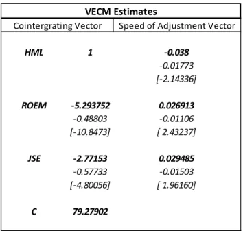
Table 3a: VECM output for the level ROE, JSE and HML level portfolio

As seen previously, both the book value market proxy and the JSE maintain positive long-run relationships. However when placing restrictions on the speed of adjustment vector parameters, the book value market proxy seems to be more weakly exogenous than the JSE. Table 3b: VECM Restriction results using SMB and HML as dependent variables

Dependent

Variable Restriction Chi-Square (1) p-value

A(2,1)=0 3.222155 0.072648 HML A(3,1)=0 4.597747 0.032014 B(1,2)=B(1,3) 6.725928 0.009502 A(2,1)=0 1.947768 0.162828 SMB A(3,1)=0 1.69832 0.192508 B(1,2)=B(1,3) 6.00849 0.014237 HML 1 -0.038 -0.01773 [-2.14336] ROEM -5.293752 0.026913 -0.48803 -0.01106 [-10.8473] [ 2.43237] JSE -2.77153 0.029485 -0.57733 -0.01503 [-4.80056] [ 1.96160] C 79.27902 Cointergrating Vector VECM Estimates

(32)

The above table indicates that when using the level excess return earned by the small size and high value portfolios, the test of weak exogeneity of both the book value market proxy and the JSE yields interesting results. When using HML as the dependent variable, the book value market proxy (A(2,1)=0) is weakly exogenous to the system yet, the JSE (A(3,1)=0) is not. Furthermore, the test for equivalent long-run relationships (B(1,2)=B(1,3)) is also rejected. When SMB is used, both the book value market proxy and the JSE are weakly exogenous to the system. When testing the equivalence of their long run relationships with the excess level return earned by the small portfolio, the LR test rejects the null of equivalent long-run relationships.

The above findings seem to be mixed as the book value market proxy seems to be effective as it maintains a significant long run relationship with the small size and value portfolios, however when attempting to explain the level excess returns earned by both the small size and high value portfolios, the book value market proxy seems to lack a significant long-run relationship with either, implying that the cash flow based measure of systematic risk proposed by Cohen, Polk and Vuolteenaho (2008) may not be the saviour of the CAPM.

E. Cross-Sectional Tests

Van Rensburg and Robertson (2003a) found that the CAPM beta fails to explain the size and value premium on the cross-section of average returns on the JSE. Strugnell, Gilbert and Kruger (2011) confirmed the results of Van Rensburg and Robertson (2003a) by testing different beta estimation techniques. The same conclusion was reached, namely that CAPM and beta in its current form, has a negligible (and possibly even an inverse) relationship with returns. Cohen, Polk and Voulteenaho (2008) suggested a method of estimating beta over extended periods of time, using the discounted change in book equity (referred to as ROE) and the overall discounted ROE of the market in order to calculate a cash-flow beta. As mentioned previously, ROE is defined as (See Appendix 3 for the full derivation of ROE):

_/0-.

.12 (2)