Internet Auctions with Many Traders
Michael Peters and Sergei Severinov
University of Toronto and University of Wisconsin
First Version Feb/01 This version June 8, 2001
Abstract
A multi-unit auction environment similar to Ebay is studied. Sellers who wish to sell a single unit of a homogenous good set reserve prices for their own independently run auctions. Buyers who hope to acquire a single unit bid as often as they like in a dynamic second price auction. When the number of buyers and sellers is large but finite, there is a Bayesian equilibrium for this completely decentalized trading procedure in which the ex post efficient set of trades occurs at a uniform trading price. Remarkably, the strategy rules that buyers and sellers use in this equilibrium are very simple. They do not depend in any way on beliefs, or on the number of buyers and sellers.
One of the central features of auction theory is the centralized nature of trade. Specifically, the seller, or auctioneer, establishes trading rules centrally processes information contained in messages sent by buyers and adjusts prices. Some recent examples include algorithms developed by Gul and Stacchetti (2000) and Ausubel (2000), both of which support efficient competitive trade as a Bayesian Nash equilibrium. Theory is less well developed in the case of mul-tilateral exchanges, like the stock exchange and some business to business sites on the internet, yet centralized processing of demand and supply information is a common feature.1 It is natural to think in these terms since standard
compet-itive reasoning is typically explained using a fictitious auctioneer who collects demand and supply information then uses some sort of tatonement process to compute market clearing prices.2
The theoretical literature that does exist on multilateral trade follows this lead by assuming that messages like bid and ask prices are centrally processed and used to compute efficient trades. Double auctions, for example Wilson 1For example, the NTE truck exchange (http://www.nte.net) allows truckers with excess carrying capacity to match with shippers who have small and unusual packages to send. The exchange does not use auctions, but instead uses what they call ’market based pricing’ to complete the trade. Apparently the ‘commodities’ used in this exchange are so narrowly defined that mechanisms similar to a double auction that use only demand and supply for a single ’commodity’ to determine the price attract too few buyers and sellers, so supply and demand information for related routes and times is aggregated and used to generate market prices.
(1985), are known to be incentive efficient. Rustichini, Satterthwaite, and Williams (1994) (following previous work by Satterthwaite and Williams (1089)) show that surplus lost by trading in centralized double auctions shrinks to zero very quickly as the number of traders gets large. Older experimental work by, for example, (Smith (1962)) seems to confirm these theoretical predictions.
At first glance, the trading technology offered by the internet appears to enhance this trend toward centralization since computers make it easier to as-semble and process large amounts of information. Large trading institutions such as Ebay,Ubid, and other business-to-business exchanges have emerged,3
and are growing quickly. For example, Ebay had 18.9 million registered users as of April 2001. Total sales volume at Ebay in 2000 was $ 5 bln. and this number is expected at least to double in 2001 (see Morneau (2001)).The volume of trade at business-to-business marketplaces has grown from $5 bln. in 1999, to $43 bln. in 2000 and, according to ActivMedia Research, is expected to reach $263 bln. in 2001 (see Wilson and Mullen (2000), Morneau (2001)).
On closer inspection, the notion that electronic trade promotes centralization of trade is less convincing. Though Ebay certainly presents a focal location for trade, Ebay itself does not do the processing of demand and supply information that occurs in a double auction, or in the single auctioneer mechanisms of Gul and Stacchetti (2000), orAusubel (2000). It is up to sellers to choose their own reserve prices and buyers to decide where to submit bids. Experienced traders apparently buy and sell in many locations. For example, it is possible to buy computers on Ebay, but they can also be purchased on line at suppliers own websites and at a variety of on line retail locations. Suppliers who do try to sell on Ebay, typically also offer their computers on other on line trading sites like Amazon, or Ubid.
The same technology that makes it possible to process large volumes of in-formation also promotes decentralized trade because it makes it possible for individual traders to collect dispersed information about prices and availability and react to it. For example, one could easily imagine that the robot guided bidding on Ebay could be carried out on a host or small private servers (owned by sellers) which simply enforced the trading rules used at the larger institution. Arguably the widespread use of relatively low power personal computers would seem to enhance decentralized decision making as much as it does central com-putation. This may be one reason that institutions like Ebay are so successful - they leave the responsibility for coordinating trade up to traders themselves.
Whether decentralized trade works or not depends on whether the algorithm used to compute prices and efficient trades can be broken up into bits that can be solved by individual traders, and whether traders have any incentive to follow the rules of the algorithm once this occurs. This issue has been addressed many times before, for example, it has been shown that in the context of random matching - bargaining may or may not produce competitive outcomes when trade frictions are small (see, for example, Rubinstein and Wolinsky (1990)). In 3The examples of large-scale business-to-business internet exchanges include CheMatch and Chem Connect (chemical industry), Covisint (auto parts), MetalSpectrum (aluminum, stainless steel, copper, iron, and other metals).
this paper, we extend this line of inquiry into an environment that has many of the characteristics of internet auctions and exchanges. Frictions are small and the appropriate way to match buyers and sellers is not obvious.
First, in regards to breaking up the algorithm into smaller parts, we allow sellers to (independently) run ascending price auctions similar to those that occur on Ebay. Buyers submit bids at these auctions, but when these bids are unsuccessful, we allow buyers to adjust their bids and move between sellers costlessly. We then provide a ’simple’ bidding rule that buyers can use to select among sellers’ auctions and choose their bids. This bidding rule uses information on publicly observable prices, and on the last bid submitted at each auction. Otherwise it is independent of buyers’ beliefs about the valuations of the other buyers and on the number of other buyers bidding. When buyers follow this bidding rule, all trades occur at a uniform price that coincides with the price in a ’sellers bid double auction’ where all bids and asks are processed in the centralized way4 and sellers’ ask prices are equal to their reserve prices. If the
sellers’ reserve prices happened to be equal to their true valuations, then the uniform trading price would be equal to the lowest market clearing price.
Then we show that the bidding rule that we specify constitutes a Bayesian Nash (continuation) equilibrium for buyers given the reserve prices of sellers. So not only does the algorithm parcel out the problem of computing equilibrium prices and trades, but buyers involved have the correct incentive to follow this algorithm.
In the second part of the paper, we show that there is a large but still finite number of buyers and sellers such that it is a Bayesian equilibrium for sellers to set their reserve prices equal to their true costs. So in this sense our decentralized market along with the simple bidding rule we describe for sellers always supports efficient trade at a uniform price when the market is large.5 So
the ’competitive outcome’ is completely decentralized.
The significance of the bidding procedure we descibe is not so much that it generates a competitive outcome, for it is known that there are many al-gorithms that will accomplish this. The algorithms described by Gul and Stacchetti (2000) and Ausubel (2000) are examples in the single seller case. Roth and Sotomayor (1990) describe an auction like mechanism that generates competitive trade in the environment we study. Demange (1982) and Leonard (1983) study the incentive properties of this mechanism. These procedure are not decentralized in the sense that ours is, since they require that a centralized auctioneer collect information and change prices6The interest in our procedure
4The sellers’ bid double auction is described in Satterthwaite and Williams (1089). 5We get stronger results in this regard than Rustichini, Satterthwaite, and Williams (1994) concerning the existence and efficiency of equilibria because we assume that there is a finite set of feasible valuations rather than a continuum. This assumption also allows us to get around the impossibility result of Myerson and Satterthwaite (1983).
6Roughly each buyer tells the auctioneer which sellers he would be willing to purchase from at the current set of prices. The auctioneer checks to see whether a matching of buyers to sellers is feasible given this information. If not prices are increased a bit at all the sellers where there is an excess demand. Buyers could send messages to each of the sellers in their ’demand sets’ informing them they are willing to trade, but sellers who have an excess demand can’t
stems from the fact that the price adjustments are done by traders themselves without any need for centralized intervention. The strategy rules that traders use to conduct themselves are simple. Buyers need to know only the current set of prices as well as whether or not the last bid with each seller (if there was one) was successful (in the sense that the buyer who submitted the bid became high bidder).
Apart from its theoretical value, this result has potentially important prac-tical implications since a decentralized market is less prone to technological failures7. We emphasize that our decentralization result does not require that
traders themselves carry out the sophisticated calculations that otherwise might have to be done by the mechanism designer intermediating the trades, or by buy-ers and sellbuy-ers attempting to foresee future trading prices in a rational expec-tations model. The strategies that buyers and sellers use ’work’ independently of the tastes, beliefs about costs or valuations and, for buyers, even the num-ber of traders who participate in the process. Thus, traders need very little information in order to carry out their equilibrium strategies.
Despite the fact that the market is completely decentralized in our model, the rules that govern exchange are very similar to the ones that are used on well-known internet auction markets since they are themselves quite decentralized. In this sense, our model gives some insight into the workings of markets like Ebay8 and other business-to-business marketplaces.
If bidders follow the strategies we descibe, predictable patterns of bids and pricing will emerge. For example, the winning bid in our model is not necessarily the last bid. However, because the bidders push up the standing bids slowly, the winning bid will normally be submitted towards the end of an auction. It would be rare in our mechanism for the winning bid to be submitted early in the auction (in the sense that there are many bids submitted after it). There is strong evidence that Ebay auctions are won by late bidders (Zheng (2001) or Roth and Ockenfels (2000)). High valuation bidders who follow Ebay’s advice to bid their true valuations early will win the auctions they participate in whether they bid early or late.
It is readily apparent in our model why buyers do not want to follow Ebay’s advice and bid their true valuations right away, leaving the robots to compute the prices later. Buyers who do so may be accidentally trapped into paying a higher price than they need to when a high valuation buyer bids against them. Incrementing the standing bid as slowly as possible (by submitting the minimum acceptable bid) avoids this.
tell whether a feasible match is possible or whether they should raise price without a signal from the auctioneer.
7The Toronto Stock Exchange for example, has suffered continuing technical problems that have shut down its computerized trading system repeatedly and resulted in millions of dollars in trading losses.
8ebay is a more centralized mechanism than the one we have in mind since the bidding is actually processed on ebay servers. It is not beyond the realm of possibility to imagine that sellers conduct the same auctions on their own servers. The boundaries of the market defined by the internet go far beyond the confines of a single server. Many companies who sell on ebay (sun computers is an example) use ebay as one of many different on line trading centers.
Another characteristic of the equilibrium is that winning bidders will tend to do more bidding than losing bidders (not necessarily all in the same auction). There is some preliminary evidence that activity and success are correlated consistent with our prediction. Our model predicts strong negative correlation between seller’s reservation price and bidding activity. Seller’s with high reser-vation prices should get few bids. However, at least to the extent that the commodities being sold are substitutes, our model also predicts that the units with high and lower reservation price should end up trading at the same price -so the correlation between trading price and the seller’s reserve price should be very weak.
There are (at least) two branches in the literature that are closely related to our paper. Our paper follows the lead of the literature on competing auctions McAfee (1993), Peters (1997), Peters and Severinov (1997), Hernando-Veciana (2000). The flavor of the results in that literature is similar to ours - when there are many competing auctions,equilibriumindirect mechanisms are independent of the characteristics of demand - second price auctions with reserve prices set equal to costs are bestmechanisms for sellers independent of their beliefs. We provide the same kind of result here since sellers use second price auctions and set their reserve prices equal to their costs (though sellers are only free to choose a reserve price in our model, they cannot use mechanisms other than auctions). The difference is that in the previous literature the cost of bidding is implicitly very high in the sense that buyers are able to submit only a single bid. As a consequence, the equilibrium outcomes in these models are not ex post efficient. Coordination problems are large enough that there are unrealized gains to trade. In our model bidders are allowed to submit as many bids as they like. In effect, this costless communication allows buyers to get around the coordination problems that arise in these earlier models.
We have mentioned already the connection between our work and the pric-ing algorithms of Gul and Stacchetti (2000), Ausubel (2000) and Roth and Sotomayor (1990). Our procedure is closer in spirit to the ’deferred acceptance’ algorithms of Gale and Shapley (1962) and Kelso and Crawford (1982) (the latter studies the case with transferable utility). These algorithms have the same decentralized feature that ours does in that proposal acceptance decisions can be left up to individual traders. It is known that the deferred acceptance algorithms are not information proof when utility is non-transferable. Less is known about the incentive properties of these algorithms with transferable utility. We do not address the incentive properties of this kind of algorithm in general, rather we focus on Bayesian Nash equilibria when the number of traders is large and valuations are drawn independently to show that efficient trade is supported.
Our arguments can be broken up into two parts. In the next section we de-scribe our model. This is followed with a description of the equilibrium strategies for buyers. Once we show that on the equilibrium path outcomes are equiva-lent to those that occur in a seller’s bid double auction, the analysis of sellers’ equilibrium strategies is then standard, but analytically demanding. In fact, our argument shows that sellers’ bid double auctions have efficient equilibria
when there is a finite set of valuations. This could be viewed as an independent contribution of the paper.
1
The Model
There aren sellers and mbuyers trading in a market. The number of buyers and sellers is arbitrary in our model, and we do not assume that there are more buyers than sellers. Each seller has one unit of a homogeneous good, while each buyer has an inelastic demand for one unit of this good. Buyers’ valuations and sellers’ costs are private information and are distributed on the grid D ≡
d, d+d, d+ 2d, . . . d that has a step size d > 0. Let F(·) and
G(·) be the probability distributions from which buyers’ and sellers’ valuations respectively are drawn. Our results on equilibrium bidding behavior by buyers are independent of whether or not buyers’ valuations are correlated, though our equilibrium for the sellers’ part of the game relies on independence. A buyer with valuation v who wins a single auction at a price p gets surplus v−p. A buyer who wins more than one auction gets no additional utility from the additional units of output (so his payoff will fall because he has to pay for the additional units). A sellers with costcwho sells at pricepget surplusp−c.
Trade is organized in the following way. At first, sellers simultaneously announce reserve prices for their auctions. Thereafter buyers arrive sequentially. When a new buyer arrives, he submits a bid at whichever of the sellers’ auctions he likes best. Buyers are required to submit bids in the gridD.9 The grid sized
could be thought of as the minimum bid increment. When the seller receives a bid, she publishes a number called herstanding bid which is equal to the second highest bid that she has received, or her reserve price if she has not received more than 1 bid. Each seller immediately updates her standing bid announcement when her standing bid changes. As in most existing on-line auctions, we also assume that the identity of the winning bidder is known at all times10.
We assume throughout that the second-highest bid means second highest bid submitted by a distinct bidder. The standing bid is assumed to remain unchanged if the high bidder revises his bid. A new bid submitted at a seller’s auction must always exceed that seller’s current standing bid. If two or more bidders have submitted the same high bid, then the buyer who was the first to submit this bid is declared the high bidder. The standing bid in this case is equal to the high bidder’s bid.
After a new bid is submitted, each buyer in order of his or her entry into the market is given the opportunity either to submit a new bid (not necessarily with the same seller) or pass. Once each buyer in the market chooses to pass, a new buyer enters. After all buyers have entered the market, the bidding process 9This assumption is natural in view of our interpretation that the grid on which the traders’ valuations are distributed is determined by the minimal monetary unit.
10As will be show later, this assumption, or more precisely, the observability of the change in the identity of the winning bidder is important for the uniform price result. When such changes are not observable, price dispersion may occur
continues as bidders update their bids one after another. The order of bidding at this stage is the same as the order of entry with the last bidder followed by the first bidder and so on. The bidding continues until all buyers pass. Then the high bidder at each seller trades at the final standing bid with that seller.
These rules approximate the trading rules on Ebay and on the Amazon auction site (which differs from Ebay primarily in that auctions do not have a definite ending date (see Roth and Ockenfels (2000))). The key property of the auction rules is that they generate a type of the second price auction in which the high bid is never observed.
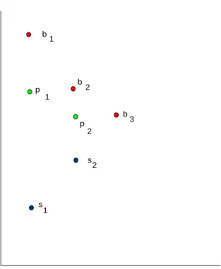
Despite the second price nature of the auction mechanism, the presence of multiple auctions implies that it is not a dominant strategy for buyers to bid their true valuations when they start bidding (despite the advice offered on the ebay website). To see this, consider the data in Figure 1. For the moment, ignore the pointb3, and suppose that there are two buyers with true valuations
b1 andb2 and two sellers who announce reserve pricess1 ands2. Assume that the buyer with valuationb1 enters first and expects the other buyer to bid his true valuation wherever he decides to bid.
To show that it is not a dominant strategy, we only need to show that valuation bidding can be strictly improved upon forsome strategy of buyer 2, so suppose that buyer 2 is expected to bid his valuation where the standing bid is lowest. Buyer 1 could bid her valuation with seller 2. She should then expect buyer 2 to bid his valuation with seller 1 who has a lower reserve price. No matter what bid buyer 2 submits, buyer 1 will trade at price s2. Buyer
1 can strictly increase her expected payoff by initially bidding s2 at seller 1,
provided she believes that buyer 2 has a valuation belows2with strictly positive
probability.
So if buyer 1 is going to start off bidding her valuation, she will bid with seller 1. When buyer 2 enters, the standing bid with seller 1 remains at s1
because seller 1 has yet to receive a second bid. So by the rule that buyer 2 is supposed to be using, buyer 1 should expect buyer 2 to bid against her provided he bids at all.
If buyer 2 bids at or belows2, then buyer 1’s initial strategy works out fine, and she trades at a price at or below s2. If buyer 2 submits any bid above
b2, then buyer 1 will be displaced as high bidder, and will trade at price s2
with seller 2 - again a reasonable outcome. The difficulty arises when buyer 2 submits a bid strictly aboves2 but strictly below b2. In this case, buyer 1
will pay a price strictly above s2. It is not hard to see that if buyer 1 starts
with a bids2 with seller 1 (instead ofb1), then everything works out the same
way, except that when buyer 2 bids something between s2 and b1, buyer 1 is
displaced as high bidder and trades at prices2 with seller 2. Deviating to the
price s2 ensures that buyer 1 will never have to pay a price above s2. This strictly improves upon the bidb2 provided buyer 1 believes that buyer 2 has a valuation betweens2andb1with strictly positive probability.
v n b 1 b 2 b 3 1 s 2 s Figure 1:
2
Efficient Bidding
The advantage of sequential bidding is that buyers whose valuations are high, but who had the bad luck of bidding against another buyer with an even higher bid, have an option to bid again elsewhere. Unfortunately, this option is not sufficient to guarantee that, conditional on seller’s reserve prices, the efficient trades are carried out. The following example demonstrates this.
In Figure 2, given sellers’ reserve pricess1ands2the efficient outcome is for
buyer 1 to trade with seller 1. However, consider the following strategies. If a buyer finds that no other bids have been submitted and his valuation is at least
s1, then he submits a bid equal tos2 with seller 1. If there is a bid at seller 1, then the buyer bids his valuation with seller 2 provided his valuation is at least as large ass2, and refrains from bidding otherwise. This strategy is optimal for the buyer who enters first because she ends up trading with seller 1 at prices1. Following this strategy is also optimal for the buyer who enter last, because he believes (correctly) that the buyer who has already entered has bids2 at seller
v n b 1 b 2 1 s 2 s Figure 2:
1. Therefore, there is an equilibrium in which both buyers use this strategy. Given the data in Figure 2, if buyer 2 enters first then in this equilibrium he will trade with seller 1, and then buyer 1 with a higher valuation will trade with seller 2. Thus, equilibrium outcome of the bidders’ game could be inefficient.
It is easy to demonstrate that in this example, as well as in many other ones, the dynamic bidding game has multiple equilibria. We will not attempt to char-acterize all of them. Rather, our objective is to try to identify bidding equilibria that have nice properties, especially, the ones that are efficient conditional on the announced reserve prices.
To begin, let b ={b1, . . . bm} be the vector of buyers’ valuations, and let
s={s1, . . . sn}be the vector of sellers’ reserve prices. Without loss of generality,
assume that sellers are indexed in such a way thats1≤s2· · · ≤sn, while buyers
are indexed the opposite way so thatb1≥b2· · · ≥b3. Following Satterthwaite and Williams (1089), letv={v1, v2, . . . vm+n}be vector with entryvi equal to
i-th lowest value among buyers’ valuations and sellers’ reserve prices. If sellers’ reserve prices were equal to their true valuations, then the efficient set of trades
occurs if buyers whose valuations exceed vm trade with sellers whose reserve
prices are equal or less than vm. To see why, note that initially there are n
sellers holding one unit of output and m buyers. Therefore, after all trades are completed exactly n traders will own the good and the other m will not. Efficiency requires that the traders who end up without the good have the lowest valuations or costs.
We now define the symmetric strategy σ∗ by specifying how each buyer should bid when his (her) turn comes. To help describe the strategy, make the natural definition and say that a bid is successful if the bidder who makes it becomes high bidder, and that the bid isunsuccessful otherwise.
Definition 1 The symmetric strategy σ∗ is defined as follows: if it is the buyer’s turn to bid then
(a) if the buyer is the current high bidder at any auction, or if the buyer’s valuation is less than or equal to the lowest standing bid, the buyer should pass;
(b) otherwise, if there is a unique lowest standing bid, the buyer should submit a bid with the seller offering this lowest standing bid. The bid should be equal to the lowest value on the grid that exceeds this low standing bid;
(c) otherwise, if more than one seller has the lowest standing bid, the buyer should submit the same bid as in (b) with equal probability at each such seller where either the seller has not recevied a bid, or the last bid the seller received was unsuccessful. If the last bid was successful with all sellers holding the lowest standing bid, then the buyer should bid with each of them with equal probability.
Before proceeding, it might help to visualize the path generated when buy-ers use strategyσ∗ in a simple demand-supply style diagram. We refer again to Figure 1, where the valuations and reserve prices of three buyers and two sellers are shown. This is simply an example designed to illustrate the way the strategies work, so for convenience we can assume that the grid of feasible bids coincides with the set of sellers’ reserve pricess1, s2and buyers’ valuations
b3, b2, b1. Assume further than buyers enter in reverse order of their valuations,
so buyer 3 with valuationb3 enters first, then buyer 2 then buyer 1. According
to strategy σ∗, when buyer 3 enters he bids s2 with seller 1 because seller 1
initially has the lowest standing bid and s2 is the lowest valuation on the grid
that exceedss1. This bid will be successful but it will have no effect on seller
1’s standing bid. Buyer 2 will bid the same amount with seller 1, since seller 1’s standing bid still has the lowest standing bid.
The bid by Buyer 2 is unsuccessful, but it makes the standing bid with seller 1 rise tos2. Observe that unsuccessful bids will always change a seller’s standing bid, since buyers must submit bids above the current standing bid. As buyer 3 was the first to submit this bid, he remains the high bidder and passes by (a), so buyer 2 has the chance to submit a new bid. Now both sellers have the same
standing bid. The last bid with seller 1 was not successful, and seller 2 has not yet received a bid. The lowest value that exceeds the standing bids2 isb3, so by (c) buyer 2 will bidb3 with equal probability at seller 1 (case (a)) or seller 2 (case (b)). In either case, buyer 2’s bid will be successful and it will not affect either of the standing bids. Note that a successful bid may or may not change a seller’s standing bid.
Consider case (a) first. Since buyer 2 displaces buyer 3, buyer 3 immediately submits a bid equal tob3with seller 2, since seller 2 has yet to receive a bid in
this case. The bid is successful, and again, this bid does not affect either of the standing bids which remain equal tos2. When buyer 1 enters he finds that
the last bid with both sellers was successful, so he will randomize. Whichever sequence he chooses, the bidb3will be unsuccessful and will raise the standing bids at both sellers will rise tob3. Then buyer 1 will bidb2 choosing randomly between the two sellers (since the last bid was unsuccessful at both locations). If buyer 1 bids first with seller 1, then he will displace buyer 2, who will, in turn, bidb2 at seller 2 and become a winning bidder there. Bidding will then stop, and buyers 1 and 2 will trade at priceb3. If he bids first with seller 2, his bid will be successful and all bidding will stop.
Now consider case (b). When buyer 1 enters, he will submit bidb3 at seller 1 and displace bidder 3 without raising the reserve price above s2. Buyer 3
will then submit bidb3 at sellers 1 and 2 in random order, which will raise the
standing bid at both sellers tob3, but bidder 3 will still not be a winning bidder.
The bidding will then stop and buyer 1 and 2 will trade.
This example conveys the essential idea. Buyers bid up prices with each seller as slowly as possible. For this reason, high valuation buyers are never trapped into paying higher prices if another high-valuation buyer accidentally bid against them. In this example, the efficient trades occur and both sellers trade at a uniform price equal to buyer 3’s valuation. The randomness on the equilibrium path makes possible different profiles of winning bids and different pairwise matching between buyers and sellers who trade. However, the uniform trading price is uniquely determined by the profiles of buyers’ valuations and sellers’ reserve prices. These properties of the strategy ruleσ∗are quite general, as the following theorem demonstrates.
Theorem 2 The outcome in which all buyers use the strategy σ∗ is a perfect Bayesian equilibrium. For each array of valuations and reserve prices v, each buyer whose valuation is above vm trades with some seller whose reserve price
is no larger thanvm. All trades occur at the pricevm.
The proof of this and the other main theorems in the paper is included in the appendix.
According to strategyσ∗, all active buyers focus their bids on seller(s) with the lowest standing bids irrespective of buyers’ valuations, beliefs and the stand-ing bids. The active bidders continue to bid up the standstand-ing bid with this group of sellers (which could consist of only one seller) until their standing bids reach
the level of the standing bids or reserve prices at the next group of sellers, i.e. the second lowest level. Then bidding continues with sellers from both groups until the lowest standing bid reaches the level of reserve price or standing bid at the next group of sellers, and so on. This process continues until all remaining active bidders become high bidders with different sellers.
It is notable that strategyσ∗ contains the same set of rules on the equilib-rium path as well as off the equilibequilib-rium path. But, although σ∗ generates a relatively simple path, the proof that playingσ∗ constitutes an equilibrium is not straightforward because the dynamic bidding game is sufficiently complex. We provide the proof by showing that a buyer who at any stage of the bidding game submits a higher bid than what is prescribed byσ∗, or who bids above his valuation can at best raise the trading price. At the same time, a buyer who bids as if his valuation is lower than what it is in reality, can sometimes lower the trading price, but only by giving up a desirable trading opportunity.
This line of argument is similar in spirit to the one that is used to show that bidding the true valuation is an equilibrium in a standard static second price auction. But the analogy is only approximate.11 A substantially more complex argument is needed because of the dynamic nature of the bidding process and presence of multiple auctions. To compute the payoff that a buyer gets by followingσ∗from the outset of the game, as well as the payoffs that he could get by deviating, we need to consider arbitrary information sets and characterize the outcomes that occur after the play of the game has reached them. In particular, we need to show that playingσ∗ remains optimal for a buyer no matter what information set is reached, if in the continuation all other buyers followσ∗.
An important property of the equilibrium where buyers useσ∗is absence of price dispersion in the final outcome: all trades are executed at the same price. Rule (c) inσ∗plays the crucial role in achieving this. This rule describes buyers’ behavior when there are several sellers with the lowest standing bid, and so the buyer faces the uncertainty regarding the winning bids at these sellers.
The essence of rule (c) is that it allows the buyer to identify which of the sellers with the same standing bid have lower winning bids. Bidding only at such sellers is optimal for the buyer, because then with some probability the buyer will trade at a lower price. At the same time, such bidding ensures that standing bids rise uniformly and eliminates the possibility of price dispersion.
Rule (c) tells the buyer to focus on such sellers with lowest standing bids where there had been less action at the current standing bid, or more precisely, where the last submitted bid was unsuccessful in the sense that the bidder who submitted it did not succeed in displacing the high bidder at the auction. On the path generate by our strategies, a successful bid will be strictly above the standing bid and will displace the lead bidder without changing the standing bid. An unsuccessful bid will raise the standing bid without displacing the winner. Thus, when two standing bids are the same, the one where the last bid was successful will have a larger high bid.
11As shown above, bidding one’s valuation is not an optimal strategy in the dynamic bidding game.
For each arrayvof buyers’ valuations and sellers’ reserve prices, theorem 2 uniquely specifies the price at which all trades will be completed. Precisely, the trading price will be equal to vm which is either the highest valuation among
buyers whose bids are unsuccessful, or the highest reservation price among sell-ers who trade, depending on the actual array of valuations and reserve prices. At the same time, the randomization on the equilibrium path (buyers random-ize between the sellers among whom they are indifferent) implies that certain aspects of the outcome will also be random. First, the final matching between sellers and buyers who trade is going to be random. Second, if there arek >1 traders whose valuations or costs are equal to vm, then any number of them
between zero tok−1 may trade in equilibrium.
To better understand whether buyers and sellers with valuations and costs equal to vm trade, let us divide the set of buyers into three groups. For any
array v, let M1 be the set of buyers whose valuations are strictly lower than
vm,M2be the set of buyers who have valuationsexactly equal to vm, whileM3
be the set of buyers whose valuations arestrictly higher than vm. Similarly, let
N1, N2, andN3 be the sets of sellers who set their reserve prices below, equal to and abovevm respectively. Letmi (ni) be the number of buyers (sellers) in
the setMi (Ni). Theorem 2 says that buyers inM3 will surely trade, and that
buyers inM1 and sellers fromN3 will not trade.
Corollary 3 Let vmbe the m-th lowest element in the arrayvof buyers’
valu-ations and sellers’ reserve prices. If all buyers use the strategyσ∗ in the bidding game, a seller who sets reserve pricess.t. s < vm trades for sure. The number
of sellers with reserve price equal tovm who trade trade is between
max [0, m3−n1] and min [n2, m3−min{0, n1−m2}]
The number of buyers with valuation equal tovm who trade is between:
max [0, n1−m3] and min [m2, n1−min{0, m3−n2}]
Proof: see the appendix.
Since all sellers fromN2(buyers fromM2) are identical, they have the same
chances of trading. Therefore the probability that a seller fromN2(buyer from
M2 trades lies in the interval with boundaries that are derived by dividing the corresponding boundaries on the number of sellers fromN2 (buyers from M2) who trade overN2 (M2).12
12By modifying the definition of strategyσ∗ appropriately, we can support equilibria in
which the number of sellers fromN2who trade is equal to the lower or upper bound established in corollary 3. To obtain the lower bound, modifyσ∗in the following way. When a buyer faces the choice between several sellers who have the lowest standing bid and who are equivalent with respect to rule (c), he bids at first with those sellers whose original reserve prices were lower than their current standing bid. Then the buyers inM3will submit bids with sellers in
N1before they will consider the sellers inN2. When the opposite modification on the strategy
σ∗is imposed, we can support an equilibrium that reaches the upper bound on the number of sellers fromN2who trade.
The central implications of the corollary 3 is that the outcome of the bidding game is efficient: traders who are left without the good at the end of the day are the ones who have the lower valuations and costs. Note that no matter how many sellers fromN2and buyers fromM2trade, this has no effect on the other traders and the efficiency of the outcome.
We view the presence of randomness in the final outcome as a strength of our model. In large decentralized markets it is unrealistic to expect all aspects of the bidding process to be entirely deterministic. Yet, we demonstrate that despite the presence of randomness on the equilibrium path, the final price will be uniform and independent of the actual path of bidding.
It is also worth pointing out the connection between our result and equi-librium in the double auction market. Consider a double auction with uniform trading price set equal to m-th lowest value among buyers’ bids and sellers’
asks. Satterthwaite and Williams (1089) refer to it as ‘seller’s bid double auc-tion’. They show that buyers would bid their true valuations in it and therefore, conditional on the seller’s ask prices (reserves), the trading price will be equal to vm. Bidding his valuations is optimal for a buyer because his bid can only
affect the trading price if the buyer fails to trade. The usual second price logic then implies then applies. Thus, the dynamic bidding game studied here has an equilibrium that generates an outcome identical to the outcome in a seller’s bid double auction when sellers’ reserves prices are the same set in both markets.
Concluding the discussion of the bidding game, note that neither the de-scription of strategy σ∗ nor the proof that σ∗ is a best reply depends in any way on the distribution of valuations, or the number of buyers and sellers in an auction.13 For example, if there is only a single seller, the trade will occur
at the reserve price if there is only a single buyer whose valuation is above the reserve, and at the second highest valuation otherwise. This is the same as the outcome in a second price auction. Playing strategyσ∗ remains an equilibrium when there is a large number of sellers. On the other hand, as in the seller’s bid double auction, a seller’s behavior in our mechanism will typically depend on her beliefs and the number of traders. We turn to the this issue in the next section.
3
Sellers’ Strategies and the Efficiency Result
The results of the previous section indicate that buyers’ equilibrium strategies guarantee that the efficient set of trades occurs when sellers set reserve prices equal to their true valuations. Buyers behavior is efficient because buyers affect the trading price only when they forego attractive trading opportunities.
At the same time, the outcome will not necessarily be efficient if sellers 13This statement has to be qualified slightly since we impose restrictions on beliefs off the equilibrium path, for example to ensure that no buyer believes that the high bidder in a any auction has a valuation below the standing bid in that auction. This restriction may seem unreasonable if valuations are correlated and prior beliefs conditional on the buyer’s own valuation are inconsistent with this.
set reserve prices that are different from their true costs. So we turn to an examination of sellers’ behavior in this section.
It may not be optimal for a seller to set a reserve price equal to her true valuation, because her reserve price may affect the trading price in some cases. For example, consider the situation depicted in Figure 1 without buyer 3 (the one with the lowest valuation). From the Figure it is clear that, if buyers use strategyσ∗, the uniform trading price will be equal to the higher reserve price as long as it is below b2. Sellers, of course, do not know b2. Thus, seller 2
could raise the trading price with a strictly positive probability by raising his reservation price aboves2. Clearly, the cost of increasing her reserve price to
seller 2 is that she would fail to trade if either buyer has valuation betweens2
and her new higher reserve price.
This tradeoff is similar to the one which traders face in a standard double auction. The rate of convergence of the optimal reserve prices to their true costs in a double auction has been analyzed by Satterthwaite and Williams (1089) in the case where the costs and valuations are independently and continuously distributed over an interval. In the analysis below, we will also maintain the independence assumptions. However we consider a finite grid of valuations which allows us to get a somewhat tighter result.
Thus, assume that buyers’ valuations and sellers’ costs are distributed inde-pendently. Letf(p)≡F(p)−F(p−1) andg(p)≡G(p)−G(p−1) denote the probability that a buyer’s valuation and a seller’s cost respectively are equal to
pexactly. Let ¯g= minp∈Dg(p) and ¯f = minp∈Df(p). We further assume that ¯
g >0 and ¯f >0.
We consider a sequence of markets that get larger as the number of traders increases. For simplicity, we hold the ratio of the number of buyers to the number of sellers constant at k > 0 i.e., m = kn where m is the number of buyers andnis the number of sellers.
The main result of this section is the following theorem which establishes that setting a reserve price equal to the true cost constitutes an equilibrium strategy for sellers when the number of traders in the market is sufficiently large.
Theorem 4 Suppose that every seller except sellerzsets her reserve price equal to her true cost and buyers follow the strategy σ∗. Ifm andn are sufficiently large, it is optimal for sellerz to set reserve price equal to her true cost.
The proof of this theorem is provided in the appendix. It demonstrates that, provided that the number of traders is sufficiently large, a seller with cost
cobtains a higher expected payoff by setting reserve price equal top−drather thanp for p > c. The two expected payoffs are the same if the trading price is either above p or below p−d. Thus, we need to focus on the situations where sellerj’s choice betweenpandp−daffects the trading price, and where the trading price is equal to p−d or p irrespective of seller j’s choice. The latter situation occurs if several other sellers post the reserve price equal to the trading price. The probability of this event is zero when the costs are
distributed continuously. Yet, with a discrete set of valuations it occurs with a positive probability and has an important effect. When several sellers are tied at the trading price, a seller may fail to trade even if her reserve price is equal to the trading price, because of the competition from the other sellers posting this reserve price.
Precisely, sellerjgets different expected payoffs by setting reserve price equal top−dor pin the following four cases:
1. the trading price is equal top−dwhether the seller sets her reserve price equal top−dor p, and sellerj trades after setting pricep−d.
2. the trading price is equal top−d(p) when the seller sets her reserve price equal top−d(p) and the seller fails to trade at pricep14.
3. the trading price is equal to p whether the seller sets her reserve price equal top−dorp, and sellerjfails to trade after setting reserve price p. 4. the trading price is equal top−d(p) when the seller sets her reserve price
equal top−d(p) and the seller trades at pricep.
The seller gets a higher expected payoff by setting reserve price equal to
p−dif the effects of (1)-(3) outweigh the effect of (4). In the proof, we ignore the effect of (1) and (2) and show that the effect of (3) alone dominates (4). The effects of (1) and (2) are ignored because whenp−d=c, the net surplus to seller j from trading at price p−d is zero. Comparing (3) and (4), we can reinterpret our findings as follows: a seller posting pricep−d has higher chances of trading at pricep than a seller posting pricep. To understand the intuition behind this result, note that the expected number of sellers posting a reserve price equal to the trading price increases as the number of traders grows. Competition from these sellers implies that with a significant probability a seller posting such reserve price fails to trade. Yet, if this seller posts a reserve price that is slightly lower than the trading price, she will trade with probability 1 and obtain a positive surplus.
4
Conclusion
At least two remarks are in order about the results of this paper. First, the equilibrium in buyers’ bidding game that we describe is not unique. Although the behavior that occurs in our equilibrium is plausible, alternative equilibria exist and do not generally guarantee efficient allocations. Examples in the paper illustrate this. We do not have a complete characterization of all equilibria in the dynamic bidding game, and of sellers’ optimal behavior with respect to reserve prices when they believe that buyers are to play a different equilibrium.
Part of the job of an equilibrium in a decentralized market is to coordinate the matching decisions that buyers and sellers make. Coordination problems 14It is easy to show that sellerjwill always trade after posting reserve pricep−din this case
almost always have multiple equilibria and having to choose among them seems inevitable. Second-price auctions, for example, possess asymmetric equilibria in which bidders do not bid their true valuations. There are multiple equilibria in centralized mechanisms like double auctions as well.
Taking the multiplicity problem seriously, we do not want to suggest that traders will play the equilibrium described in this paper under all circumstances. At the same time, the equilibrium behavior that we identify has a number of advantages. It is reasonable-looking, i.e. simple, requires very little computation on the part of traders, and is invariant to the form of the distributions from which costs and valuations are drawn. It also implements the efficient allocation. These properties make us believe that this equilibrium has focal nature, and eventually traders will learn to play it.
Of course, our model does not reproduce all details of the bidding behaviour on the ebay, Amazon or other auction sites. These auctions typically possess additional dynamic aspects that we do not consider. For example, sellers enter at random times, as do buyers. Auctions close at different times. Furthermore, bidding is not completely costless on these sites. Roth and Ockenfels (2000) suggest network congestion and unexpected demands by the family as reasons why bidders may not be able to revise a bid as intended. Nonetheless, our model does provide some insight into the workings of these institutions.
As mentioned above, our model gives a very simple explanation for the fact that buyers do not bid their true valuations. Patient revision of bids provides buyers with the signals that they need in a decentralized market to coordinate their bidding behavior. Deviating from this pattern will often force a buyer to trade at a price that is higher than necessary. The empirical implications of our theory are discussed in the introduction. An extension of the logic of our model suggests an explanation for observed flurry of active bidding close to the end dates in the ebay auctions. In our model, all the available trading opportunities are visible at the beginning of the bidding process. On ebay, these opportunities arise at random times. One of the opportunity costs of submitting a bid on ebay arises from the possibility that a new seller will enter at a lower reserve price after the buyer submits his bid. The buyer may then end up trading at a higher price than he needs to. Effective coordination of bidding among buyers then demands that they refrain from starting the bidding as long as possible. Since auctions at ebay have fixed end dates, at some point the probability that new sellers will enter before the current auction ends becomes small, and buyers will start bidding. One of the implications of our theory is that this late bidding on an auction that is ending will induce a flurry of bidding at other auctions for similar goods.
5
Appendix
Proof of Theorem 2:
At first, let us introduce the following notation. Let thestate of the game be the array of buyers’ valuations, sellers’ standing bids together with the
iden-tities of buyers who have submitted them, the winning bids together with the identities of the winning bidders, the history of the standing bids and winning bids, plus the identity of the buyer who is the next to move, and the order in which buyers will move in the continuation. Typical state of the game will be denoted by Γ. Note that there is a one-to-one relationship between the nodes in the game and states of the game. Precisely, state of the game is a full de-scription of the situation at the corresponding node in the game. Definepublic state of the game as the components of the state of the game that are publicly known. Specifically, public state of the game includes the standing bids, the winning bids, the identities of the winning bidders, the history of all these, and the order of moves.
We will say that state of the game Γ is regular if every buyer’s valuation is at least as large as any high bid that he holds at Γ. Note that whether the state of the game is regular or not is unobservable.
We will say that bidder i’s position isconsistent with σ∗ if each ofi’s high bids has the following property: ifiis a high bidder with sellerj then either (i)
i’s bid is one grid point above sellerj’s standing bid and no seller has a lower standing bid than does sellerj; or (ii)i’s high bid is equal toj’s standing bid. It is not hard to see from the definition that on the path generated byσ∗all states of the game are regular, and that every buyer’s position in these information sets will be consistent withσ∗.
If in state Γ one or more buyers are high bidders at more than one seller, we will replace the continuation of the true game from the node that corresponds to Γ with the one where additional ’phantom’ buyers are added to the game, but where each buyer (real or phantom one) has a winning bid at one seller at most. The phantom buyers are added in the following way. If buyer i is a winning bidder at multiple (say,l >1) sellers, choose any one ofi’s highest winning bids and consider that buyeri possesses only this winning bid. For each ofi’s l−1 other high bids, create a phantom buyerik (2≤k≤l−1) whose valuation is
equal to this winning bid. Then, define ˜vto be the vector of the valuations of the real and phantom bidders, and the current standing bids in state Γ. If there are ˜m≥mbuyers and phantom buyers, then ˜vhas dimension ˜m+n. Let ˜vris
ther-th smallest element of vector ˜v.
Define BΓ to be the smallest set of buyers (including phantom buyers) at state Γ such that ifBΓ containsmΓ bidders, every buyer who is not in BΓ is
high bidder with a seller whose standing bid strictly exceeds ˜vmΓ.
Lemma 5 If state of the gameΓ is regular, then the setBΓ is non-empty and
unique. Furthermore ifBΓ containsmΓ buyers, no buyer inBΓ is high bidder
at a seller with standing bid above˜vmΓ.
Proof. LetB0 be the set of buyers who are not high bidders at any seller. Suppose that B0 includes τ0 buyers. By definition, B0 ⊂ BΓ. Let s0 be the lowest standing bid. If ˜vτ0 < s0thenBΓ =B0, and we are done. Otherwise,BΓ
must containall buyers who are high bidders at sellers with standing bids0. To see this, consider any candidate setB1 with τ1 ≥τ0 members which contains
B0. Since ˜vτ1 ≥v˜τ0 ≥s0, a high bidder ats0 does not satisfy the condition for
exclusion fromB1.
We can now apply the same argument recursively. Let Bl be the set that
includes all buyers fromB0 and all buyers who are high bidders at the lowest, second lowest, ...,l-th lowest standing bids. Suppose that there areτlbuyers in
Bl, and no subset ofBl satisfies the definition ofBΓ. If ˜vτl < sl+1, wheresl+1 is thel+ 1-th lowest standing bid, thenBΓ=Bl. Otherwise,BΓ must contain
all buyers who are high bidders with sellers whose standing bids are less than or equal tosl+1. Continue in this way untill0 s.t. Bl0 satisfies the definition of BΓ or until all buyers have been included inBΓ.
It is immediate that no buyer inBΓis a high bidder at a seller whose standing bid exceeds ˜vmΓ (where mΓ is the number of bidders in Γ), for such a bidder
can be excluded fromBΓ to form a strictly smaller set satisfying the definition.
v n b 1 b 2 b 3 1 s 2 s p p 1 2 Figure 3:
Figure 3 provides an example of a situation with phantom bidders. Buyers’ valuationsb1, b2, b3 and sellers’ reserve pricess1, s2 are the same as in Figure 1.
However, in the state which we are considering buyer 1 has submitted two high bids,p1 with seller 1 andp2=b3 with seller 2, but no other buyer has entered yet. The standing bids remain s1 at seller 1 and s2 at seller 2. Since buyer 1 is high bidder at two sellers, we generate a phantom buyer whose valuation and bid are both equal top2. There are then 4 buyers including the phantom buyer, instead of only 3 in the original game). The vector ˜vof valuations and standing bids in increasing order is given by (s1, s2, p2, b3, b2, p1, b1). BΓ is the
whole set of buyers, including the phantom buyer. Consequently,mΓ = 4 and
˜
v4=p2=b3. None of the buyers is a high bidder with a seller whose standing
bid is abovep2, so this is the right choice forBΓ.
To understand the outcome on the continuation path where all buyers follow
σ∗, assume that buyer 3 enters first. Buyer 3 will bid up the standing bid with each of the two sellers until both standing bids reach his valuation b3. Buyer two will then choose between the two sellers randomly. Whichever choice buyer 2 makes, he will trade at pricep2, while buyer 1 will trade either at pricep2 or
p1 depending on where buyer 2 ends up submitting his bid first.
Figure 3 illustrates why σ∗ may not generate uniform prices in the con-tinuation after arbitrary states. It also shows why buyers will want to avoid submitting high bids early, even though each seller runs a second price auction. Buyer 1 may have to payp1instead ofp2if bidder 2 bids at seller 1 first.
To see another example where non-uniform prices can result, suppose that the high bidsp1 and p2 are held by buyers 1 and 2 respectively and eliminate
buyer 3 from the data in Figure 3. In this case no buyer is a high bidder at more than one seller, but both buyers use strategies that are inconsistent with
σ∗. If they subsequently revert toσ∗ then bidding will stop and buyer 1 will trade at the current standing bids1, and buyer 2 will trade at prices2. Lemma 6 Consider any regular stateΓ and suppose that all buyers use σ∗ in the continuation. Then no buyer whose position is consistent with σ∗ from the start of the game up toΓ will trade at a price abovev˜mΓ.
Proof. The proof is by contradiction. Thus, suppose that some buyer i
fromBΓ whose position is consistent withσ∗ in all states of the game up to Γ ends up trading at pricep >˜vmΓ with some sellerj. We need to consider three
cases:
Case (a). When buyer isubmits her last bid bi >˜v
mΓ, the standing bid at
seller j is equal to p. Sincei follows σ∗, the lowest standing bid at this point must bep.
Letkbe the number of buyers and phantom bidders inBΓ whose valuations
are greater than ˜vmΓ. By the definition of ˜vmΓ, there must be at leastksellers
whose standing bids in state Γ are ˜vmΓ or lower. All these sellers have standing
bids of at leastpwhenisubmits bidbiat sellerj. When buyerisubmits her bid
bi, he cannot be a high bidder with some seller, so there are onlyk−1 bidders
and phantom bidders who can be high bidders with thesek sellers at standing bids of at leastp. So at least one of the bidders and phantom bidders other than
bidder and phantom bidder is high bidder with at most one seller in state Γ, some buyer must have submitted multiple high bids above ˜vmΓ in the continuation
following Γ. This is inconsistent with part (i) in the definition ofσ∗.
Case (b). Buyerisubmits his last bidbi in the continuation following state Γ when the standing bidsj at sellerj is belowp.
Since ifollows σ∗, bi =s
j+d. Hence, bi =p. As buyeri ends up trading
atp, bidbi makes him the winning bidder. However, the standing bid cannot
change at this point, because if it did, it would imply thatbi> sj+d.
Since the standing with sellerj eventually rises top, some other buyer, say
i0, must submit a bidpwith sellerjafterihas submitted her last bidbi=pand
while the standing bid is stillsj. The identity of the winning bidder at sellerj
has changed after the standing bid has reachedsj. Therefore, buyeri0 will bid atj only ifsj is the lowest standing bid and the identity of the winning bidder
has changed at all sellers with standing bidsj including sellers whose standing
bids are below ˜vmΓ in state Γ. This implies that allksellers who in state Γ have
standing bids below ˜vmΓ have winning bids aboves
j
≥v˜mΓ.
Since the state Γ is regular and since buyer i0 will not submit bidpif he is already high bidder with some seller, there are onlyk−1 buyers fromBΓ and phantom bidders who can be high bidders with theseksellers at standing bids of at leastp=sj+d. So at least one of the bidders and phantom bidders other
thani0 must be high bidder with more than one seller. By construction, each bidder and phantom bidder is high bidder with at most one seller in state Γ. Therefore, some buyer must have submitted multiple high bids above ˜vmΓ in
the continuation following Γ. This is inconsistent with part (i) in the definition ofσ∗.
Case (c). At state Γ i is holding her final winning bid bi >v˜
tau at seller
j with standing bid sj0 ≤˜v
mΓ. Since i is in BΓ and his position is consistent
withσ∗, we must have sj0 = ˜v
tau and p=bi = ˜vtau+d. Since i’s position is
consistent withσ∗ on the whole path to Γ, bidderi’s last bid has changed the identity of the winning bidder but not the standing bid.
Since the standing with sellerj eventually rises top, some other buyer, say
i0, must submit a bid pwith seller j after ihas submitted her last bid bi =p
and while the standing bid is stillsj.
Since the standing with sellerj eventually rises top= ˜vtau+d, some other
buyer, sayi00, must submit a bid ˜vtauwith sellerj in the continuation following state Γ. To complete the proof, apply the same argument as in (b).
Lemma 7 Let Γ be a regular state. If all buyers use σ∗ in the continuation, then no trader will trade at a price belowvmΓ.
Proof. Suppose that some buyer trades at pricep < vmΓ. Then there is at
least one seller whose standing bid in state Γ is strictly less thanvmΓ. Let the
number of such sellers ber1. Also, letB1 be the set of buyers with valuations equal to or greater thanvmΓ and who in state Γ are either winning bidders with
sellers whose standing bids are below vmΓ or are not winning bidders at any
First, we will show that k1 > r1. The proof is by contradiction. Thus, suppose otherwise i.e. k1≤r1. By definition ofvmΓ, there arek2 > r1 buyers
and phantom buyers inBΓwhose valuations arevmΓor higher. Therefore, there
arek2−k1>0 buyers inBΓeach of whom has valuations at or abovevmΓ and is
a high bidder with a seller whose standing bid in Γ is equal tovmΓ. Eliminating
these buyers from setBΓ we obtain a strictly smaller set BΓ0.
Thus, BΓ0 is the union of the set of buyers who have valuations below vmΓ
(let there be k0 of them) and set B1. The total number of buyers in BΓ is mΓ0 = k0+K1. Since r1 > k1, vm
Γ0 < vmΓ. Hence, every buyer who is not
in BΓ0 is a high bidder with a seller whose standing bid exceeds vm
Γ0. This
contradicts the fact thatBΓ is the smallest set that has such property in Γ. If trade occurs in the continuation at pricep < vmΓ, then on the continuation
path no buyer submits a bid when the standing bid with some seller isp. Since
k1> r1, it follows that in the continuation following Γ at least one of the buyers from the set B must has become a high bidder with a seller whose standing bid in Γ isvmΓ or higher. Submitting such a bid when there is a standing bid
belowvmΓ is inconsistent withσ∗, so at least one buyer has to deviate fromσ∗
in order for this outcome to occur. This contradiction proves the result. Lemma 8 LetΓ be any regular state. If all buyers useσ∗ in the continuation, then every buyer who is not inBΓ trades with the seller with whom he is high bidder in stateΓ at this seller’s standing bid inΓ.
Proof. Buyers who are not inBΓ are all high bidders with sellers whose
standing bids exceedvmΓ. If they all useσ∗ in the continuation, none of them
will be displaced as a higher bidder unless some buyer fromBΓ submits a bid with one of the sellers whose standing bid is strictly above vmΓ. Such a bid
cannot occur because by Lemma 7, a buyer fromBΓ whose valuation is above
vmΓ and who follows σ∗ is guaranteed to trade if he submits a bid equal to
vmΓ+dat one of the sellers whose standing bid in state Γ does not exceedvmΓ.
One implication of Lemmas 7- 8 is that any buyer with valuations above
vmΓ whose initial position is consistent with σ∗ and who follows the strategy
σ∗in the continuation will trade at a price equal tovmΓ provided that all other
buyers follow σ∗. Consider the implications of this result starting from the initial state Γ0 in which no buyer has yet submitted a bid. In this state state,
all buyers’ positions are consistent with σ∗ (trivially since no buyer is a high bidder). Therefore, if all buyers followσ∗ in the continuation, then all trades will take place at pricevm.
Lemma 9 Let Γ be a regular state, and suppose that every buyer’s position is consistent withσ∗. Then in the continuation no buyer can increase his payoff by choosing an action other than that specified byσ∗provided that the other buyers followσ∗.
Proof. By lemmas 7 and 6, if in state Γ every buyer’s position is consistent withσ∗and all buyers followσ∗then: (i) all trades will take place at pricevmΓ.
(ii) A buyeri whose valuations strictly exceedsvmΓ will trade for sure at this
price.
Consider now any continuation path induced by a series of deviations by buyeriwhen the other buyers followσ∗. Each such path has finite length since the other bidders will eventually stop bidding andicannot bid against himself. Thus i must trivially revert to σ∗ at some point along the path (for example when he stops bidding). Sinceimust always submit bids at least as high as an existing standing bid, the lower bound on i’s trading price given by Lemma 7 along any such path can never be lower thanvmΓ.
Say that buyers’ beliefs are σ∗-consistent if each buyer believes that: (i) every other buyer’s valuation is drawn from the prior distribution of valuations conditional on each high bidder’s valuation being at least as large as the maxi-mum of her high bids; (ii) each of the other buyers’ high bids is consistent with
σ∗. In other words, buyers’ beliefs areσ∗-consistent if every buyer believes that the only states that occur with positive probability are regular states in which all other buyers’ positions are consistent withσ∗.
The proof that σ∗ constitutes a Bayesian equilibrium in the bidding game given sellers’ announced reserve prices then follows immediately from Lemma 9 since deviations fromσ∗ may raise, but can never lower a buyer’s trading price in every information set that the buyer thinks occurs with positive probability. Proof of corollary 3:
Suppose that seller j posts reservation price s s.t. s < vm. According to
theorem 2, when buyers use strategyσ∗ all trades occur at price vm. Consider
the last bid in the bidding game submitted by some buyeri0. It must be equal tovmorvm+d. If the last bid is equal tovm+d, then the lowest standing bid
at this point must bevm. Hence, sellerj will trade.
Suppose now that the last bid in the game is equal tovmand is submitted
at some sellerj0. Then before the last bid is submitted the standing bid at j0
must be equal tovm−d, and after the last bid is submitted the standing bid at
j0 must increase tovm. Therefore, bidderi is not a winning bidder at the end
of the auction. This can happen only if at this point the standing bid at seller
j isvm. Hence, sellerj must trade in this case also.
Consider set of sellersN2who post reserve prices equal tovm. A seller from
N2 trades only if a buyer from M3 bids with her. After accounting for sellers fromN1who trade for sure, the number of sellers fromM3who are available to bid with sellers fromN2 is at leastm3−n1. This gives the lower bound on the number of sellers fromN2who trade.
To obtain the upper bound, note that on the equilibrium path buyers from
M2 will bid only with sellers fromN1 while the standing bids at these sellers
are below vm. Consider the first time t when the lowest standing bid in the
market reaches vm. With a positive probability, the realizations of random
order of bidding and the randomizations by buyers between the sellers among whom they are indifferent is such that at time t m0 buyers from M2 are the
min{m2, n1}. Also, with a positive probability all buyers fromM3 who at time
t are not winners yet, will bid at sellers from N2 first. The number of buyers fromM3 who will bid in this way is equal to: m3−(n1−m0). Substituting for
m0 we get the upper bound on the number of sellers fromN2 who trade. The proof establishing the lower and upper bounds on the number of buyers fromM2 who trade is similar and is, therefore, omitted.
Proof of theorem 4:
Consider seller z with cost c. We will demonstrate that seller z’s expected payoff decreases in her reserve price p if p > c. To accomplish this, we will compare the expected payoffs that the seller gets when she posts reserve prices equal topandp−d.
In the previous section we have demonstrated that all trades will be com-pleted at a uniform trading price equal to vm-the m-th lowest element in v,
the vector of the true buyers’ valuations and sellers’ reserve prices which, by assumption of the theorem, are equal to the true costs for all sellers exceptz. Thus, the trading price will be equal topT if and only if the following two
nec-essary and sufficient conditions hold. First, the number of sellers and buyers whose reserve prices and valuations respectively are strictly belowpT does not
exceedm−1. Second, the number of sellers and buyers whose reserve prices and valuations respectively are no greater thanpT is at least m.
We will use the following notation that has been introduced above: m1/m2/m3
is the number of buyers with valuationsstrictly below p / equal to p /strictly above p. Similarly, n1/n3 is the number of sellers with costs strictly below
p/strictly abovep. Also, letn0
2be the number of sellers, other thanzwith costs
equal top. Obviously,n0
2=n2−1,m1+m2+m3=mandn1+n02+n3=n−1.
At first, let us establish the following two claims.
Claim 1. Suppose that if seller z sets reserve price p,then the trading price is pT s.t.p < pT. Then, if seller z sets a different reserve price p0 < pT, the
trading price will also bepT. The buyer will trade in both cases.
Proof: The trading price is equal tovm which is not affected by a change
in the reserve pricepset byz as long asp < vm.
Claim 2. Suppose that if seller z sets reserve price p,then the trading price is pT s.t. p > pT. Then, if seller z sets reserve pricep00> pT the trading price
will also be pT. The buyer will fail to trade in both cases.
Proof: The trading price is equal tovm which is not affected by a change
in the reserve pricepset byz as long asp > vm.
Say that pricepis pivotal if the trading price is equal topwhen sellerzsets her reserve price equal top. Claims 1 and 2 imply that sellerz’s payoffs from setting reserve price equal top−dor pmay be different only if at least one of these reserve prices is pivotal.
Let P(Ω) denote the probability of event Ω and E(y) E(y|Ω) denote the expectation (conditional expectation given event Ω) of the random variabley.
Then the following lemma presents sufficient condition for theorem 4 to hold. Lemma 10 Sellerz with costc gets a higher expected payoff by setting reserve pricep−drather than pforp > c if the following condition holds:
P(pis pivotal , p−dis not pivotal, seller postingpfails to trade)≥
P(pis pivotal , p−dis pivotal, seller posting ptrades) (1) Proof. By Claims 1 and 2, it is sufficient to compare the seller’s expected payoffs from setting her reserve price equal to p−d and pwhen at least one of these prices is pivotal. Let us consider all such cases. Note that a seller may fail to trade when her reserve price is pivotal, because there may be other sellers who post this reservation price. Alternatively, there may be buyers with valuations equal to the pivotal price.
1. Ifpis pivotal, butp−dis not, then irrespective of sellerz’s reserve price,
vmand hence the trading price are equal top. This follows because in this
case we have: m1+n1< m−1≤m1+n1+m2+n02. Consequently, ifz
sets reserve price p−d she trades at price pfor sure. If she sets reserve pricep, she may fail to trade ifm1+n1+m2+n02≥m.
2. Ifp−dis pivotal, butpis not, then irrespective of sellerz’s reserve price,
vm (and hence the trading price) is equal top−d. This follows because
in this case we must have m1+n1 ≥m. Consequently, if z sets reserve pricepshe fails to trade. If she sets reserve pricep−d, she may or may not trade.
3. If bothp−dandpare pivotal, we must have: m1+n1=m−1. Then if sellerzposts reserve pricep−dshe will trade at this price for sure. If the seller sets reserve pricep, the trading price will be equal topbut sellerj
may fail to trade ifm2=n2>0.
Summing up these effects we conclude that seller z with costc < pobtains a higher payoff by setting reserve price p−d rather than pif and only if the following inequality holds:
(p−c)P(pis pivotal,p−dis not pivotal, seller postingpfails to trade ) + (p−d−c)P(p−dis pivotal,pis not pivotal, seller postingp−dtrades ) + (p−d−c)P(p−dis pivotal,pis pivotal )≥
(p−c)P(pis pivotal,p−dis pivotal, seller postingptrades ) (2) Obviously, (2) holds when (1) holds, and these two inequalities are equivalent whenc=p−d.