An integrated data compression scheme for power quality events
using spline wavelet and neural network
S.K. Meher
a, A.K. Pradhan
b,∗, G. Panda
caDepartment of Electronics and Communication Engineering, National Institute of Science and Technology, Berhampur, Orissa, India bDepartment of Electrical Engineering, Indian Institute of Technology, Kharagpur 721302, India
cDepartment of Applied Electronics and Instrumentation, National institute of Technology, Rourkela 769008, India
Abstract
Spline wavelet (SW) is an optimum wavelet among the various existing wavelets which possesses some superior properties like regularity, best approximation and compactness at a given order over other conventional bases. In this paper a novel integrated approach for power quality data compression using the SW transform (SWT) and neural network is presented and its performance is assessed in terms of compression ratio (CR), mean square error and percentage of energy retained in the reconstructed signals. Varieties of power quality events including voltage sag, swell, momentary interruption, harmonics, transient oscillation and voltage fluctuation are used to test the performance of the proposed approach. Computer simulation results indicate that the proposed scheme offers superior compression performance compared to the conventional discrete cosine transform (DCT) and the discrete wavelet transform (DWT)-based approaches.
Keywords: Power quality; Data compression wavelet transform; Spline wavelet; Neural network
1. Introduction
Increasing interest in power quality (PQ) has evolved over the past decade[1]. With the advancement of PQ monitoring equipment, the amount of data gathered by such monitoring systems has become huge in size. The large amount of data imposes practical problems in storage and communication from local monitors to the central processing computers. Data compression has hence become an essential and im-portant issue in PQ area. A compression technique involves a transform to extract the feature contained in the data and a logic for removal of redundancy present in extracted fea-tures. For PQ issues the discrete cosine transform (DCT) is conventionally used for data compression because of its or-thogonal property[2]. In recent past, the DWT has emerged as a potential tool for data analysis[3,4], denoising and com-pression [5,6] of different signals as it provides relatively efficient representation of piecewise smooth signals[7]. The degree to which a wavelet basis can yield sparse representa-tion of different signals depends on the time-localisarepresenta-tion and
∗Corresponding author.
E-mail address: pradhan [email protected] (A.K. Pradhan).
smoothness property of the basis function. Data compres-sion can be also accomplished by neural network approach as proposed in[8].
Among the varieties of wavelet functions the spline wavelet (SW) is the best one on the basis of time-localisation and smoothness properties[9–11]. In a recent paper[12]the SW transform (SWT) is proposed for PQ data compression but, for a requirement of high compression of signals the wavelet transform approach may not provide a satisfactory result. To overcome this problem a hybrid scheme of data compression using the SWT and the radial basis function neural network (RBFNN) is proposed that provides as high as CR of 60 compared to 30 in the wavelet approach[6]. In this method, the PQ event data is first passed through the SWT analysis filter bank and its coefficients are obtained. A first stage PQ event compression criterion for SWT is then established by setting low energy coefficients to zero. In the second stage of compression each threshold-coefficient is encoded to reduce the number of bits compared to its conventionally coded bits using the RBFNN. The overall compression performance is therefore, the product of the compression ratios (CR) of each stage. The performance of the scheme is evaluated in terms of peak signal to noise
in the reconstructed PQ signal. Test results confirm that under identical conditions the proposed hybrid scheme provides superior compression-reconstruction performance compared to the conventional approaches of DCT or DWT.
2. Power quality data compression
Research work on data compression has been carried out using wavelet transform and neural network. To obtain a reasonably high CR with low energy loss a new integrated scheme of data compression using SWT and neural network is proposed in this paper. We have combined SWT with neu-ral network to extract the advantages of both and thereby an efficient compression technique is obtained. In the following SWT, RBFNN and the proposed scheme are discussed.
2.1. Spline wavelet transform
Spline wavelet has significant impact on the theory of the DWT. Spline wavelet is used to construct non-orthogonal wavelet basis such as semi-orthogonal, bi-orthogonal and shift-orthogonal. Unlike the most other wavelet basis, spline has explicit formulae in both time and frequency domain, which greatly facilitate their manipulation. Spline wavelets are extremely regular and usually symmetric or anti sym-metric. The bi-orthogonal spline wavelets (B-spline) provide optimal time-frequency localisation[9,10]. The underlying scaling functions in B-spline are the shortest and most reg-ular scaling functions.
The construction of a bi-orthogonal wavelet base involves two multi-resolution analysis of L2,one for the analysis and
other for the synthesis. The spline spaces are in the syn-thesis side. These are usually denoted by {Wi(β)˜ }i∈Zand
{Wi(β)}i∈Z, whereβ(x)˜ andβ(x)are the analysis and syn-thesis scaling functions respectively. In this case,β(x)˜ and
β(x)are can be solution of a two scale relation and not nec-essarily the B-spline. The functionβ(x)can be defined as
βn(x)=β0(x)∗ · · · ∗β0(x) (n+1)times (1) where β0(x)= 1, −1/2< x <1/2 1/2, |x| =1/2 0, otherwise
The corresponding analysis and synthesis waveletsψ(x)˜ and
ψ(x)are constructed by taking linear combinations of the above scaling function as:
˜ ψ 1 2 =√2 K ˜ g(k)β(x˜ −k), and ψ 1 2 =√2 K g(k)β(x−k) (2) δi−j,k−lwhere ψi,k(x)=2−i/2Ψ(2−ix−k)
This allows us to obtain the wavelet expansion of only L2-function as ∀f ∈L2, f = i∈Z k∈Z f,Ψˆi,kΨi,k
The basis functions are usually specified in terms of the four sequences h(k)h(k)ˆ , g(k) andg(k)ˆ , which are the filters for the wavelet transform. With these filters the DWT operation has been carried out using the decomposition structure as shown inFig. 1.
2.2. Radial basis function neural network
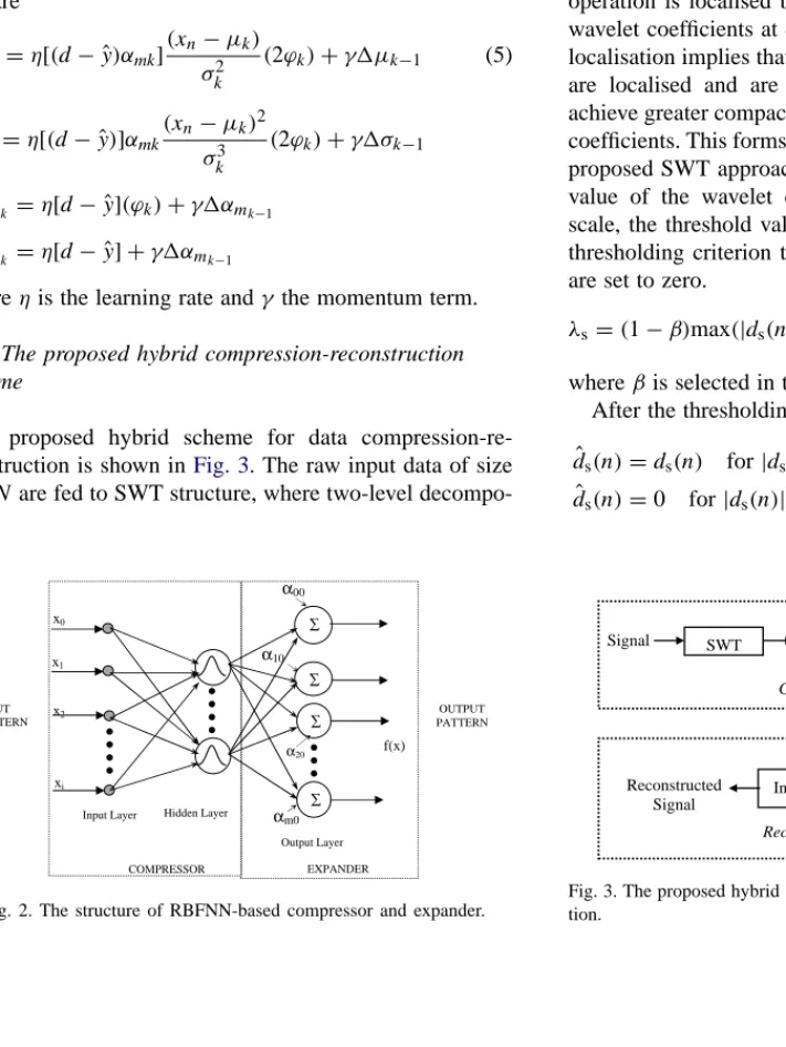
The RBFNN has number of advantages over conventional multi-layered neural network; such as higher accuracy, less training time, simple topology and no local minima problem [13,14].Fig. 2 depicts the detail structure of the RBFNN where the hidden nodes contain the radial basis function. Each hidden unit in the network has two param-eters called a centre (µ), and a width (σ) associated with it. The RBF of the hidden units is radially symmetric in the input space and the output of each hidden unit depends only on the radial distance between the input vector x and the centre parameter µ for the hidden unit. The response of each hidden unit is scaled by its connecting weights (α’s) to the output units and then summed to produce the final network output. The overall network output is therefore ˆ y(n)=f(xn)=αm0+ K k=1 αmkφk(xn) (3)
For each input xn, n represents the time index, K the num-ber of hidden units, αmk the connecting weight of the kth hidden unit to output layer, αm0 the bias term, m is the
number of output.
The value ofφk(xn) is given by
φk(xn)=exp −1 σ2 k xn−µk2 (4)
where µk is the centre vector for the kth hidden unit and
σk is the width of the RBF and || || denotes the Euclidean norm.
In this paper, the parameters of the RBF network are up-dated using the first derivative of the error function with respect to network parameters. With the error vector at the output unit beinge=(d− ˆy), where d is the desired output vector andyˆ the estimated output vector and E1 being half
of the squared error vector, the updating equations for the parameters of the network are derived by taking the partial
HPD 2 LPD 2 LPD 2 HPD 2 LPD 2 HPD 2 THRESHOLDING Compressed data Original PQ event data (a) 2 2 2 2 LPR HPR LPR HPR 2 2 LPR HPR Compressed data Reconstructed PQ event data (b)
Fig. 1. Two level multi-resolution pyramid processing of the PQ event data using DWT and IDWT: (a) decomposition and (b) reconstruction.
derivative of E1. The relevant equations derived for the
train-ing are µk=η[(d− ˆy)αmk] (xn−µk) σ2 k (2ϕk)+γµk−1 (5) σk =η[(d− ˆy)]αmk (xn−µk)2 σ3 k (2ϕk)+γσk−1 αmk =η[d− ˆy](ϕk)+γαmk−1 αmk =η[d− ˆy]+γαmk−1
whereηis the learning rate andγ the momentum term.
2.3. The proposed hybrid compression-reconstruction scheme
A proposed hybrid scheme for data compression-re-construction is shown inFig. 3. The raw input data of size 1×N are fed to SWT structure, where two-level
decompo-∑ ∑ x1 x2 xi Hidden Layer Input Layer Output Layer f(x) α20 α10 ∑ α00 ∑ αm0 COMPRESSOR EXPANDER INPUT PATTERN OUTPUT PATTERN x0
Fig. 2. The structure of RBFNN-based compressor and expander.
sition is accomplished. The wavelet function used in SWT operation is localised both in time and frequency yielding wavelet coefficients at different scales. The time-frequency localisation implies that more energetic wavelet coefficients are localised and are sparse in nature. As a result, we achieve greater compact support from the wavelet transform coefficients. This forms the basis of data compression by the proposed SWT approach. Based on the absolute maximum value of the wavelet coefficients ds(n) at the associated
scale, the threshold value λs is selected and applying hard
thresholding criterion the insignificant wavelet coefficients are set to zero.
λs =(1−β)max(|ds(n)|) (6)
whereβis selected in the range of 0< β <1. After the thresholding,
ˆ ds(n)=ds(n) for|ds(n)| ≥λs ˆ ds(n)=0 for|ds(n)|< λs (7) Signal SWT Thresholding RBFNN Compressor Compression Stage RBFNN Expander Inverse SWT Reconstructed Signal Reconstruction Stage
Fig. 3. The proposed hybrid scheme for data compression and reconstruc-tion.
coefficients is smaller than the original input data P repre-sented byP =1×N. After thresholding operation is per-formed the number of data is reduced to P1. Then the CR by
the SWT method alone is given by CR1=P/P1. In the
pro-cess the energetic SWT coefficients and the original input data are represented by B-bits. In the next stage, we propose a RBFNN to compress the energetic coefficients further. The RBF structure we choose consists of three layers with same number of input and output nodes but less number of hidden nodes. This choice is made to achieve further compression in this encoding stage. It is to be noted that the input and hidden layers are used for compression and the output layer is utilised for expansion purpose. The training of these net-works is carried out using the conventional back propaga-tion (BP) algorithm. The trained RBF network thus formed represents the second stage of compression-reconstruction scheme. Each threshold-coefficient obtained from the first stage is converted into B-bit and is fed to the network and the corresponding reduced number of bit patterns (B1-bit)
available at the hidden node denotes its compact represen-tation. Thus, the RBF network offers a CR given by CR2= B/B1. Hence, the overall CR of the hybrid scheme is CR=
CR1×CR2=(P×B)/(P1×B1).
For training purpose, a given pattern is simultaneously ap-plied both at the input and output of the neural structure and learning is continued until the mean squared error (MSE) attains a possible minimum value. At this stage, learning is discontinued and the corresponding trained network repre-sents a compression-reconstruction network. The portion of the trained network from the input to the hidden nodes per-forms compression operation whereas the remaining portion acts as reconstruction network. The overall reconstruction of the data takes place in the reversed order. Firstly, each of the reduced bit pattern (B1-bit) is applied to the RBF-expander
which reconstructs its original B-bit. Each estimated B-bit pattern represents the corresponding threshold-coefficients. After obtaining threshold coefficients the inverse operation of the SWT is then applied to these data to reconstruct the original input signal.
The overall performance of the complete hybrid scheme is evaluated in terms of MSE (in dB) and PER in the recon-structed are defined as
MSE=10 log10 1 N N i=1 x(i)− ˆx(i)2 (8) PER=
(vector norm of compressed coefficients)2
(vector norm of uncompressed coefficients)2
×100 (9)
The proposed compression scheme is general in nature in the sense that it can be applied to any type of signal. This is because the RBF network is trained with random binary pattern but not with any specific patterns.
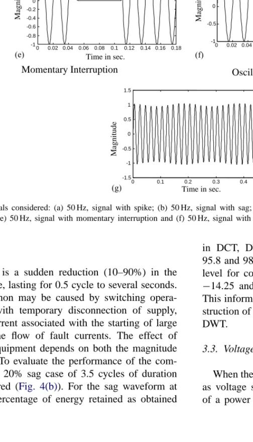
The proposed data compression technique is applied to many PQ issues such as: sag, swell, harmonics, interruption, oscillatory transient and fluctuation shown inFig. 4(a)–(f). All the data are generated using the MATLAB code at a sampling rate of 3 kHz. For neural network trainingη=0.1 andγ=0.04 are considered. To demonstrate the efficacy of the proposed technique some test cases are presented below. For all simulation study a pure sinusoidal signal of 50 Hz and 1 p.u. amplitude is considered. The proposed technique is compared with the standard DCT and DWT (DB-4)-based approaches.
3.1. Voltage spike
A disturbance signal containing a spike for 3 ms dura-tion is considered first. The signal is decomposed by the SWT up to fourth level and the corresponding filter out-puts are shown in Fig. 5. It is evident from these figures that each filter output contains the information of different frequency components of the disturbance signal at differ-ent levels and can accurately localise the disturbance point. Subsequently, a threshold parameter is selected based on the maximum absolute value of the transformed coefficients and then the discarding operation takes place. In the next stage of RBFNN compression, the retained transform coef-ficients are taken into consideration. These compressed data are then utilised to accurately reconstruct the original sig-nal using the reverse operation of the forward process as shown inFig. 3. The reconstructed spike signal depicted in
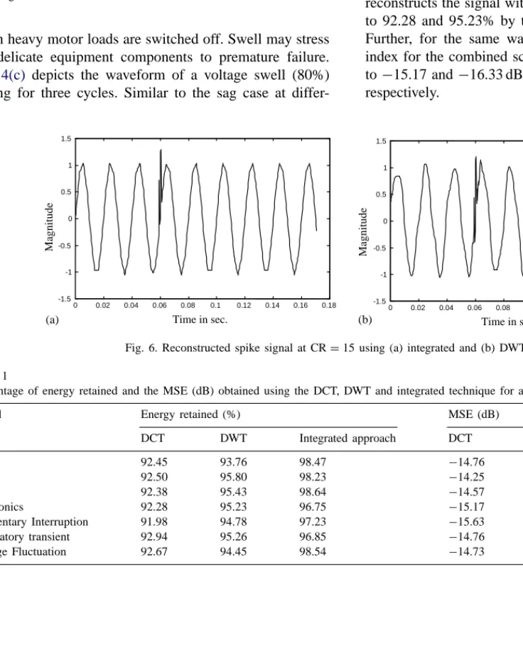
Fig. 6 reveal that the disturbance signal is successfully re-trieved from the transformed coefficients. The ratio between the number of original signal data to the number of data re-tained after the thresholding is termed as the compression ratio (CR) and in the present case CR =15 is considered. With lower CR values, it is observed with simulations that the signal is better retrieved than at CR = 15. It is obvi-ous that with higher CR value less data are retained after thresholding stage and hence accuracy is sacrificed in re-constructing the signal. However, high CR value is preferred for data communication and storage requirements. Further, in case of the combined scheme we have considered signal decomposition up to fourth level with an objective to reduce the computational burden. In practical application, a com-promise is made between these diverging factors.
For spike signal at CR =15, the energy retained by the combined approach is 98.47% as compared to 92.45 and 93.76% by the DCT and DWT approaches, respectively. Similarly, the corresponding MSE for the combined ap-proach is−25.76 dB and that for the DCT and the DWT is
−14.76 and −15.26 dB, respectively. This clearly demon-strates better compression capability of the new technique compared to conventional approaches. In the following dif-ferent PQ signals are considered to see the performance of the new approach.
Oscillatory transient Magnitude Time in sec. 0 0.02 0.04 0.06 0.08 0.1 0.12 0.14 0.16 0.18 0 0.02 0.04 0.06 0.08 0.1 0.12 0.14 0.16 0.18 0 0.02 0.04 0.06 0.08 0.1 0.12 0.14 0.16 0.18 0 0.02 0.04 0.06 0.08 0.1 0.12 0.14 0.16 0.18 -1 -0.8 -0.6 -0.4 -0.2 0 0.2 0.4 0.6 0.8 1 -1 -0.8 -0.6 -0.4 -0.2 0 0.2 0.4 0.6 0.8 1 -1 -0.8 -0.6 -0.4 -0.2 0 0.2 0.4 0.6 0.8 1 0 0.02 0.04 0.06 0.08 0.1 0.12 0.14 0.16 0.18 -1 -0.5 0 0.5 1 1.5 Magnitude Time in sec. Magnitude Time in sec. 0 0.02 0.04 0.06 0.08 0.1 0.12 0.14 0.16 0.18 -2 -1.5 -1 -0.5 0 0.5 1 1.5 2 3rd and 5th harmonics Magnitude Time in sec. Magnitude Time in sec. Momentary Interruption Magnitude Time in sec. -1 -0.5 0 0.5 1 1.5 Magnitude Time in sec. 0 0.1 0.2 0.3 0.4 0.5 -1.5 -1 -0.5 0 0.5 1 1.5 (a) (b) (c) (d) (e) (f) (g)
Fig. 4. Different signals considered: (a) 50 Hz, signal with spike; (b) 50 Hz, signal with sag; (c) 50 Hz, signal with swell; (d) 50 Hz, signal with third and fifth harmonics; (e) 50 Hz, signal with momentary interruption and (f) 50 Hz, signal with oscillatory transient.
3.2. Voltage sag
A voltage sag is a sudden reduction (10–90%) in the voltage magnitude, lasting for 0.5 cycle to several seconds. Such a phenomenon may be caused by switching opera-tion associated with temporary disconnecopera-tion of supply, flow of heavy current associated with the starting of large motor load or the flow of fault currents. The effect of voltage sag on equipment depends on both the magnitude and its duration. To evaluate the performance of the com-bined approach a 20% sag case of 3.5 cycles of duration signal is considered (Fig. 4(b)). For the sag waveform at CR = 15, the percentage of energy retained as obtained
in DCT, DWT and the combined approaches are 92.5, 95.8 and 98.23%, respectively (Table 1). Further, the MSE level for combined scheme is −24.56 dB as compared to
−14.25 and −16.93 dB for DCT and DWT, respectively. This information clearly indicates better accuracy of recon-struction of the proposed scheme over each of the DCT and DWT.
3.3. Voltage swell
When the voltage signal increases by 10–90% it is known as voltage swell. They often appear on the sound phases of a power system where phase-to-ground fault occurs or
-1 0 1 1 st level details -0.2 0 0.2 2 nd level details 0 100 200 300 400 500 -0.5 0 0.5 3 rd level details -2 0 2
Fig. 5. SWT filter bank output at different level of decomposition for spike signal.
when heavy motor loads are switched off. Swell may stress the delicate equipment components to premature failure.
Fig. 4(c) depicts the waveform of a voltage swell (80%) lasting for three cycles. Similar to the sag case at
differ-Magnitude Time in sec. (a) 0 0.02 0.04 0.06 0.08 0.1 0.12 0.14 0.16 0.18 -1.5 -1 -0.5 0 0.5 1 1.5 Magnitude Time in sec. (b) 0 0.02 0.04 0.06 0.08 0.1 0.12 0.14 0.16 0.18 -1.5 -1 -0.5 0 0.5 1 1.5
Fig. 6. Reconstructed spike signal at CR=15 using (a) integrated and (b) DWT scheme. Table 1
Percentage of energy retained and the MSE (dB) obtained using the DCT, DWT and integrated technique for all the PQ events date at CR=15
Signal Energy retained (%) MSE (dB)
DCT DWT Integrated approach DCT DWT Integrated approach
Spike 92.45 93.76 98.47 −14.76 −15.26 −25.76 Sag 92.50 95.80 98.23 −14.25 −16.93 −24.56 Swell 92.38 95.43 98.64 −14.57 −16.87 −22.01 Harmonics 92.28 95.23 96.75 −15.17 −16.33 −23.45 Momentary Interruption 91.98 94.78 97.23 −15.63 −16.89 −25.47 Oscillatory transient 92.94 95.26 96.85 −14.76 −15.63 −24.74 Voltage Fluctuation 92.67 94.45 98.54 −14.73 −16.63 −23.78
scheme show higher accuracy both in terms of energy re-tained and MSE as compared to that of DCT and DWT. For example, at CR = 15, the percentage of energy retained as obtained by the DCT and DWT approaches are 92.38 and 95.43, respectively, as compared to 98.64 by the new approach (Table 1). Further, the MSE for the waveform in case of new scheme is as low as −22.01 dB as com-pared to −14.57 and −16.87 dB for the DCT and DWT, respectively. In the case of voltage swell also, superior per-formance of the combined scheme of data compression is observed.
3.4. Harmonically distorted signal
With the introduction of more power electronic equip-ments in distribution system, the power quality is further degraded as they produce significant amount of different harmonics. Such harmonic pollution in voltage signal leads to poor performance of converter circuit. A fundamental voltage signal (50 Hz) of 1 p.u. distorted by 30% third har-monic and 10% fifth harhar-monic (Fig. 4(d)) is considered to evaluate the performance of the combined data com-pression technique. AT CR = 15, the proposed scheme reconstructs the signal with 96.75% of energy as compared to 92.28 and 95.23% by the DCT and DWT, respectively. Further, for the same waveform and CR value the MSE index for the combined scheme is−23.45 dB as compared to−15.17 and−16.33 dB obtained by the DCT and DWT, respectively.
3.5. Momentary interruption
Interruptions can be considered as voltage sags with 100% amplitude and are mainly due to short circuit faults being cleared by the protection. Supply interruption for few cycles will greatly influence the performance of glass and computer industries. For evaluating the performance of the combined data compression technique a voltage signal interrupted for three cycles as shown in Fig. 4(e)is considered. The new scheme reconstructs the signal with 97.23% of energy (91.98 and 94.78% for the DCT and DWT, respectively). Sim-ilarly, the MSE for the combined scheme is −25.47 dB as compared to −15.63 and −16.89 dB for the DCT and DWT, respectively. This simulation study is extended to other CR values and it is, general, found that the combined scheme is a better candidate for data compression of such signals.
3.6. Oscillatory transient
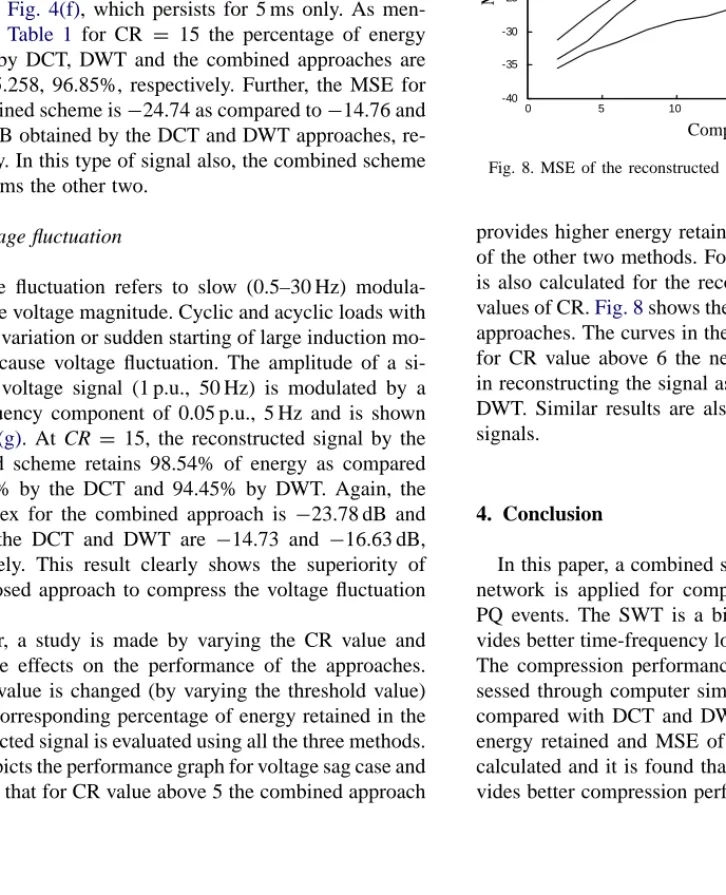
Transient disturbances are shorter than the sags and swells. A transient disturbance waveform may have os-cillatory characteristic and such signals are found during capacitor bank switching. An oscillatory transient signal is shown in Fig. 4(f), which persists for 5 ms only. As men-tioned in Table 1 for CR = 15 the percentage of energy retained by DCT, DWT and the combined approaches are 92.94, 95.258, 96.85%, respectively. Further, the MSE for the combined scheme is−24.74 as compared to−14.76 and
−15.63 dB obtained by the DCT and DWT approaches, re-spectively. In this type of signal also, the combined scheme outperforms the other two.
3.7. Voltage fluctuation
Voltage fluctuation refers to slow (0.5–30 Hz) modula-tion of the voltage magnitude. Cyclic and acyclic loads with temporal variation or sudden starting of large induction mo-tors can cause voltage fluctuation. The amplitude of a si-nusoidal voltage signal (1 p.u., 50 Hz) is modulated by a low-frequency component of 0.05 p.u., 5 Hz and is shown in Fig. 4(g). At CR = 15, the reconstructed signal by the combined scheme retains 98.54% of energy as compared to 92.67% by the DCT and 94.45% by DWT. Again, the MSE index for the combined approach is −23.78 dB and that for the DCT and DWT are −14.73 and −16.63 dB, respectively. This result clearly shows the superiority of the proposed approach to compress the voltage fluctuation signal.
Further, a study is made by varying the CR value and to see the effects on the performance of the approaches. The CR value is changed (by varying the threshold value) and the corresponding percentage of energy retained in the reconstructed signal is evaluated using all the three methods.
Fig. 7depicts the performance graph for voltage sag case and it is clear that for CR value above 5 the combined approach
0 5 10 15 20 25 30 70 75 80 85 90 95 100 Compression ratio
Percentage of energy retained
a b c a− Proposed method b− DWT c− DCT
Fig. 7. Percentage of energy retained in the reconstructed sag signal using different methods. 0 5 10 15 20 25 30 -40 -35 -30 -25 -20 -15 -10 -5 0 Compression ratio MSE in dB a b c a− Proposed method b− DWT c− DCT
Fig. 8. MSE of the reconstructed sag signal using different methods.
provides higher energy retaining capacity compared to that of the other two methods. For the same sag case, the MSE is also calculated for the reconstructed signal for different values of CR.Fig. 8shows the MSE as obtained by different approaches. The curves in the two figures clearly show that for CR value above 6 the new approach is more accurate in reconstructing the signal as compared to the DCT or the DWT. Similar results are also obtained for other types of signals.
4. Conclusion
In this paper, a combined scheme using SWT and neural network is applied for compression of data pertaining to PQ events. The SWT is a bi-orthogonal wavelet and pro-vides better time-frequency localisation than DCT or DWT. The compression performance of the new approach is as-sessed through computer simulations where the results are compared with DCT and DWT approaches. Percentage of energy retained and MSE of reconstructed PQ signals are calculated and it is found that the integrated approach pro-vides better compression performance than DCT or DWT.
[1] J. Arrillaga, M.H.J. Bollen, N.R. Watson, Power quality following deregulation, IEEE Proc. 88 (2) (2000) 246–261.
[2] K.R. Rao, P. Yip, Discrete Cosine Transform: Algorithms, Advan-tages, and Applications, Academic Press, New York, 1990. [3] S. Santoso, et al., Power quality assessment via wavelet
trans-form analysis, IEEE Trans. Power Delivery 11 (1995) 924– 930.
[4] L. Angrisani, et al., A measurement method based on the wavelet transform for power quality analysis, IEEE Trans. Power Delivery, No. PE-056-PWRD-0-1-1998.
[5] S. Santoso, E.J. Power, W.M. Grady, Power quality disturbance data compression using wavelet transform methods, IEEE Trans. Power Delivery 12 (3) (1997) 1250–1256.
[6] T.B. Littler, D.J. Morrow, Wavelets for analysis and compression of power system disturbances, IEEE Trans. Power Delivery 14 (2) (1999) 358–364.
[7] G. Strange, T. Nguyen, Wavelets and Filterbanks, Wellesley-Cambridge, Wellesley, MA, 1996.
hierarchical neural network, IEEE Trans. Aerospace Electron. Syst. 32 (1) (1996) 326–338.
[9] M. Unser, Splines: A perfect fit for signal and image processing, IEEE Signal Process. Mag., November 1999.
[10] A. Cohen, I. Daubechies, J.C. Feauveau, Bi-orthogonal bases of compactly supported wavelets, Comm. Pure Appl. Math. 45 (1992) 485–560.
[11] C.K. Chui, J.Z. Wang, On compactly supported spline wavelets and a duality principle, Trans. Am. Math. Soc. 330 (2) (1992) 903–915. [12] P.K. Dash, B.K. Panigrahi, D.K. Sahoo, G. Panda, Power quality disturbance data compression, detection, and classification using in-tegrated spline wavelet and S-transform, IEEE Trans. Power Delivery 18 (2) (2003) 595–600.
[13] L. Yingwei, N. Sundarrajan, P. Saratchandran, Performance evalua-tion of a sequential minimal radial basis funcevalua-tion (RBF) neural net-work learning algorithm, IEEE Trans. Neural Netnet-works 9 (2) (1998) 308–318.
[14] L. Tarassenko, S. Roberts, Supervised and unsupervised learning in radial basis function classifiers, IEE Proc. Vis. Image Signal Process. 141 (4) (1994) 210–216.