Efficient Processing of Window Functions in Analytical SQL Queries

(1)

Efficient Processing of Window Functions

in Analytical SQL Queries

Viktor Leis

Technische Universit ¨at M ¨unchen

Kan Kundhikanjana

Alfons Kemper

Thomas Neumann

ABSTRACT

Window functions, also known as analytic OLAP functions, have been part of the SQL standard for more than a decade and are now a widely-used feature. Window functions allow to elegantly express many useful query types including time series analysis, ranking, percentiles, moving averages, and cumulative sums. Formulating such queries in plain SQL-92 is usually both cumbersome and in-efficient.

Despite being supported by all major database systems, there have been few publications that describe how to implement an effi-cient relational window operator. This work aims at filling this gap by presenting an efficient and general algorithm for the window operator. Our algorithm is optimized for high-performance main-memory database systems and has excellent performance on mod-ern multi-core CPUs. We show how to fully parallelize all phases of the operator in order to effectively scale for arbitrary input dis-tributions.

1. INTRODUCTION

Window functions, which are also known as analytic OLAP functions, are part of the SQL:2003 standard. This SQL feature is widely used—the TPC-DS benchmark [18], for example, uses window functions in 9 out of 99 queries. Almost all major database systems, including Oracle [1], Microsoft SQL Server [2], IBM DB2 [3], SAP HANA [4], PostgreSQL [5], Actian VectorWise [14], Cloudera Impala [16], and MonetDB [6] implement the functional-ity described in the SQL standard—or at least some subset thereof. Window functions allow to easily formulate certain business in-telligence queries that include time series analysis, ranking, top-k, percentiles, moving averages, cumulative sums, etc. Without win-dow function support, such queries either require difficult to formu-late and inefficient correformu-lated subqueries, or must be implemented at the application level.

The following example query, which might be used to detect out-liers in a time series, illustrates the use of window functions in SQL. This work is licensed under the Creative Commons Attribution-NonCommercial-NoDerivs 3.0 Unported License. To view a copy of this li-cense, visit http://creativecommons.org/licenses/by-nc-nd/3.0/. Obtain per-mission prior to any use beyond those covered by the license. Contact copyright holder by emailing [email protected]. Articles from this volume were invited to present their results at the 41st International Conference on Very Large Data Bases, August 31st - September 4th 2015, Kohala Coast, Hawaii.

select location, time, value, abs(value-(avg(value) over w))/(stddev(value) over w)

from measurement

window w as (

partition by location

order by time

range between 5 preceding and 5 following)

The query normalizes each measurement by subtracting the aver-age and dividing by the standard deviation. Both aggregates are computed over a window of 5 time units around the time of the measurement and at the same location. Without window functions, it is possible to state the query as follows:

select location, time, value, abs(value-(select avg(value)

from measurement m2

where m2.time between m.time-5 and m.time+5

and m.location = m2.location)) / (select stddev(value)

from measurement m3

where m3.time between m.time-5 and m.time+5

and m.location = m3.location)

from measurement m

In this formulation, correlated subqueries are used to compute the aggregates, which in most query processing engines results in very slow execution times due to quadratic complexity. The exam-ple also illustrates that to imexam-plement window functions efficiently, a new relational operator is required. Window expressions cannot be replaced by simple aggregation (i.e.,group by) because each measurement defines a separate window. More examples of useful window function queries can be found in Appendix A.

Despite the usefulness and prevalence of window functions “in the wild”, the window operator has mostly been neglected in the literature. One exception is the pioneering paper by Cao et al. [12], which shows how to optimizemultiplewindow functions that occur in one queryby avoiding unnecessary sorting or partitioning steps. In this work, we instead focus on the core algorithm for efficient window function computation itself. The optimization techniques from [12] are therefore orthogonal and should be used in conjunc-tion.

To the best of our knowledge, we present the first detailed de-scription of a complete algorithm for the window operator. Our al-gorithm is universally applicable, efficient in practice, and asymp-totically superior to algorithms currently employed by commercial systems. This is achieved by utilizing a specialized data structure, the Segment Tree, for window function evaluation. The design

(2)

of the window operator is optimized for high-performance main-memory databases like our HyPer [15] system, which is optimized for modern multi-core CPUs [17]

As commodity server CPUs with dozens of cores are becoming widespread, it becomes more and more important to parallelizeall operations that depend on the size of the input data. Therefore, our algorithm is designed to be highly scalable: instead of only support-ing inter-partition parallelism, which is a best-effort approach that is simple to implement but not applicable to all queries, we show how to parallelizeallphases of our algorithm. At the same time, we opportunistically use low-overhead, partitioning-based paralleliza-tion when possible. As a result, our implementaparalleliza-tion is fast and scales even for queries without a partitioning clause and for arbi-trary, even highly skewed, input distributions.

The rest of the paper is organized as follows: Section 2 gives an overview of the syntax and semantics of window functions in SQL. The core of our window operator and our parallelization strategy is presented in Section 3. The actual computation of window function expressions, which is the last phase of our operator, is discussed in Section 4. In Section 5 we experimentally evaluate our algorithm under a wide range of settings and compare it with other imple-mentations. Finally, after presenting related work in Section 6, we summarize the paper and discuss future research in Section 7.

2. WINDOW FUNCTIONS IN SQL

One of the core principles of SQL is that the output tuple order of all operators (except for sort) is undefined. This design decision en-ables many important optimizations, but makes queries that depend on the tuple order (e.g., ranking) or that refer to neighboring tuples (e.g., cumulative sums) quite difficult to state. By allowing to refer to neighboring tuples (the “window”) directly, window functions allow to easily express such queries.

In this section, we introduce the syntax and semantics of SQL window functions. To understand the semantics two observations are important. Firstly, window function expressions are computed after most other clauses (including group by and having), but before the final sorting order by and duplicate removal

distinctclauses. Secondly, the window operator only com-putes additional attributes for each input tuple but does not change or filter its input otherwise. Therefore, window expressions are only allowed in theselectandorder byclauses, but not in thewhereclause.

2.1 Partitioning

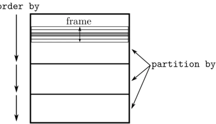
Window function evaluation is based on three simple and orthog-onal concepts: partitioning, ordering, and framing. Figure 1 il-lustrates these concepts graphically. Thepartition byclause partitions the input by one or more expressions into independent groups, and thereby restricts the window of a tuple. In contrast to normal aggregation (group by), the window operator does not reduce all tuples of a group to a single tuple, but only logically par-titions tuples into groups. If no partitioning clause is specified, all input rows are considered as belonging to the same partition.

2.2 Ordering

Within each partition, the rows can be ordered using theorder byclause. Semantically, theorder byclause defines how the input tuples are logically ordered during window function evalua-tion. For example, if a ranking window function is used, the rank is computed with respect to the specified order. Note that the or-dering only affects window function processing but not necessarily the final order of the result. If no ordering is specified, the result of some window functions (e.g.,row number) is non-deterministic.

order by

partition by

frame

Figure 1: Window function concepts: partitioning, ordering, framing. The current (gray) row can access rows in its frame. The frame of a tuple can only encompass tuples from that par-tition

order by

2.5 4 5 6 7.58.5 10 12

range between 3 preceding and 3 following

rows between 3 preceding and 3 following

Figure 2: Illustration of therangeandrowsmodes for fram-ing. Each tick represents the value of a tuple’sorder by ex-pression

2.3 Framing

Besides the partitioning clause, window functions have aframing clausewhich allows to restrict the tuples that a window function acts on further. The frame specifies which tuples in the proximity of the current row (based on the specified ordering) belong to its frame. Figure 2 illustrates the two available modes.

• rowsmode directly specifies how many rows before or after the current row belong to the frame. In the figure, the 3 rows before and after the current row are part of the frame, which also includes the current row therefore consists of the values 4,5,6, 7.5, 8.5, 10, and12. It is also possible to specify a frame that does not include the current row, e.g., rows between 5 preceding and 2 preceding. • Inrangemode, the frame bounds are computed by

decre-menting/incrementing theorder byexpression of the cur-rent row1. In the figure, theorder byexpression of the current row is7.5, the window frame bounds are4.5(7.5−3) and10.5(7.5−3). Therefore, the frame consists of the val-ues5,6,7.5,8.5, and10.

In both modes, the framing bounds do not have to be constants, but can be arbitrary expressions and may even depend on attributes of the current row. Most implementations only support constant values for framing bounds, whereas our implementation supports non-constant framing bounds efficiently. All rows in the same par-tition that have the sameorder byexpression values are consid-eredpeers. The peer concept is only used by some window func-tions, but ignored by others. For example, all peers have the same

rank()but a differentrow number().

1_range_{mode is only possible if the query has exactly one numeric} order by expression.

(3)

Besidesprecedingandfollowing, the frame bounds can also be set to the following values:

• current row: the current row (including all peers in

rangemode)

• unbounded preceding: the frame starts at the first row in the partition

• unbounded following: the frame ends with the last row in the partition

If no window frame was specified and there is an order byclause, the default frame specification isrange between unbounded preceding and current row. This results in a window frame that consists of all rows from the start of the current partition to the current row and all its peers, and is useful for computing cumulative sums. Queries without an

order byclause, are evaluated over the entire partition, as if having the frame specificationrange between unbounded preceding and unbounded following. Finally, it is important to note that the framing clause only affects some window functions, namely intra-window navigation functions (first value, last value, nth value), and non-distinct aggregate functions (min,max,count,sum,avg). The remain-ing window functions (row number,rank,lead, . . . ) and dis-tinct aggregates are always evaluated on the entire partition.

For syntactic convenience and as already shown in the first ex-ample of the introduction, SQL allows to name a particular combi-nation of partitioning, ordering, and framing clauses. By referring to this name the window specification can then be reused by multi-ple window expressions to avoid repeating the clauses, which often improves the readability of the query, as shown in the following example:

select min(value) over w1, max(value) over w1, min(value) over w2, max(value) over w2

window

w1 as (order by time

range between 5 preceding and 5 following), w2 as (order by time

range between 3 preceding and 3 following)

2.4 Window Expressions

SQL:2011 defines a number of window functions for different purposes. The following functions ignore framing, i.e., they are always evaluated on the entire partition:

• ranking:

– rank(): rank of the current row with gaps

– dense rank(): rank of the current row without gaps – row number(): row number of the current row – ntile(num): distribute evenly over buckets (returns

integer from 1 tonum) • distribution:

– percent rank(): relative rank of the current row – cume dist(): relative rank of peer group • navigation in partition:

– lead(expr, offset, default): evaluate

expron preceding row in partition

– lag(expr, offset, default): evaluate

expron following row in partition

• distinct aggregates: min, max,sum, . . . : compute distinct aggregate over partition

There are also window functions that are evaluated on the current frame, i.e., a subset of the partition:

• navigation in frame:

– first expr(expr), last expr(expr),

nth expr(expr, nth): evaluate expr on first/last/nthrow of the frame

• aggregates:min,max,sum, . . . : compute aggregate over all tuples in the current frame

As the argument lists of these functions indicate, most functions require an arbitrary expression (theexprargument) and other ad-ditional parameters as input.

To syntactically distinguish normal aggregation functions (com-puted by the group by operator) from their window function cousins, which have the same name but are computed by the aggre-gation operator, window function expressions must be followed by theoverkeyword and a (potentially empty) window frame speci-fication. In the following query, the average is computed using the window operator, whereas the sum aggregate is computed by the aggregation operator:

select cid, year, month, sum(price),

avg(sum(price)) over (partition by cid)

from orders

group by customer_id, year, month

For each customer and month, the query computes the sum of all purchases of this customer (using aggregation) and the average of all monthly expenditures of this customer (using window aggrega-tion without framing).

3. THE WINDOW OPERATOR

Depending on the window function and the partitioning, order-ing, and framing clause specified (or omitted) in a particular query, the necessary algorithmic steps differ greatly. In order to incorpo-rate all aspects into a single operator we present our algorithm in a modular fashion. Some phases can simply be omitted if they are not needed for a particular query.

The basic algorithm for window function processing directly fol-lows from the high-level syntactic structure discussed in Section 2 and involves the following phases:

1. Partitioning: partition the input relation using thepartition byattributes

2. Sorting: sort each partition using theorder byattributes 3. Window function computation: for each tuple

(a) Compute window frame: Determine window frame (a subset of the partition)

(b) Evaluate window function: Evaluate window function on the window frame

In this section we focus on the first two phases, partitioning and sorting. Phase 3, window function evaluation, is discussed in Sec-tion 4.

(4)

hash partitioning (thread-local)

thread 1 thread 2

combine hash groups

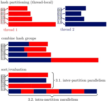
3.1. inter-partition parallelism 3.2. intra-partition parallelism sort/evaluation 00 01 10 11 00 01 10 11 00 01 10 11 00 01 10 11

Figure 3: Overview of the phases of the window operator. The colors represent the two threads

3.1 Partitioning and Sorting

For the initial partitioning and sorting phases there are two tradi-tional methods:

1. The hash-based approach fully partitions the input using hash values of the partition byattributes before sort-ing each partition independently ussort-ing only theorder by

attributes.

2. Thesort-based approach first sorts the input by both the

partition byand theorder byattributes. The parti-tion boundaries are determined “on-the-fly” during the win-dow function evaluation phase (phase 3), e.g., using binary search.

From a purely theoretical point of view, the hash-based approach is preferable. Assuming there aren input rows andO(n) parti-tions, the overall complexity of the hash-based approach isO(n), whereas the sort-based approach results inO(nlogn)complexity. Nevertheless, thesort-basedapproach is often used in commercial systems—perhaps because it requires less implementation effort, as a sorting phase is always required anyway. In order to achieve good performanceandscalability we use combination of both methods.

In single-threaded execution, it is usually best to first fully par-tition the input data using a hash table. With parallel execution, a concurrent hash table would be required for this approach. We have found, however, that concurrent, dynamically-growing hash tables (e.g., split-ordered lists [23]) have a significant overhead in comparison with unsynchronized hash tables. The sort-based ap-proach, without partitioning first, is also very expensive. There-fore, to achieve high scalability and low overhead, we use a hybrid approach that combines the two methods.

3.2 Pre-Partitioning into Hash Groups

Our approach is to partition the input data into a constant number (e.g., 1024) ofhash groups, regardless of how many partitions the input data has. The number of hash groups should be a power of 2

and larger than the number of threads but small enough to make par-titioning efficient on modern CPUs. This form of parpar-titioning can be done very efficiently in parallel due to limited synchronization requirements: As illustrated in Figure 3, each thread (distinguished using different colors) initially has its own array of hash groups (4 in the figure)2. After all threads have partitioned their input data, the corresponding hash groups from all threads are copied into a combined array. This can be done in parallel and without synchro-nization because at this point the sizes and offsets of all threads’ hash groups are known. After copying, each combined hash group is stored in a contiguous array, which allows for efficient random access to each tuple.

After the hash groups copied, the next step is to sort them by both the partitioning and the ordering expressions. As a result, all tuples with the same partitioning key are adjacent in the same hash group, although of course a hash group may contain multiple partitioning keys. When necessary, the actual partition boundaries can be de-termined using binary search as in the sort-based approach during execution of the remaining window function evaluation step.

3.3 Inter- and Intra-Partition Parallelism

At first glance, the window operator seems to be embarrass-ingly parallel, as partitioning can be done in parallel and all hash groups are independent from each other: Since sorting and window function evaluation for different hash groups is independent, the available threads can simply work on different hash groups with-out needing any synchronization. Database systems that parallelize window functions usually use this strategy, as it is easy to im-plement and can offer very good performance for “good-natured” queries.

However, this approach is not sufficient for queries with no parti-tioning clause, when the number of partitions is much smaller than the number of threads, or if the partition sizes are heavily skewed (i.e., one partition has a large fraction of all tuples). Therefore, to fully utilize modern multi- and many-core CPUs, which often have dozens of cores, the simple inter-partitionparallelism approach alone is not sufficient. For some queries, it is additionally neces-sary to supportintra-partitionparallelism, i.e., to parallelize within hash groups.

We use intra-partition parallelism only for large hash groups. When there are enough hash groups for the desired number of threads and none of these hash groups is too large, inter-partition parallelism is sufficient and most efficient. Since the sizes of all hash groups are known after the partitioning phase, we can dy-namically assign each hash group into either the inter- or the intra-partition parallelism class. This classification takes the size of the hash group, the total amount of work, and the number of threads into account. In Figure 3, intra-partition parallelism is only used for hash group 11, whereas the other hash groups use inter-partition parallelism. Our approach is resistant to skew and always utilizes the available hardware parallelism while exploiting low-overhead inter-partition parallelism when possible.

When intra-partition parallelism is used, a parallel sorting algo-rithm must be used. Additionally, the window function evaluation phase itself must be parallelized, as we describe in the next section.

2

In our implementation in HyPer, the thread-local hash groups physically consist of multiple, chained arrays, since no random ac-cess is neac-cessary and the chunks are copied into a combined ar-ray anyway. Furthermore, all types conceptually have a fixed size (variable-length types like strings are stored as pointers), which al-lows the partitioning and sorting phases to work on the tuples di-rectly instead of pointers.

(5)

4. WINDOW FUNCTION EVALUATION

As mentioned before, some window functions are affected by framing and some ignore it. Consequently, their implementations are quite different and we discuss them separately. We start with those window functions that are affected by framing.

4.1 Basic Algorithmic Structure

After the partitioning and sorting phases, all tuples that have the same partitioning key are stored adjacently, and the tuples are sorted by theorder byexpressions. Based on this representa-tion, window function evaluation can be performed in parallel by assigning different threads to different subranges of the hash group. In single-threaded execution or with inter-partition parallelism the entire hash group is assigned to one thread.

To compute a window function, the following steps are necessary for each tuple:

1. determine partition boundaries 2. determine window frame

3. compute window function over the frame and output tuple The first step, computing the partition boundaries, is necessary be-cause a hash group can contain multiple (logical) partitions, and is done using binary search. The two remaining steps, determining the window frame bounds and window function evaluation, which is the main algorithmic challenge, are discussed in the following two sections. Pseudo code for this basic code structure can be found in Appendix B.

4.2 Determining the Window Frame Bounds

For window functions that are affected by framing, for each tu-ple it is necessary to determine the indexes of the window frame bounds. Since we store the tuples in arrays, the tuples in the frame can then easily be accessed. The implementation ofrowsmode is obvious and fast; one simply needs to add/subtract the index of the current row to the bounds while ensuring that the bounds remain in the current partition.

rangemode is slightly more complicated. If the bounds are constant, one can keep track of the previous window and advance the start and end window one-by-one as needed3. It is clear that the frame start only advances by at mostnrows in total (and anal-ogously for the frame end). Therefore, the complexity for finding the frame forntuples isO(n). If, inrangemode, the bounds are not constant, the window can grow and shrink arbitrarily. For this case, the solution is to first add/subtract the bounds from the current ordering key, and then to use binary search which results in a complexity ofO(nlogn). The complexity of computing the window frame fornrows can be summarized as follows:

mode constant non-constant

rows O(n) O(n)

range O(n) O(nlogn)

4.3 Aggregation Algorithms

Once the window frame bounds have been computed for a par-ticular tuple, the final step is to evaluate the desired window func-tion on that frame. For the navigafunc-tion funcfunc-tionsfirst expr,

last expr, andnth exprthis evaluation is simple and cheap 3_{Note that the incremental approach may lead to redundant work} during intra-partition parallelism and with large frame sizes. Thus, to achieve better scalability with intra-partition parallelism, binary search should be employed even for constant frame bounds.

(O(1)), because these functions merely select one row in the win-dow and evaluate an expression on it. Aggregate functions, in con-trast, need to be (conceptually) evaluatedover allrows of the cur-rent window, which makes them more expensive. Therefore, we present and analyze 4 algorithms with different performance char-acteristics for computing aggregates over window frames.

4.3.1 Na¨ıve Aggregation

The na¨ıve approach is to simply loop over all tuples in the window frame and compute the aggregate. The inher-ent problem of this algorithm is that it often performs redun-dant work, resulting in quadratic runtime. In a running-sum query like sum(b) over (order by a rows between unbounded preceding and current row), for exam-ple, for each row of the input relation all values from the first to the current row are added—each time starting anew from the first row, and doing the same work all over again.

4.3.2 Cumulative Aggregation

The running-sum query suggests an improved algorithm, which tries to avoid redundant work instead of recomputing the aggregate from scratch for each tuple. The cumulative algorithm keeps track of the previous aggregation result and previous frame bounds. As long as the window grows (or does not change), only the additional rows are aggregated using the previous result. This algorithm is used by PostgreSQL and works well for some frequently occurring queries, e.g., the default framing specification (range between unbounded preceding and current row).

However, this approach only works well as long as the win-dow frame grows. For queries where the winwin-dow frame can both grow and shrink (e.g., sum(b) over (order by a rows between 5 preceding and 5 following)), one can still get quadratic runtime, because the previous aggregate must be discarded every time.

4.3.3 Removable Cumulative Aggregation

The removable cumulative algorithm, which is used by some commercial database systems, is a further algorithmic refinement. Instead of only allowing the frame to grow before recomputing the aggregate, it permits removal of rows from the previous aggregate. For thesum, count, andavgaggregates, removing rows from the current aggregate can easily be achieved by subtracting. For theminandmaxaggregates, it is necessary to maintain an ordered search tree of all entries in the previous window. For each tuple this data structure is updated by adding and removing entries as neces-sary, which makes these aggregates significantly more expensive.

The removable cumulative approach works well for many queries, in particular for sum and avg window expres-sions, which are more common than min or max in window expressions. However, queries with non-constant frame bounds (e.g., sum(b) over (order by a rows between x preceding and y following)) can be a problem: In the worst case, the frame bounds vary very strongly between neighboring tuples, such that the runtime becomesO(n2).

4.3.4 Segment Tree Aggregation

As we saw in the previous section, even the removable cumu-lative algorithm can result in quadratic execution time because caching the result of the previous window does not help when the window frame changes arbitrarily for each tuple. We therefore in-troduce an additional data structure, the Segment Tree, which al-lows to evaluate an aggregate over an arbitrary frame inO(logn). The Segment Tree stores aggregates for sub ranges of the entire

(6)

0 1 2 3 level 0: sorted tuples

(attributes a,b) 0-3 4-7 0-7 6 7 A,5 B,7 C,3 D,10 F,6 U,2 V,8 W,4 4 5 25 20 45 _{level 1} level 2

Figure 4: Physical Segment Tree representation with fanout 4 for sum(b) over (order by a)

5

7

3

10

6

2

12

13

8

25

45

12

8

4

20

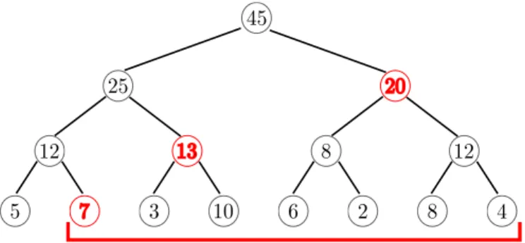
Figure 5: Segment Tree forsumaggregation. Only the red nodes (7, 13, 20) have to be aggregated to compute the sum of 7, 3, 10, 6, 2, 8, 4

hash group, as shown in Figure 5. In the figuresum is used as the aggregate, thus the root node stores the sum of all leaf nodes. The two children of the root store the sums for two equi-width sub ranges, and so on. The Segment Tree allows to compute the ag-gregate over an arbitrary range in logarithmic time by using the associativity of aggregates. For example, to compute the sum for the last 7 values of the sequence, we need to compute the sum of the red nodes 7, 13, and 20.

For illustration purposes, Figure 5 shows the Segment Tree as a binary tree with pointers. In fact, our implementation stores all nodes of each tree level in an array and without any pointers, as shown in Figure 4. In this compact representation, which is similar to that of a standard binary heap, the tree structure is implicit and the child and parent of a node can be determined using arithmetic operations. Furthermore, to save even more space, the lowest level of the tree is the sorted input data itself, and we use a larger fanout (4 in the figure). These optimizations make the additional space consumption for the Segment Tree negligible. Additionally, the higher fanout improves performance, as we show in an experiment that is described in Section 5.7.

In order to compute an aggregate for a given range, the Seg-ment Tree is traversed bottom up starting fromboth window frame bounds. Both traversals are done simultaneously until the traversals arrive at the same node. As a result, this procedure stops early for small ranges and always aggregates the minimum number of nodes. The details of the traversal algorithm can be found in Appendix C. In addition to improving worst-case efficiency, another important benefit of the Segment Tree is that it allows to parallelize arbitrary aggregates, even for running sum queries likesum(b) over (order by a rows between unbounded preceding and current row). This is par-ticularly important for queries without a partitioning clause, which can only use intra-partition parallelism to avoid executing this phase of the algorithm serially. The Segment Tree itself can eas-ily be constructed in parallel and without any synchronization, in

a bottom-up fashion: All available threads scan adjacent ranges of the same Segment Tree level (e.g., using aparallel for con-struct) and store the computed aggregates into the level above it.

For aggregate functions likemin,max,count, andsum, the Segment Tree uses the obvious corresponding aggregate function. For derived aggregate functions likeavgorstddev, it is more ef-ficient to store all needed values (e.g., the sum and the count) in the same Segment Tree instead of having two such trees. Interestingly, besides for computing aggregates, the Segment Tree is also use-ful for parallelizing thedense rankfunction, which computes a rank without gaps. To compute thedense rankof a particular tuple, the number of distinct values that precede this tuple must be known. A Segment Tree where each segment counts the number of distinct child values is easy to construct4, and allows threads to work in parallel on different ranges of the partition.

4.3.5 Algorithm Choice

Table 1 summarizes the worst-case complexities of the 4 algorithms. The na¨ıve algorithm results in quadratic run-time for many common window function queries. The cu-mulative algorithm works well as long as the window frame only grows. Additionally, queries with frames like current row and unbounded followingor1 preceding and unbounded followingcan also be executed efficiently using the cumulative algorithm by first reversing the sort order. The re-movable algorithm further expands the set of queries that can be executed efficiently, but requires an additional ordered tree struc-ture forminandmaxaggregates and can still result in quadratic runtime if the frame bounds are not constant.

Therefore, the analysis might suggest that the Segment Tree al-gorithm should always be chosen, as it avoids quadratic runtime in all cases. However, for many simple queries likerows between 1 preceding and current row, the simpler algorithms perform better in practice because the Segment Tree can incur a significant overhead both for constructing and traversing the tree structure. Intuitively, the Segment Tree approach is only beneficial if the frame frequently changes by a large amount in comparison with the previous tuple’s frame. Unfortunately, in many cases, the optimal algorithm cannot be chosen based on the query structure alone, because the data distribution determines whether building a Segment Tree will pay off. Furthermore, choosing the optimal algorithm becomes even more difficult when one also considers parallelism, because, as mentioned before, the Segment Tree al-gorithmalwaysscales well in the intra-partition parallelism case whereas the other algorithms do not.

Fortunately, we have found that the majority of the overall query time is spent in the partitioning and sorting phases (cf. Figure 2 and

4

Each node of the Segment Tree fordense rankstores the num-ber of distinct values for its segment. To combine two adjacent seg-ments, one simply needs to add their distinct value counts and sub-tract 1 if the neighboring tuples are equal. Note that the Segment Tree is only used for computing the first result (cf. Appendix D).

(7)

rows between ... Na¨ıve Cumulative Removable Cumulative Segment Tree

1 preceding and current row O(n) O(n) O(n) O(nlogn)

unbounded preceding and current row O(n2) O(n) sum:O(n),min:O(nlogn) O(nlogn)

CONST preceding and CONST following O(n2) O(n2) sum:O(n),min:O(nlogn) O(nlogn)

VAR preceding and VAR following O(n2₎ _O₍_n2₎ _sum_:_O₍_n2₎_,_min_:_O₍_n2_log_n₎ _O₍_n_log_n₎ Table 1: Worst-case complexity of computing aggregates forntuples

1 //rank of the current row with gaps 2 rank(begin, end)

3 pBegin = findPartitionBegin(0, begin+1) 4 pEnd = findPartitionEnd(begin)

5 p=findFirstPeer(pBegin,begin)-pBegin+1 6 result[begin] = p

7 for (pos from begin+1 below end) 8 if (pos = pEnd) 9 pBegin = pos 10 pEnd = findPartitionEnd(pos) 11 if (isPeer(pos, pos-1)) 12 result[pos] = result[pos-1] 13 else 14 result[pos] = pos-pBegin+1

Figure 6: Pseudo code for therank function, which ignores framing

Figure 10), thus erring on the side of the Segment Tree is always a safe choice. We therefore propose an opportunistic approach: A simple algorithm like cumulative aggregation is only chosen when there is no risk ofO(n2₎_runtime

andno risk of insufficient par-allelism. This method only uses the static query structure, and does not rely on cardinality estimates from the query optimizer. A query likesum(b) over (order by a rows between unbounded preceding and current row), for exam-ple, can always safely and efficiently be evaluated using the cumu-lative algorithm. Additionally, we choose the algorithm for inter-partition parallelism and the intra-inter-partition parallelism hash groups separately. For example, the small hash groups of a query might use the cumulative algorithm, whereas the large hash groups might be evaluated using the Segment Tree to make sure evaluation scales well. This approach always avoids quadratic runtime, scales well on systems with many cores, while achieving optimal performance for many common queries.

4.4 Window Functions without Framing

Window functions that are not affected by framing are less com-plicated than aggregates as they do not require any complex aggre-gation algorithms and do not need to compute the window frame. Nevertheless, the high-level structure is similar due to supporting intra-partition parallelism and the need to compute partition bound-aries. Generally, the implementation on window functions that are not affected by framing consists of two steps: In the first step, the result for the first tuple in the work range is computed. In the sec-ond step, the remaining results are computed sequentially by using the previously computed result.

Figure 6 shows the pseudo code of therankfunction, which we use as an example. Most of the remaining functions have a similar structure and are shown in Appendix D. To compute the rank of an arbitrary tuple at indexbegin, the index of the first peer is computed using binary search (done byfindFirstPeerin line 5). All tuples that are in the same partition and have the same order

by key(s) are considered peers. Given this first result, all remaining rank computations can then assume that the previous rank has been computed (lines 10-13). All window functions without framing are quite cheap to compute, since they consist of a sequential scan that only looks at neighboring tuples.

4.5 Database Engine Integration

Our window function algorithm can be integrated into different database query engines, including query engines that use the tra-ditional tuple-at-a-time model (Volcano iterator model), vector-at-a-time execution [11], or push-based query compilation [19]. Of course, the code structure heavily depends on the specific query engine. The pseudo code in Figure 6 is very similar to the code generated by our implementation, which is integrated into HyPer and uses push-based query compilation.

The main difference is that in our implementation and in contrast to the pseudo code shown, we do not store the computed result in a vector (lines 6,12,14), but directly push the tuple to the next opera-tor. This is both faster and uses less space. Also note that, regard-less of the execution model, the window function operator is a full pipeline breaker, i.e., it must consume all input tuples before it can produce results. Only during the final window function evaluation phase, can tuples be produced on the fly.

The parallelization strategy described in Section 3 also fits into HyPer’s parallel execution framework [17], which breaks up work into constant-sized work units (“morsels”). These morsels are scheduled dynamically using work stealing, which allows to dis-tribute work evenly between the cores and to quickly react to work-load changes. The morsel-driven approach can be used for the initial partitioning and copying phases, as well as the final window function computation phase.

4.6 Multiple Window Function Expressions

For simplicity of presentation, we have so far assumed that the query contains only one window function expression. Queries that contain multiple window function expressions, can be com-puted by adding successive window operators for each expression. HyPer currently uses this approach, which is simple and general but wastes optimization opportunities for queries where the parti-tioning and ordering clauses are shared between multiple window expressions. Since partitioning and sorting usually dominate the overall query execution time, avoiding these phases can be very beneficial.

Cao et al. [12] discuss optimizations that avoid unnecessary par-titioning and sorting steps in great detail. In our compilation-based query engine, the final evaluation phase (as shown in Figure 6), could directly compute all window expressions with shared parti-tioning/ordering clauses. We plan to incorporate this feature into HyPer in the future.

5. EVALUATION

We have integrated the window operator into our main-memory database system HyPer. In this section, we experimentally

(8)

eval-uate our implementation and compare its performance with other systems.

5.1 Implementation

HyPer uses the data-centric query compilation approach for query processing [19, 21]. Therefore, our implementation of the window operator is a compiler that uses the LLVM compiler infras-tructure to generate machine code for arbitrary window function queries instead of directly computing them “interpreter style”. One great advantage of compilation is that it allows to completely omit steps of an algorithm, which may be necessary in general but not needed for a particular query. For example, if the framing end is set tounbounded following, it never changes within a partition. Therefore, there is no need to generate code that recomputes the frame end for each tuple. Due to its versatile nature, the window function operator offers many opportunities like this for “optimiz-ing away” unnecessary parts of the algorithm. However, it would also be possible to integrate our algorithm into iterator-based or vectorized [11] query engines.

For sorting large hash groups (intra-partition parallelism), we use the parallel multiway merge sort implementation from the GNU libstdc++ library (“Parallel Mode”) [22].

5.2 Experimental Setup

We initially experimented with the TPC-DS benchmark, which contains some queries with window functions. However, in these queries expensive joins dominate and the window expressions are quite simple (no framing clauses). Therefore, in this evaluation, we use a synthetically-generated data set which allows us to evaluate our implementation under a wide range of query types and input distributions. Most queries are executed with 10 million input tu-ples that consist of two 8-byte integer columns, namedaandb. The values ofbare uniformly distributed and unique, whereas the number of unique values and the distribution ofadiffers between the experiments.

The experiments were performed on a system with an Intel Core i7 3930K processor, which has 6 cores (12 hardware threads) at 3.2 GHz and 3.8 GHz turbo frequency. The system has 12 MB shared, last-level cache and quad-channel DDR3-1600 RAM. We used Linux as operating system and GCC 4.9 as compiler.

For comparison, we report results for a number of database sys-tems with varying degrees of window function support. VectorWise (version 2.5) is very fast in comparison with other commercial sys-tems, but has limited support for window functions (framing is not supported). PostgreSQL 9.4 is slower than VectorWise but offers more complete support (rangemode support is incomplete and non-constant frame bounds are not supported). Finally, we also ex-perimented with a commercial system (labeled “DBMS”) that has full window function support.

5.3 Performance and Scalability

To highlight the properties of our algorithm, we initially use the following ranking query:

select rank() over (partition by a order by b)

from r

Figure 7 compares the performance of the ranking query. Hy-Per is 3.4×faster than VectorWise, 8×faster than PostgreSQL, and 14.1×faster than the commercial system. Note that we used single-threaded execution in this experiment, because PostgreSQL does not support intra-query parallelism at all and VectorWise does not support it for the window operator. Other window functions

0 2M 4M 6M

HyPer VectorWise PostgreSQL DBMS

M tuples/s

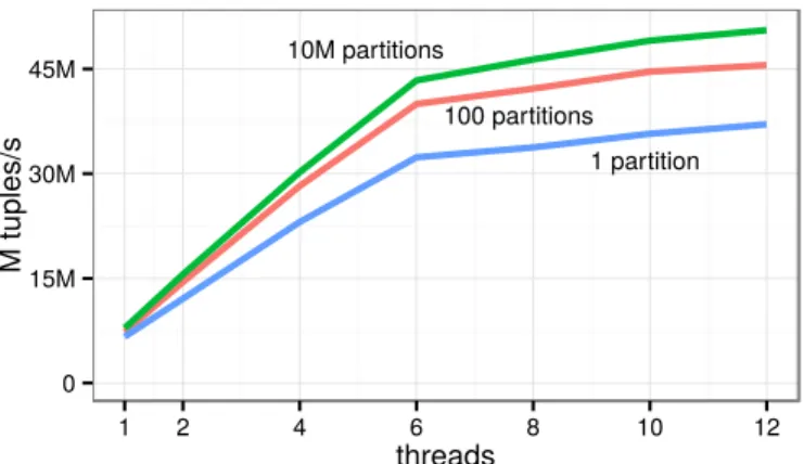
Figure 7: Single-threaded performance ofrankquery (with 100 partitions) 0 15M 30M 45M 1 2 4 6 8 10 12 threads M tuples/s 10M partitions 100 partitions 1 partition

Figure 8: Scalability ofrankquery

that, likerank, are also not affected by framing have similar per-formance; only aggregation functions with frames can be signifi-cantly more expensive (cf., Figure 12).

In the next experiment, we look at the scalability of our imple-mentation. We used different distributions for attributeacreating 10 million partitions, 100 partitions, or only 1 partition. The parti-tions have approximately the same size, so our algorithm chooses inter-partition parallelism with 10 million and 100 partitions, and intra-partition parallelism with 1 partition. Figure 8 shows that our implementation scales almost linearly up to 6 threads. After that, HyperThreading gives an additional performance boost.

5.4 Algorithm Phases

To better understand the behavior of the different phases of our algorithm, we measured the runtime with 12 threads and the speedups over single-threaded execution for the three phases of our algorithm. The results are shown in Table 2. The overall speedup

10M partitions 100 partitions 1 partition time speedup time speedup time speedup

phase [ms] [ms] [ms]

partition 46 2.5× 32 2.9× 32 2.3× sort 139 7.7× 184 6.7× 198 6.9× rank 12 7.0× 6 5.9× 10 7.4× = total 197 6.5× 223 6.2× 239 6.3× Table 2: Performance and scalability for the different phases of the window operator (rankquery)

(9)

0 15M 30M 45M

16 64 256 1024 4096 16384 65536

number of hash groups (log scale)

M tuples/s

10M partitions 100 partitions 1 partition

Figure 9: Varying the number of hash groups forrankquery.

is over 6×for all data distributions, which is a very good result with 6 cores and 12 HyperThreads. The majority of the query execution time is spent in the sorting and partitioning phases, be-cause the evaluation of therankfunction consists of a very fast and simple sequential scan. The table also shows that, all else be-ing equal, input distributions with more partitions result in higher overall performance. This is because sorting becomes significantly more expensive with larger partitions due to both asymptotic and caching reasons. The partitioning phase, on the other hand, be-comes only slightly more expensive with many partitions since we only partition into 1024 hash groups, which is always very efficient. When many threads are used for the partitioning phase, the avail-able memory bandwidth is exhausted, which explains the slightly lower speedup during partitioning. Of course, systems with higher memory bandwidth can achieve higher speedups. We also experi-mented with tuples larger than 16 bytes, which increases execution time due to higher data movement costs. However, the effect is not linear; using 64-byte tuples instead of 16-byte tuples reduces performance by 1.6×.

5.5 Skewed Partitioning Keys

In the previous experiments, each query used either inter-partition parallelism (100 or 10M partitions) or intra-partition parallelism (1 partition), but never a combination of the two. To show that inter-partition parallelism alone is not sufficient, we created an extremely skewed data set where 50% of all tuples belong to the largest par-tition, 25% to the second largest, and so on. Despite the fact that there are more partitions than threads, when we enforced inter-partition parallelism alone, we achieved a speedup of only 1.9× due to load imbalances. In contrast, when we enabled our auto-matic classification scheme that uses intra-partition parallelism for the largest partitions and inter-partition parallelism for the smaller partitions we measured a speedup of 5.9×.

5.6 Number of Hash Groups

So far, all experiments used 1024 hash groups. Figure 9 shows the overall performance of therankquery with a varying num-ber of hash groups. Having more hash groups can result in slower partitioning due to cache and TLB misses but faster sorting due to smaller partitions. Using 1024 hash groups results in performance close to optimal regardless of the number of partitions, because on modern x86 CPUs 1024 is small enough to allow for very cache-and TLB-friendly partitioning. Therefore, we argue that there is no need to rely on the query optimizer to choose the number of hash groups, and a value around 1024 generally seems to be a good setting. 0 15M 30M 45M 1 100 10K 1M

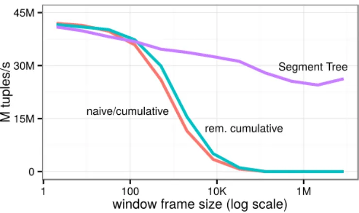
window frame size (log scale)

M tuples/s

rem. cumulative Segment Tree

naive/cumulative

Figure 10: Performance of sum query with constant frame bounds for different frame sizes

5.7 Aggregation with Framing

In the next experiment, we investigate the performance charac-teristics of the 4 different aggregation algorithms, which we im-plemented in C++ for this experiment because HyPer only imple-ments the cumulative and the Segment Tree algorithm. Using 12 threads, we execute the following query with different constants for the placeholder:

select sum(a) over

(order by b

rows between ? preceding and current row)

from r

By using different constants, we obtain queries with different frame sizes (from 1 tuple to 10M tuples). The frame “lags behind” the current row and should therefore be ideal for the removable cu-mulative aggregation algorithm, whereas the na¨ıve and cucu-mulative algorithms must recompute the result for each tuple.

Figure 10 shows that for very small frame sizes (<10 tuples), even the simple na¨ıve and cumulative algorithms perform very well. The Segment Tree approach is slightly slower in this range of frame sizes as it must pay the price of initially constructing the tree that is quite useless for such small frames. However, the over-head is quite small in comparison with the sorting and partitioning phases which dominate the execution time. For larger window sizes (10to10,000tuples), the na¨ıve and cumulative algorithms become very slow due to their quadratic behavior in this query. This also happens when we run such queries in PostgreSQL (not shown in the graph), which uses the cumulative algorithm.

As expected, the removable cumulative algorithm has good per-formance for the entire range, as the amount of work per tuple is constant and no ordered tree is necessary because the aggregation is a sum and not a minimum or maximum. However, for very large window sizes (>10,000 tuples), where the query, in effect, becomes a running sum over the entire partition, the removable cumulative algorithm does not scale and becomes as slow as single-threaded execution. The reason is that each thread must initially compute a running sum over the majority of all preceding tuples. We re-peated this experiment on a 60-core system, where the Segment Tree algorithm surpasses the removable cumulative algorithm for large frames with around 20 threads. The performance of Segment Tree traversal cost decreases only slightly with increasing frame sizes and is always high.

In the previous experiment, for each query the frame bound was a constant. In the experiment shown in Figure 11, the frame bound is an expression that depends on the current row and varies very

(10)

0 15M 30M 45M

1 100 10K 1M

window frame size (log scale)

M tuples/s

Segment Tree

rem. cumulative naive/cumulative

Figure 11: Performance of sum query with variable frame bounds for different frame sizes

0 50 100 150 200 2 4 8 16 32 64 128 256

fanout of Segment Tree (log scale) evaluation phase [ms] 1 preceding

unbounded preceding

Figure 12: Segment Tree performance forsumquery under varying fanout settings

strongly in comparison with the previous frame bound. Neverthe-less, the Segment Tree algorithm performs well even for large and extremely fluctuating frames. The performance of the other algo-rithms, in contrast, approaches 0 tuples/s for larger frame sizes due to quadratic behavior. We observed the same behavior with the commercial database system, whereas PostgreSQL does not sup-port such queries at all.

To summarize, the Segment Tree approach usually has higher overhead than the simpler algorithms, and it certainly makes sense to choose a different algorithmifthe query structure allows to stat-ically determine that this is beneficial. However, this not possible for many queries. The Segment Tree has the advantage of being very robust in all cases, and is dominated by the partitioning and sorting phases for all possible frame sizes. Additionally, the Seg-ment Tree always scales very well, whereas the other approaches cannot scale for large window sizes, which becomes more impor-tant on large systems with many cores.

5.8 Segment Tree Fanout

The previous experiments used a Segment Tree fanout of 16. The next experiment investigates the influence of the fanout of the Seg-ment Tree on the performance of aggregation and tree construction. Figure 12 uses the samesumquery as before but varies the fanout of the Segment Tree for two very extreme workloads. The time shown includes both the window function evaluation and Segment Tree construction. For queries where the frame size is very small (cf., curve labeled as “1 preceding”), using a higher fanout is

al-ways beneficial. The reason is that such queries build a Segment Tree but do not actually use it during aggregation due to the small frame size. For queries with large frames (cf., curve labeled as “un-bounded preceding”), a fanout of around 16 is optimal. For both query variants, the Segment Tree construction time alone (without evaluation, not shown in the graph) starts at 23ms with a fanout of 2 and decreases to 5ms with a fanout of 16 or higher.

Another advantage of a higher fanout is that the additional space consumption for the Segment Tree is reduced. For the example query, the input tuples use around 153MB. The additional space overhead for the Segment Tree with a fanout of 2 is 76MB (50%). The space consumption is reduced to 5MB (3.3%) with a fanout of 16, and to 0.6MB (0.4%) with a fanout of 128. Thus, a value close to 16 generally seems to be a good setting that offers a good balance between space consumption and performance.

6. RELATED WORK

Window functions were introduced as an (optional) amend-ment to SQL:1999 and were finally fully incorporated into SQL:2003 [25]. SQL:2011 added support for window functions for referring to neighboring tuples in a window frame. Oracle has been the first database system to implement window function sup-port in 1999, followed by IBM DB2 LUW in 2000. Successively, all major commercial and open source database systems, including Microsoft SQL Server (in 2005), PostgreSQL (in 2009), and SAP HANA followed5_.

As mentioned before, we feel there is a gap between the im-portance of window functions in practice and the amount of re-search on this topic in the database systems community, for exam-ple in comparison with other analytic SQL constructs like rollup and cube [13]. An early Oracle technical report [8] contains mo-tivating query examples, optimization opportunities, and parallel execution strategies for window functions. In a more recent pa-per, Bellamkonda et al. [9] observed that using partitioning only to achieve good scalability is not sufficient if the number of dis-tinct groups is lower than the desired degree of parallelism. They proposed to artificially enlarge the partitioning key with additional attributes (“extended distribution keys”) to achieve a larger number of partitions and therefore increased parallelism. However, this ap-proach incurs additional work due to having an additional window consolidator phase and relies on cardinality estimates. We sidestep these problems by directly and fully parallelizing each phase of the window operator and by using intra-partition parallelism when necessary.

There are a number of query optimization papers that relate to the window operator. Cao et al. [12] focus on optimizing multiple window functions occurring in one query. They found that often the majority of the execution time for the window operator is spent in the partitioning and sorting phases. Therefore, it is often possible to avoid some of the partitioning and/or sorting work by optimizing the order of the window expressions. The paper shows that find-ing the optimal sequence is NP-hard and presents a useful heuristic algorithm for this problem. Though the window operator is very useful its own right, other papers [26, 7] propose to introduce win-dow expressions for de-correlating subqueries. In such scenarios, a fast implementation of the window operator is important even for queries that do not originally contain window functions. Due to a different approach for unnesting [20], HyPer currently does not introduce window operators when unnesting queries. In the fu-ture, we plan to investigate whether might be beneficial with our 5_{Two widely-used systems that do not yet offer window function} support are MySQL/MariaDB and SQLite.

(11)

approach. Window functions have also been used to speed up the translation of XQuery to SQL [10].

Yang and Widom [24] introduced the Segment B-Tree for tem-poral aggregation, which is very similar to our Segment Tree except that we do not need to handle updates and can therefore represent the structure more efficiently without pointers.

7. SUMMARY AND FUTURE WORK

We have presented an algorithm for window function computa-tion that is very efficient in practice and avoids quadratic runtime in all cases. Furthermore, we have shown how to execute window functions in parallel on multi-core CPUs, even when the query has no partitioning clause. We have demonstrated both the high perfor-mance and the excellent scalability in a number of experiments that cover very different query types and input distributions.

Since the literature on window functions is very sparse, there are many possible directions for future work. In this paper, we focused on execution in main-memory database systems, although our core algorithmic ideas also apply to disk-based implementa-tions. It would be interesting to investigate which changes would be required in that setting. Another possible optimization would be to focus on Non-Uniform Memory Access (NUMA) systems.

Acknowledgments

We would like to thank the reviewers for their constructive com-ments to improve this work.

8. REFERENCES

[1] http://docs.oracle.com/database/121/ DWHSG/analysis.htm. [2] http://msdn.microsoft.com/en-us/library/ ms189461(v=sql.120).aspx. [3] http://www-01.ibm.com/support/ knowledgecenter/SSEPGG_10.5.0/com.ibm. db2.luw.sql.ref.doc/doc/r0023461.html. [4] http://help.sap.de/hana/SAP_HANA_SQL_ and_System_Views_Reference_en.pdf. [5] http://www.postgresql.org/docs/9.4/ static/tutorial-window.html. [6] https://www.monetdb.org/Documentation/ Manuals/SQLreference/WindowFunctions. [7] S. Bellamkonda, R. Ahmed, A. Witkowski, A. Amor,

M. Za¨ıt, and C. C. Lin. Enhanced subquery optimizations in Oracle.PVLDB, 2(2):1366–1377, 2009.

[8] S. Bellamkonda, T. Bozkaya, B. Ghosh, A. Gupta, J. Haydu, S. Subramanian, and A. Witkowski. Analytic functions in Oracle 8i. Technical report, Oracle, 2000.

[9] S. Bellamkonda, H.-G. Li, U. Jagtap, Y. Zhu, V. Liang, and T. Cruanes. Adaptive and big data scale parallel execution in Oracle.PVLDB, 6(11):1102–1113, 2013.

[10] P. Boncz, T. Grust, M. van Keulen, S. Manegold, J. Rittinger, and J. Teubner. Pathfinder: XQuery - the relational way. In VLDB, pages 1322–1325, 2005.

[11] P. Boncz, M. Zukowski, and N. Nes. MonetDB/X100: Hyper-pipelining query execution. InCIDR, pages 225–237, 2005.

[12] Y. Cao, C.-Y. Chan, J. Li, and K.-L. Tan. Optimization of analytic window functions.PVLDB, 5(11):1244–1255, 2012. [13] V. Harinarayan, A. Rajaraman, and J. D. Ullman.

Implementing data cubes efficiently. InSIGMOD, pages 205–216, 1996.

[14] D. Inkster, M. Zukowski, and P. Boncz. Integration of VectorWise with Ingres.SIGMOD Record, 40(3):45–53, 2011.

[15] A. Kemper and T. Neumann. HyPer: A hybrid OLTP&OLAP main memory database system based on virtual memory snapshots. InICDE, pages 195–206, 2011.

[16] M. Kornacker, A. Behm, V. B. T. Bobrovytsky, C. Ching, A. Choi, J. Erickson, M. Grund, D. Hecht, M. Jacobs, I. Joshi, L. Kuff, D. Kumar, A. Leblang, N. Li, I. Pandis, H. Robinson, D. Rorke, S. Rus, J. Russell, D. Tsirogiannis, S. Wanderman-Milne, and M. Yoder. Impala: A modern, open-source SQL engine for Hadoop. InCIDR, 2015. [17] V. Leis, P. Boncz, A. Kemper, and T. Neumann.

Morsel-driven parallelism: A NUMA-aware query evaluation framework for the many-core age. InSIGMOD, pages 743–754, 2014.

[18] R. O. Nambiar and M. Poess. The making of TPC-DS. In VLDB, pages 1049–1058, 2006.

[19] T. Neumann. Efficiently compiling efficient query plans for modern hardware.PVLDB, 4:539–550, 2011.

[20] T. Neumann and A. Kemper. Unnesting arbitrary queries. In BTW, pages 383–402, 2015.

[21] T. Neumann and V. Leis. Compiling database queries into machine code.IEEE Data Eng. Bull., 37(1):3–11, 2014. [22] F. Putze, P. Sanders, and J. Singler. MCSTL: the multi-core

standard template library. InPPOPP, pages 144–145, 2007. [23] O. Shalev and N. Shavit. Split-ordered lists: Lock-free

extensible hash tables.J. ACM, 53(3):379–405, 2006. [24] J. Yang and J. Widom. Incremental computation and

maintenance of temporal aggregates. InICDE, pages 51–60, 2001.

[25] F. Zemke. What’s new in SQL:2011.SIGMOD Record, 41(1):67–73, 2012.

[26] C. Zuzarte, H. Pirahesh, W. Ma, Q. Cheng, L. Liu, and K. Wong. WinMagic: Subquery elimination using window aggregation. InSIGMOD, pages 652–656, 2003.

APPENDIX

A. Example Window Function Queries

To motivate the usefulness and versatility of the window operator we show a number of queries that can be stated elegantly and effi-ciently using window functions.

Determine medalists for an Olympic competition (the same num-ber of points results in the same medal, the there are two gold medals no silver medal is not awarded):

select name, (case rank when 1 then ’Gold’ when 2 then ’Silver’

else ’Bronze’ end)

from (select name, rank() over w as rank

from results

window w as (order by points desc))

where rank <= 3

For each customer purchase determine the sum of all orders of the customer in the same calendar month:

select customer, time, sum(amount) over

(partition by customer

order by

rows between time - extract(days from time)

and current row)

(12)

The rate of change for each measurement in comparison with the previous measurement (e.g., “transactions per second”) :

select time,

(value - lag(value) over w) / (time - lag(time) over w)

window w as (order by time)

B. Window Functions with Framing

The following code shows the algorithmic template for window functions that are affected by framing:

1 evalOverFrame(begin, end)

2 pBegin = findPartitionBegin(0, begin+1) 3 pEnd = findPartitionEnd(begin)

4 for (pos from begin below end) 5 if (pos = pEnd)

6 pBegin = pos

7 pEnd = findPartitionEnd(pos) 8 wBegin = findWindowBegin(pos,pBegin) 9 wEnd = findWindowEnd(pos, pEnd) 10 result[pos] = eval(wBegin, wEnd)

The code computes the result for a sub-range in a hash group (from

beginbelowend). This interface allows to parallelize window function evaluation within a hash group by assigning threads to different ranges, e.g., using aparallel forconstruct that dy-namically distributes the range of values between threads. Since a hash group can contain multiple partitions, the code starts by com-puting the partition bounds (line 2 and 3), and then updates them as needed (lines 5, 6, and 7).

C. Segment Tree Traversal

The following pseudo code computes the aggregate for the range frombeginbelowendusing a Segment Tree:

1 traverseSTree(levels, begin, end) 2 agg = initAggregate()

3 for (level in levels)

4 parentBegin = begin / fanout 5 parentEnd = end / fanout 6 if (parentBegin = parentEnd) 7 for (pos from begin below end)

8 agg = aggregate(level[pos])

9 return agg

10 groupBegin = parentBegin * fanout 11 if (begin != groupBegin)

12 limit = groupBegin + fanout 13 for (pos from begin below limit)

15 parentBegin = parentBegin + 1 16 groupEnd = parentEnd * fanout 17 if (end != groupEnd)

18 for (pos from groupEnd below end)

20 begin = parentBegin 21 end = parentEnd

Line 3 loops over the levels of the Segment Tree starting at the bottom-most level and proceeding upwards. In line 4 and 5 the par-ent par-entries ofbeginandendare computed using integer division, which can be implemented as bit shifting if fanout is a power of 2. If the parent entries are equal, the range of values betweenbegin

andendis aggregated and the search terminates (lines 6-9). Oth-erwise, the search continues at the next level with the parent nodes becoming the newbeginandendboundaries. It is first neces-sary, however, to aggregates any “protruding” values at the current level (lines 10-18).

D. Window Functions without Framing

In Section 4.4 we show the pseudo code for therank function. Here, we provide two additional examples for window functions that are always evaluated on the entire partition:

//relative rank

percent_rank(begin, end)

pBegin = findPartitionBegin(0, begin+1) pEnd = findPartitionEnd(begin)

firstPeer = findFirstPeer(pBegin, begin) rank = (firstPeer-pBegin)+1

pSize = pEnd - pBegin

result[begin] = (rank-1) / (pSize-1)

for (pos from begin+1 below end)

if (pos = pEnd) pBegin = pos pEnd = findPartitionEnd(pos) pSize = pEnd-pBegin if (isPeer(pos, pos-1)) result[pos] = result[pos-1] else rank = pos+1

result[pos] = (rank-1) / (pSize-1)

// evaluate expr at preceding row lag(expr, offset, default, begin, end)

pBegin = findPartitionBegin(0, begin+1) pEnd = findPartitionEnd(begin)

for (pos from begin below end)

if (pos = pEnd) pBegin = pos pEnd = findPartitionEnd(pos) if (pos-offset < pBegin) result[pos] = default else result[pos] = expr(pos-offset)

E. Distinct Aggregates

Distinct aggregates, which in contrast to normal aggregates cannot be used with framing, are best executed without using the window operator. Instead, distinct aggregates can be executed efficiently using normal aggregation and an additional join. For example, the query

select sum(distinct x) over (partition by y)

from r

is equivalent to:

select d.cd from r,

(select sum(distinct x) as cd, y

from r group by y) d

where r.y = d.y

The same transformation, which avoids the sorting phase, is also beneficial for non-distinct aggregates where the frame always en-compasses the entire partition.