A Pure Cumulant-Based Method with Low Computational
Complexity for Classification and Localization of Multiple Near
and Far Field Sources Using a Symmetric Array
Amir Masoud Molaei1, *, Ali Ramezani Varkani2, and Mohammad Reza Soheilifar2
Abstract—The authors propose a new method based on spatial cumulants for estimating the parameters of multiple near-field and far-field sources. The Toeplitz property used in some studies is not applicable to fourth-order statistics to separate sources components. Therefore, in this paper, a method is proposed to compute output cumulants of specified sensors in special arrangements, by which the components of the near-field and the far-field sources are effectively separated using differencing. The angle and range estimations, as well as the classification of the sources, are obtained based on the data from two spatial cumulant matrices. One of them contains the angle information of all sources, and the other only contains the information of near-field sources. The parameters extraction algorithm is based on the ESPRIT technique; therefore, the proposed method does not require any spectral search. This leads to a significant reduction in computational complexity. Unlike some approaches, the proposed method does not suffer from array aperture loss. Also, the parameters pairing procedure is done automatically. Analysis and simulation results confirm the good performance of the proposed method in terms of computational complexity, estimation accuracy, correct classification of signals, and aperture loss.
1. INTRODUCTION
The direction-of-arrival (DOA) estimation is one of the practical and progressive applications in the field of array signal processing. The main purpose of the DOA estimation is to find the direction of the signals impinging on an antenna array [1]. These signals can be electromagnetic or acoustic waves. The necessity of locating and tracking signal sources in military and civilian applications (such as search and rescue, sonar, seismology, and wireless emergency call locating) shows the importance of DOA estimation. An array can be designed to detect incoming signals so that it only accepts signals from certain directions and rejects ones that are declared as interference.
In many array processing applications, the wave-front is assumed to be planar; in other words, the sources are located in the far-field (FF) of the array. In this case, the task of locating the source is limited to estimating DOAs only. Although plane wave assumption can simplify modeling and processing, such a hypothesis is not valid in practical applications of near-field (NF), as a result, will lead to error in the analysis. When the source is located in the NF or in the Fresnel region of the array aperture, the shape of the spherical wave-front varies nonlinearly with the array position and is characterized by the angle and the range parameters [2]. As a result, the conventional DOA estimation algorithms for far-field sources (FFSs) are not applicable to localization of near-field sources (NFSs). In addition, in some practical applications such as seismic exploration [3], electronic supervision [4], speaker localization
Received 10 May 2019, Accepted 8 July 2019, Scheduled 9 October 2019
* Corresponding author: Amir Masoud Molaei ([email protected]).
using a microphone array, and guidance system [5, 6], any source can be located in FF or NF. Under such circumstances, conventional methods are encountered with serious drawbacks, since these methods inherently require pure FF or NF signals. Accordingly, in recent years, there has been growing interest in the issue of mixed sources localization.
An efficient method for localization of mixed FFSs and NFSs was first proposed by a two-stage MUSIC algorithm [7], using fourth-order cumulants (FOCs) and spectral search. An algorithm called oblique projection MUSIC was proposed in [8] using second-order statistics (SOS). In [9], an ESPRIT-MUSIC-like method has been developed based on the third-order cyclic moment. Despite the relatively less computational complexity, the reduced range estimation accuracy and some limiting hypotheses are considered as disadvantages in the work [9]. The authors of the study [10] extended the array aperture by using a sparse linear array. Compared to previous algorithms, research [10] has a moderate computational complexity and higher resolution and also has improved the estimation accuracy of parameters. However, it suffers from the problem of spurious peaks concerning range estimation. A method based on constructing spatial-temporal cumulants is presented in [11], which does not need to know the number of sources. Based on the generalized ESPRIT (GESPRIT) algorithm [12], several methods have been proposed to localize mixed sources [6, 13–15]. Compared to other SOS-based methods, the algorithm [13] has improved the estimation accuracy and also made a more reasonable classification of signals types. The covariance differencing method presented in [14, 15] provides a reasonable classification. For GESPRIT-based algorithms, the maximum number of resolvable NFSs is less than half of the array’s sensors [16]. In [17], an SOS-based method is proposed to estimate the DOA, range, and frequency parameters, which avoids multi-dimensional spectral search. The use of the mixed second and fourth order statistics with applying the MUSIC technique is considered in research [18], which provides a reasonable classification. However, it sets strict limits on the DOA intervals of incoming signals. In the study [19], a mixed order statistics method based on cumulant matrix reconstruction and the use of MUSIC spectrum has been presented, which provides good accuracy.
All of the above methods require heavy computations of spectral search. In addition, the methods [7, 11, 18, 19] have a higher computational burden due to the construction of fourth-order statistics (FOS) matrices along with spectral search. On the other hand, the aperture loss that appears in works [6, 8, 9, 14, 15, 19] is another issue that should be considered about the number of sensors. Also, in the case of NFSs, in addition to the DOA and range estimations, the pairing between these two parameters should also be made. The differencing operation presented in [14, 15] is valid only for SOS, and according to what we will show in the text, for FOS-based methods, the Toeplitz property will no longer help to separate the FF and NF components.
What will be presented in this paper is an algorithm that, in addition to efficient separation of the FF and NF components in the cumulant domain, estimates the parameters of the mixed NFSs and FFSs without the need for a pairing process and with the lowest aperture loss. The use of high-order statistics, in addition to increasing the estimation accuracy, also allows saving the number of sensors [20]. In addition, FOCs are not sensitive to any kind of Gaussian noise. In the proposed method, the signals are received by a symmetric uniform linear array (ULA). Five special cumulants are defined, and five corresponding matrices are constructed based on the received data. The first matrix only contains the angle information, and the sources’ DOAs are extracted from it. Four other matrices, pairwise, contain common FF information. By two differencing operations, FFSs information is eliminated. The information needed to classify sources and estimate the NFSs parameters is obtained by providing an ESPRIT-based method.
The rest of this paper is organized as follows. In Section 2, the mathematical model of the data and main assumptions are expressed. In Section 3, the proposed algorithm is completely explained. Section 4 deals with the performance analysis of the proposed algorithm. Simulations and their results are presented in Section 5. Conclusions are given in Section 6. Also, details of some equations and proofs are given in the Appendix.
Notation: Throughout the paper, superscripts T, H, and ∗ represent the transpose, conjugate transpose, and complex conjugate, respectively. Symbols ˆx, E{x}, and x stand for the estimation, mathematical expectation, and floor of x, respectively. Jx×y represents the matrix of ones of sizex×y.
2. DATA MODEL
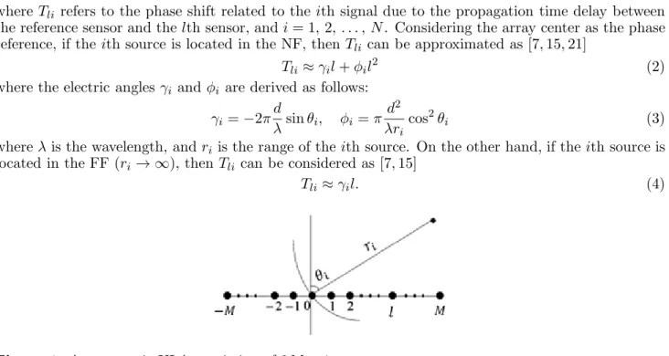
ConsiderNuncorrelated narrowband sources includingNN NFSs andNF FFSs. The signals transmitted by these sources impinge on a symmetric ULA consisting of 2M + 1 sensors with element spacing
d from the directions θ1, θ2, . . . , θN (Fig. 1). Each element is denoted by an index l, where l =
−M, . . . ,0, . . . , M. The array steering vector for the ith incoming signal and the lth sensor is defined by
ali =ejTli (1) where Tli refers to the phase shift related to the ith signal due to the propagation time delay between the reference sensor and thelth sensor, andi= 1,2, . . . , N. Considering the array center as the phase reference, if theith source is located in the NF, then Tli can be approximated as [7, 15, 21]
Tli≈γil+φil2 (2) where the electric angles γi and φi are derived as follows:
γi =−2πdλsinθi, φi=π d 2
λri cos 2
θi (3)
whereλis the wavelength, andri is the range of theith source. On the other hand, if theith source is located in the FF (ri→ ∞), thenTli can be considered as [7, 15]
Tli≈γil. (4)
Figure 1. A symmetric ULA consisting of 2M+ 1 sensors.
With a proper sampling rate, thekth sample of the signal observed by the lth sensor is expressed as [22]
xl(k) = N
i=1
si(k)ejTli+nl(k), k= 1, . . . , Ns (5)
where Ns, si(t), and nl(t) are the number of snapshots, signal of the ith source, and noise of the lth sensor, respectively. Without the loss of generality, we assume that the first NN signals are received from the NF and the remaining signals from the FF, so Eq. (5) can be rewritten as
xl(k) = NN
i=1
si(k)ej(γil+φil2) + N
i=NN+1
si(k)ejγil+n
l(k). (6)
In matrix form, the array output vector is expressed as
x(k) =A s(k) +n(k) (7)
whose vectors and matrices are determined by
x(t) = [x−M(t) . . . x0(t) . . . xM(t)]T
s(t) =sTN(t) sTF (t)T
sN(t) = [s1(t) s2(t) . . . sNN(t)]T
sF (t) = [sNN+1(t) sNN+2(t) . . . sN(t)]T
n(t) = [n−M(t) . . . n0(t) . . . nM(t)]T
where sN(t) ∈CNN×1, s
F(t) ∈CNF×1 and n(t) ∈C(2M+1)×1 are the source vector of the NF and FF signals, and the additive Gaussian noise vector with mean zero. A∈C(2M+1)×N is the steering matrix and can be written as
A= [AN AF], AN = [a1 a2 . . . aNN]
AF = [aNN+1 . . . aN], ai= [a−Mi a−M+1i . . . aMi]T
(9)
whereali can be determined by Eqs. (1), (2), and (4). The following basic hypotheses are assumed to hold: 1- The array is calibrated, and the matrix A is full rank.
2- The signals{si(t)}Ni=1are statistically mutually independent, narrowband stationary processes with nonzero kurtosis.
3- Sensor noise is the additive (white or color) Gaussian one and statistically independent of sources signals.
4- The sensor array is a ULA arranged by element spacing d ≤ λ/4, in order to avoid the phase ambiguity [23].
5- The number of elements satisfies both 2M + 1> N and 2M+ 1≥NN + 2. 6- Signals’ DOAs are different.
3. PROPOSED METHOD
In this section, first, some special cumulant matrices are defined. The proposed method is then fully explained.
3.1. Definition and Construction of Special Cumulant Matrices
Since the proposed method uses FOS, we consider five cross-cumulant functionsc4x,1(¯u,v¯),c4x,2(u, v),
c4x,3(u, v),c4x,4(u, v) andc4x,5(u, v) for the array output stationary signals with a common zero time lag and different sensor lags in the following form:
c4x,1(¯u,v¯) =Cum
x∗u¯(k), xv¯(k), x∗−v¯(k), x−u¯(k)
c4x,2(u, v) =Cum
x∗u(k), xu+1(k), x∗v+1(k), xv(k)
c4x,3(u, v) =Cum{x∗u(k), xu+1(k), x∗v(k), xv−1(k)}
c4x,4(u, v) =Cum
x∗u−1(k), xu(k), x∗−v(k), x1−v(k)
c4x,5(u, v) =Cum
x∗u(k), xu+1(k), x∗−v(k), x1−v(k)
(10)
where ¯u,v¯∈ [−M, M] and u, v ∈ [−M+ 1, M−1]. According to assumptions 2 and 3, the result of the cumulants of Eq. (10) can be written as (see Appendix A for more details)
c4x,1(¯u, ¯v) = N
i=1
csie−j2¯uγiej2¯vγi
c4x,2(u, v) = NN
i=1
csiej2uφie−j2vφi+
N
i=NN+1
csi
c4x,3(u, v) = NN
i=1
csiej2(u+1)φie−j2vφi+
N
i=NN+1
csi
c4x,4(u, v) = NN
i=1
csiej2uφie−j2vφiej2γi+
N
i=NN+1
csiej2γi
c4x,5(u, v) = NN
i=1
csiej2(u+1)φie−j2vφiej2γi+
N
i=NN+1
csiej2γi
wherecsi =Cum{s∗i(t), si(t), s∗i(t), si(t)}is the kurtosis related to theith signal. According to Eq. (11)
and by collecting all sensor lags, we can construct the complex cross-cumulant matrices of the sensors in the following form:
C1 =BCsBH, C2 =DCsDH, C3=DΦCsDH
C4 =DΥCsDH, C5=DΦΥCsDH.
(12)
Equation (13) gives the value of the u,vth element of matrix C1 according to the definitions
u = ¯u+M + 1 and v = ¯v +M + 1. Also, by defining ˜u = u+M and ˜v = v+M, the (˜u,v˜)th element of matrices C2, C3, C4, and C5 can be obtained from Eq. (13) (see Appendix A for their practical estimation)
C1
u,v=Cum x∗u(t), xv (t), x∗
N−v+1(t), xN−u+1(t)
C2(˜u, ˜v) =Cum
x∗u˜+1(t), xu˜+2(t), x∗˜v+2(t), xv˜+1(t)
C3(˜u, ˜v) =Cum
x∗u˜+1(t), xu˜+2(t), x∗˜v+1(t), xv˜(t)
C4(˜u, ˜v) =Cum
x∗u˜(t), xu˜+1(t), xM∗ −˜v(t), xM+1−˜v(t)
C5(˜u, ˜v) =Cum
x∗u˜+1(t), xu˜+2(t), x∗M−v˜(t), xM+1−˜v(t)
(13)
where u,v ∈ [1,2M+ 1] and ˜u,v˜ ∈ [1,2M −1]. Therefore, the first matrix of Eq. (12) is of size (2M + 1)×(2M+ 1), and the last four matrices are of size (2M −1) ×(2M−1). Cs ∈ RN×N,
Υ∈CN×N and Φ∈CN×N are the diagonal matrices defined in the following form:
Φ= diag
ej2φ1, ej2φ2, . . . , ej2φNN,1, . . . , 1
Υ= diagej2γ1, ej2γ2, . . . , ej2γN
Cs= diag [cs1, cs2, . . . , csN].
(14)
In this way, B∈C(2M−1)×N is obtained by
B=
⎡ ⎢ ⎢ ⎢ ⎣
ej2(2M)γ1 ej2(2M)γ2 . . . ej2(2M)γN
ej2(2M−1)γ1 ej2(2M−1)γ2 . . . ej2(2M−1)γN
..
. ... . .. ...
1 1 . . . 1
⎤ ⎥ ⎥ ⎥
⎦. (15)
Also, matrix D ∈ C(2M−1)×N is of rank NN + 1 (according to assumption 6), in which the elements of the last NF columns are equal to 1, and the elements of the first NN columns contain information about φi. D is obtained by
D=DN J(2M−1)×NF
DN =
⎡ ⎢ ⎢ ⎢ ⎣
1 . . . 1
ej2φ1 . . . ej2φNN
..
. . .. ...
ej2(2M−2)φ1 . . . ej2(2M−2)φNN
⎤ ⎥ ⎥ ⎥ ⎦.
(16)
3.2. Sources’ DOA Estimation
In the proposed method, the information of the last four matrices of Eq. (12) alone is not sufficient to find the DOA of the FFSs and to classify the signals types. The first matrix only contains the DOA information, which we only use in this section.
We form two overlapping matrices C11∈C2M×(2M+1) andC12∈C2M×(2M+1) as
where C11 and C12 consist of the first 2M and the last 2M rows of the Hermitian matrix C1, respectively. B1 ∈ C2M×N and B2 ∈ C2M×N, respectively, include the first 2M and the last 2M rows of B, and they hold the following equation:
B2=B1ψ (18)
where ψ = diag[e−j2γ1, . . . , e−j2γN] contains the angle information of all sources. According to
assumptions 5 and 6, B1 and BH are full column and full row rank, respectively. We form the angle
estimation matrix as
CA=CH11C11
−1
CH11C12=
BHB−1BHψB. (19)
By applying the eigenvalue decomposition (EVD) to CA, we have
CA=UΣU−1 (20)
where Σ = diag[σ1, . . . , σ2M+1] is a diagonal matrix with the eigenvalues arranged as |σ1| ≥ . . . ≥
|σN| > |σN+1| > . . . > |σ2M+1|. A part of U ∈ C(2M+1)×(2M+1) contains N eigenvectors related to eigenvalues σ1, . . . , σN, which spans the signal subspace ofCA.
The sources’ DOAs can easily extract from Eq. (21)
ˆ
θi = arcsin
λ∠σ
i 4πd
, i= 1, . . . , N (21)
where σi = e−j2ˆγi. We define the angles estimation vector as θˆ= [ˆθ1, . . . , θˆN]. Equation (21) alone
cannot determine which DOAs belong to NFSs and which belong to the FFSs.
3.3. NF and FF Components Separation by Differencing in the Cumulant Domain
In this section, a new method is proposed for separating the components of the NF and the FF in the cumulant domain. With respect to Eq. (13), each of the last four matrices in Eq. (12) can be written as the sum of two cumulant matrices, one containing only the information of the NF components, and the other one only contains FF information, namely
C2=CN1+CF1, C3 =CN2+CF1
C4=CN3+CF2, C5 =CN4+CF2.
(22)
According to Appendix B, both NF and FF parts of the above matrices are Toeplitz. Therefore, the use of algorithms such as [14, 15], which take advantage of being Toeplitz of the FF covariance matrix and being non-Toeplitz of the NF covariance matrix for the separation of components, cannot be implemented here for FOS.
Now, by simple differencing between the pair of matricesC2,C3 and C4,C5, we have
C32=C3−C2 =CN2−CN1
C54=C5−C4 =CN4−CN3.
(23)
The matrices C32 ∈ C(2M−1)×(2M−1) and C54 ∈ C(2M−1)×(2M−1) only contain the information of the NF components and are given in Eq. (24).
C32=j2 ·
⎡ ⎢ ⎢ ⎢ ⎢ ⎢ ⎢ ⎢ ⎢ ⎢ ⎢ ⎢ ⎢ ⎣
cs1ejφ1sinφ1+. . . +csNNejφNN sinφNN
. . . cs1e
−j(4M−5)φ1sinφ 1+. . . +csNNe−j(4M−5)φNNejφNN sinφNN
cs1ej3φ1sinφ1+. . . +csNNej3φNN sinφNN
. . . cs1e
−j(4M−7)φ1sinφ 1+. . . +csKNe−j(4M−7)φNN sinφNN
..
. . .. ...
cs1ej(4M−3)φ1sinφ1+. . . +csNNej(4M−3)φNN sinφNN
. . . cs1e
jφ1sinφ 1+. . . +csNNejφNN sinφNN
C54=j2·
⎡ ⎢ ⎢ ⎢ ⎢ ⎢ ⎢ ⎢ ⎢ ⎢ ⎢ ⎢ ⎣
cs1ejφ1ej2γ1sinφ1+. . . +csKNejφNNej2γNN sinφNN
. . . cs1e
−j(4M−5)φ1ej2γ1sinφ 1+. . . +csNNe−j(4M−5)φNNejγNN sinφNN
cs1ej3φ1ej2γ1sinφ1+. . . +csNNej3φNNej2γNN sinφNN
. . . cs1e
−j(4M−7)φ1ej2γ1sinφ 1+. . . +csKNe−j(4M−7)φNNejγNN sinφNN
..
. . .. ...
cs1ej2(2M−1)φ1ej2γ1sinφ1+. . . +csKNej2(2M−1)φNNej2γNN sin
φNN . . .
cs1ej2φ1ej2γ1sinφ1+. . . +csNNej2φNNejγNN sinφNN
⎤ ⎥ ⎥ ⎥ ⎥ ⎥ ⎥ ⎥ ⎥ ⎥ ⎥ ⎥ ⎦
(24)
In this way, we are able to separate the pure NF components from the entire data in the cumulant domain. In the next section, we will use this information to estimate the range and DOA of NFSs.
3.4. NFSs DOA Identification and Range Estimation
In the previous section, we showed how we can obtain pure NF information from the observed data using the cumulant differencing. The difference matricesC32andC54can be decomposed as the multiplication of matrices DN,CsN,ΦN, and ΥN as
C32=DNΦNCsNDHN, C54=DNΦNΥNCsNDHN (25) whereCsN,ΦN,ΥN ∈CNN×NN are derived from Eq. (26)
CsN = diag
cs1, cs2, . . . , csNN
ΦN =j2·diag
ejφ1sinφ1, ejφ2sinφ2, . . . , ejφNN sinφNN
ΥN = diagej2γ1, ej2γ2, . . . , ej2γNN.
(26)
Given assumptions 1 and 6, in order forDN to be a full column rank matrix, it is necessary and sufficient that the number of sensors satisfies 2M+ 1≥NN + 2; this condition corresponds to assumption 5.
The two equations expressed in Eq. (25) can be considered as the basic equations of ESPRIT [24]. Therefore, we define the NF parameters estimation matrix CN ∈C(2M−1)×(2M−1) as
CN =C32
CH54C54
−1
CH54. (27)
According to assumption 5,DN is full column rank, and it can easily be shown thatDHN ∈CNN×(2M−1) is a full row rank matrix [25]. On the other hand, according to assumption 2,CsN has no zero singular value, and there are no two identical elements on the main diagonal ofΦN andΥN (except forθ=±90◦). Therefore, we can rewrite Eq. (27) as
CN =DNΥ−N1DHNDN−1DHN (28)
whereBHN† is full column rank.
Given thatDN is full column rank, to estimate the electric angles of the NFSs, we need to apply EVD toCN
CN =QΛQ−1= [q1, . . . , q2M−1] diag [μ1, . . . , μ2M−1] [q1, . . . , q2M−1]−1 (29) whereΛ∈C(2M−1)×(2M−1) is a diagonal matrix with eigenvalues arranged as μ1 ≥. . .≥μN > μN+1 =
. . . = μ2M−1 = 0, and Q ∈ C(2M−1)×(2M−1) is the matrix of eigenvectors with column vectors qi (i = 1, . . . , 2M−1). NN non-zero eigenvalues (from N non-zero eigenvalues) obtained from the EVD of CN give an estimate of the diagonal elements of the matrix Υ−N1 (that is e−j2ˆγi, i = 1, . . . , NN)
containing the information of the NFSs’ DOA. Therefore, we can choose the NFSs’ DOAs from the values estimated by Eq. (30)
ˆ
ϑi= arcsin
λ∠μi
4πd
NN common values between the ˆϑis in Eq. (30) and the angles estimated in θˆare considered as valid DOAs of the NFSs, which form the vector θˆN ∈ R1×KN. The rest of the elements of vector θˆare considered as DOAs of the FFSs.
On the other hand, the NN eigenvectors qi (i = 1, . . . , NN), corresponding to the valid ˆϑis, can give an estimate of DN. By dividing the elements of the m+ 1th row of qi by the corresponding elements of the mth row (m= 1, . . . , 2M−3), we can extract an estimate ofφi as
ˆ
φi = 1
2 1 2M−3
2M−3
m=1
qm+1, i
qm, i , i
= 1, . . . , N
N (31)
where qm, i is the element of the mth row of qi. Given Eqs. (3) and (31), we can calculate the NFSs’ range by
ˆ
ri =
πd2cosθˆi
λφˆi , i
= 1, . . . , N
N (32)
where ˆθi is themth member ofθˆN.
4. ANALYSIS AND DISCUSSION
In this section, we analyze and discuss the proposed algorithm from four ways including computational complexity, aperture loss, parameters pairing, and NFS localization at the same angle with the FFS.
4.1. Computational Complexity
Here, we compare computational complexity [26] of the proposed method, considering the major multiplications.
The method [7] requires constructing two fourth-order matrices with dimensions (2M + 1) × (2M + 1) and (4M+ 1)×(4M+ 1), applying EVD to them, and performing the one-dimensional MUSIC spectral search for direction estimation. In addition, the range estimation requires N times the EVD implementation on matrices of size (8M+ 5)×(8M + 5). Therefore, the number of operations required in the work [7] is equal to
9 (2M + 1)2Ns+ 9 (4M+ 1)2Ns+43(2M + 1)3+43(4M+ 1)3+34N(8M+ 5)3+180Δ
θ (2M+ 1) 2 (33)
where Δθ is the angle search step in degree.
The method [8] involves the construction of one covariance matrix of size (2M+ 1)×(2M + 1) and another covariance matrix of size (M+ 2)×(M+ 2) (by selecting M2+1as the number of overlapping subvectors), applying EVD to them, spectral search implementation for the DOA estimation, and N
times the spectral search implementation for range. Therefore, the number of operations required in [8] is equal to
(2M+ 1)2Ns+ (M+ 2)2Ns+ 4
3(2M+ 1) 3
+1
3(M+ 2) 3
+180
Δθ (2M + 1) 2+
N
2D2λ−0.62
D3λ
Δr (2M + 1)
2 (34)
where Δr is the range search step in terms of wavelength.
The method [15] constructs one (2M + 1)×(2M+ 1) covariance matrix, computes its SVD, along with the SVD of the covariance difference matrix (with dimension (2M + 1)×(2M+ 1)) and the FF matrix (with dimension (2M+ 1)×(2M + 1)). In addition, two spectral searches for the angle andNN times spectral search for the range are required. Therefore, the sum of multiplications in [15] is equal to
(2M+ 1)2Ns+ 4 (2M+ 1)3+720Δ θM
2+180
Δθ (2M + 1) 2
+NN
2D2λ−0.62
D3λ
Δr (2M+ 1)
2
The method [11] constructsLcumulant matrices and one covariance matrix with dimensions (2M + 1)× (2M + 1). Also, it constructs two other matrices, one with dimension (2M+ 1)×(2M + 1) (requiring the product ofL cumulant matrices with their Hermitian) and the other one with dimension (2M + 1)×L
(requiring the product of L cumulant matrices with the virtual steering vector). It also requires an EVD (on aL×L matrix) in the process of finding the DOA and an EVD on the covariance matrix. In addition, spectral searches for finding direction and range are also a part of its implementation process. Therefore, the number of operations required in [11] is equal to
(9L+ 1) (2M+ 1)2Ns+ 2L(2M + 1)2(M+ 1) + 43(2M+ 1)3+43L3
+180
Δθ (2M+ 1) 2+
N
2D2λ−0.62
D3λ
Δr (2M+ 1)
2
. (36)
The method [18] constructs one (2M + 1)×(2M + 1) covariance matrix and one cumulant matrix of the same size. Also, it constructs one FF cumulant matrix. Furthermore, it requires an EVD on the covariance matrix and an EVD on the NF cumulant matrix. In addition, spectral searches for finding the direction of both NFSs and FFSs, and range estimation are also a part of its implementation process. Therefore, the number of operations required in [18] is equal to
10 (2M+ 1)2Ns+N(2M+ 1)2 + 8
3(2M+ 1) 3
+360
Δθ (2M + 1) 2+
NN
2D2λ−0.62
D3λ
Δr (2M+ 1)
2
. (37)
The method [19] constructs one (2M + 1)×(2M + 1) covariance matrix and one cumulant matrix of the same size. It also implements their EVD and performs EVD on the NF cumulant matrix. In addition, spectral searches for finding both direction and range are also a part of its implementation process. Therefore, the number of operations required in [19] is equal to
10 (2M+ 1)2Ns+ 4 (2M+ 1)3+360
Δθ (2M + 1) 2
+NN
2D2λ−0.62
D3λ
Δr (2M+ 1)
2
. (38)
In the proposed method, four FOC matrices with dimensions (2M −1)×(2M −1) and one (2M + 1)× (2M + 1) FOC matrix are constructed from the received data. It also requires the construction of matrices CA and CN, in which pseudo-inversion operations are computed for them. The EVD is applied onCAof size (2M + 1)×(2M + 1) and onCN of size (2M−1)×(2M −1). It does not require any search process. Therefore, the number of operations required in the proposed method is equal to
36 (2M−1)2Ns+ 9 (2M + 1)2Ns+ 2
(2M + 1)3+ (2M −1)3
+ 2M(2M + 1)2+ (2M −1)3. (39) In general, it can be concluded that in terms of statistics matrices construction, the methods [15] and [8] have the least complexity, and the most one belongs to the method [11]. In terms of eigen decomposition, the proposed method and method [8] have the lowest computations, and method [7] has the highest one. In terms of spectral search, only the proposed method has no processing stage, and other methods (especially for small search steps) require significant processing burden.
4.2. Aperture Loss
decomposition; however, it requires to ensure that there exists a nonzero vector which is orthogonal to the range space by all the virtual steering vectors except one of them. Such a condition only requires to assumeN ≤2M+ 1, and in other words, method [11] can resolve 2M+ 1 sources. The method [18] can resolve at most 2M sources. In method [19], the signal subspace of the reconstructed matrix is divided into two 2M×NN matrices. Therefore, it can locate 2M −1 NFSs or 2M mixed sources at most. According to the explanations given in Sections 3.2 and 3.4, about the constitution of B1 and
DN, it is necessary that the number of sensors simultaneously satisfy the conditions 2M+ 1≥NN+ 2 and 2M + 1> N because full column rank of them requires this. Therefore, in the proposed method, the maximum number of resolvable sources is equal to 2M.
In general, it can be stated that in terms of avoiding aperture loss, the proposed method has much better performance than the method [8] and is comparable with methods [7, 15, 18, 19].
4.3. Parameters Pairing
Since the DOA and the range of NFSs are both computed in parallel from eigenvalues and eigenvectors of CN, the proposed method does not require any additional steps for pairing, and this operation is performed automatically.
4.4. NFS Localization at the Same Angle with the FFS
When the NFS is located in the same angle with the FFS, none of the methods [7, 8, 11, 18, 19] is able to estimate correctly. Given the structure of matrixB that contains virtual steering vectors and is merely dependent on sources’ DOA, when two sources have the same angle, its rank is lost.
5. SIMULATION RESULTS
In this section, we present and discuss the simulation results to examine the performance of the proposed method in dealing with mixed NFSs and FFSs. For all examples, an 11-elements (M = 5) symmetric ULA with element spacing d = 0.25λ is assumed. All sources are equi-power, statistically independent, and with narrowband stationary signals. The additive noise is assumed to be a spatial white complex Gaussian random process. Angle and range search steps in different methods are assumed 0.01◦ and 0.05λ, respectively. We compare the estimation accuracy of the proposed method with the methods [15, 18, 19], and also the related Cramer-Rao bound (CRB) [28]. The results are evaluated in the estimated root mean square error (RMSE) derived from the average ofNT independent Monte-Carlo runs. The RMSE is defined as
RM SE =
1
NT NT
n=1
ˆ
ζn−ζ
2
(40)
where ˆζn is an estimate of the parameterζ in the nth experiment. Also, in terms of the probability of correct classification of the signals types versus the signal-to-noise ratio (SNR) and snapshot number, we compare the proposed method with other methods. We define the probability of correct classification of the signals types as
Pc = Nc
NT (41)
where Nc is the number of successful classifications. If in a run, the regions of all the sources are correctly determined, this means the correct classification in that execution.
(a) (b)
Figure 2. Comparative results ofPc; (a) versus SNR (Ns= 1000), (b) versus snapshot number (SNR = 10 dB).
reason for the poor classification in method [15] is that it is based on the extraction of noise subspace from the covariance difference matrix. The exact separation of the subspaces of this matrix without the primary knowledge or without the correct estimation of the number of NFSs is a difficult task. However, the proposed method does not need to know the number of NFSs or FFSs, and it performs the classification based on the total information obtained from the vector ˆθ and Eq. (30).
Example 2: In the second test, the estimation accuracy of the proposed method is compared with other methods and also the related CRB versus the SNR and snapshot number. Two NFSs and two FFSs are located at (θ1 = 20◦, r1 = 1.6λ), (θ2 = 40◦, r2 = 2.9λ), (θ3 = 0◦, r3=∞) and (θ4=−40◦, r4 =∞). The results are obtained from 500 independent trials. In the first case, the number of snapshots is fixed to 750, and SNR varies from−10 to 20 dB. The results of this case are presented in Figs. 3(a) to 3(c). In the second case, the SNR is fixed to 12 dB, and the snapshot number varies from 200 to 1400. The results of this case are presented in Figs. 3(d) to 3(f). As Fig. 3 clearly shows, the diagrams obtained from the proposed method are closer to the related CRBs than the diagrams obtained from the methods [15, 19]. It indicates the superiority of the proposed method in terms of accuracy. The proposed method also has a competitive performance over the method [18]. Due to the use of pure cumulants in the proposed method, with the reduction of the noise effect, it was expected that the accuracy of the proposed method would be better than other methods. The DOA RMSEs for the two NFSs are approximately the same. So according to the analysis of reference [23], in the range estimation, it was expected that the RMSE of the first source would be less than the second one because it is closer to the array. Fig. 3 confirms this.
Example 3: In the third simulation, we compare the computational complexity of the proposed method with the other methods. Here all the assumptions of Example 2 are considered. Fig. 4 shows the computational complexity of the proposed method in comparison with other methods versus the snapshot number. As can be seen, for fewer and moderate snapshots, the proposed method has a much lower total computational complexity than other methods. The elimination of the spectral search stage is the main reason for this excellence. According to the analysis of Section 4.1, it is clear that as the snapshots increase, the term related to the statistics matrices construction becomes the dominant term, and the total complexity follows it. The dominant term in the computational complexity of the method [15] is the spectral search that is independent of the snapshots. That is why the slope of the associated diagram does not change significantly as the snapshot number increases. Since the complexities of methods [18] and [19] are almost the same, their diagrams overlap. It is seen from Fig. 4 that, for 750 snapshots, the computational complexity of the proposed method is lower than the other methods. However, Figs. 2 and 3 show that the proposed method, despite the lower computational complexity, has been able to perform well in classification as well as estimation.
sources in the proposed method. Let’s consider five NFSs located at (θ1 =−78◦, r1 = 2λ), (θ2 =−15◦, r2= 4.4λ), (θ3= 6◦, r3 = 2.8λ), (θ4= 17◦, r4 = 3.6λ) and (θ5= 33◦, r5= 5.2λ), and five FFSs located at (θ6=−51◦, r6 =∞), (θ7=−40◦, r7 =∞), (θ8 =−30◦, r8 =∞), (θ9 = 50◦, r9=∞) and (θ10= 66◦, r10=∞). Snapshot number and SNR are 1024 and 25 dB, respectively. Fig. 5 shows the result of localization for 100 independent experiments. It also indicates the mean (standard deviation)
derived from DOA and range estimation for each source. Circles, triangles, lines, and pink dashed lines respectively represent the true location of the NFSs, the true DOA of the FFSs, the true location vector of the NFSs, and the true direction vector of the FFSs. The dots and black dashed lines represent the estimated location of the NFSs and the average estimated direction vector of the FFSs, respectively. As shown in Fig. 5, with 11 elements, we are able to detect the corresponding parameters of 10 sources, which confirms the analysis of Section 4.2.
Figure 4. Comparison of the computational complexity of the proposed method with other methods versus snapshot number.
Figure 5. The result of the localization of 10 mixed sources using 11 elements derived from 100 independent runs in the proposed method.
6. CONCLUSIONS
In this paper, a new method is proposed to deal with the simultaneous presence of NFSs and FFSs, using a symmetric ULA. By computing cumulants from the output of array sensors in five special arrangements and efficiently separating the components of NFSs and FFSs by the cumulant differencing, we are able to classify and estimate the parameters of NFSs and FFSs without any spectral search and avoid aperture loss. Since both the DOA and range parameters of the NFSs are estimated from the eigen decomposition of a given matrix, the additional stage for pairing is avoided.
We examine the proposed method in different tests and show that it has a better performance than other methods in the classification and estimation. In the scenario with two NFSs and two FFSs, for SNR 15 dB and with 750 snapshots, the maximum RMSEs of DOA and range are obtained 0.009◦ and 0.08λ
in the proposed method, whereas for methods [15, 18, 19] the corresponding values are obtained 0.03◦, 0.01◦, 0.01◦ and 0.17λ, 0.1λ, 0.08λ, respectively. This superiority has been achieved while the proposed method has less computational complexity. We also show that for fewer and moderate snapshots, the proposed algorithm has much less computational complexity than other methods due to the elimination of heavy search steps. In another scenario, with 1000 snapshots, for SNRs above 9 dB, a 100% correct classification of all sources is obtained, whereas this probability was achieved for SNRs above 31, 25, and 31 dB in methods [15, 18, 19], respectively.
To put the proposed method into further applications, future work will be concentrated on the development of the proposed method for more specific scenarios such as the presence of correlated signals and the use of the exact model of the NF.
APPENDIX A. DERIVATION AND ESTIMATION OF (11)
Here, the details of the derivation of the second equation of Eq. (11) are given. Four other equations can be derived in the same way. We commence from Eq. (10)
c4x,2(u, v) = Cum
x∗u(k), xu+1(k), x∗v+1(k), xv(k)
=Ex∗u(k)xu+1(k)x∗v+1(k)xv(k)
−E{x∗u(k)xu+1(k)}E
x∗v+1(k)xv(k)
−Ex∗u(k)x∗v+1(k)
E{xu+1(k)xv(k)}
−E{x∗u(k)xv(k)}Exu+1(k)x∗v+1(k)
. (A1)
(assumption 3), the terms concerning noise are neutralized by each other. Finally, with respect to being stationary signals (assumption 2), Eq. (11) is obtained.
Ex∗u(k)xu+1(k)x∗v+1(k)xv(k)
=E ⎧ ⎨ ⎩ ⎡ ⎣NN
i=1
s∗i (k)e−j(γiu+φiu2) +
N
i=NN+1
s∗i (k)e−jγiu+n∗u(k)
⎤ ⎦
×
⎡ ⎣NN
l=1
sl(k)ej(γl(u+1)+φl(u+1)2) + N
l=NN+1
sl(k)ejγl(u+1)+nu+1(k)
⎤ ⎦
⎡ ⎣NN
m=1
s∗m(k)e−j(γm(v+1)+φm(v+1)2)+ N
m=NN
s∗m(k)e−jγm(v+1)+n∗ v+1(k)
⎤ ⎦
×
⎡ ⎣NN
o=1
so(k)ej(γov+φov2) + N
o=NN+1
so(k)ejγov+nv(k)
⎤ ⎦
⎫ ⎬
⎭ (A2)
c4x ,2(u, v) = NN
i=1
E{s∗i (k)si(k)s∗i (k)si(k)}ej2φi(u−v)+ N
i=NN+1
E{s∗i (k)si(k)s∗i(k)si(k)}
−
"N
N
i=1
E{s∗i (k)si(k)}
# "N
N
i=1
E{s∗i(k)si(k)}
#
ej2φi(u−v)
−
⎡ ⎣ N
i=NN+1
E{s∗i(k)si(k)}
⎤ ⎦
⎡ ⎣ N
i=NN+1
E{s∗i (k)si(k)}
⎤ ⎦ − "N N i=1
E{s∗i (k)s∗i (k)}
# "N
N
i=1
E{si(k)si(k)}
#
ej2φi(u−v)
−
⎡ ⎣ N
i=NN+1
E{s∗i(k)s∗i(k)}
⎤ ⎦
⎡ ⎣ N
i=NN+1
E{si(k)si(k)}
⎤ ⎦ − "N N i=1
E{s∗i (k)si(k)}
# "N
N
i=1
E{si(k)s∗i(k)}
#
ej2φi(u−v)
−
⎡ ⎣ N
i=NN+1
E{s∗i(k)si(k)}
⎤ ⎦
⎡ ⎣ N
i=NN+1
E{si(k)s∗i (k)}
⎤ ⎦
+En∗u(k)nu+1(k)n∗v+1(k)nv(k)
−E{n∗u(k)nu+1(k)}E
n∗v+1(k)nv(k)
−En∗u(k)n∗v+1(k)
E{nu+1(t)nv(t)}−E{n∗u(k)nv(k)}E
nu+1(k)n∗v+1(k)
(A3)
c4x,2(u, v) can be estimated from the following equation:
ˆ
c4x,2(u, v) = 1 Ns Ns k=1 ¯
x∗u(k) ¯xu+1(k) ¯x∗v+1(k) ¯xv(k)− 1 N2 s Ns k=1 ¯
x∗u(k) ¯xu+1(k) Ns
k=1 ¯
x∗v+1(k) ¯xv(k)
− 1 N2 s Ns k=1 ¯
x∗u(k)¯x∗v+1(k) Ns
k=1 ¯
xu+1(k)¯xv(k)− 1 N2 s Ns k=1 ¯
x∗u(k)¯xv(k) Ns
k=1 ¯
xu+1(k)¯x∗v+1(k) (A4)
APPENDIX B. THE PROOF OF BEING TOEPLITZ OF THE MATRICES OF EQ. (22)
Here we prove that CN1 is a Toeplitz matrix. It suffices to show that CN1(˜u+ 1, ˜v+ 1) =CN1(˜u,v˜). According to Eq. (13)
CN1(˜u+ 1,˜v+ 1) = NN
i=1
csiej2φi(˜u+1−(˜v+1)) =
NN
i=1
csiej2φi(˜u−v˜) (B1)
which is equal to CN1(˜u, ˜v). In a similar manner, it is easy to prove five other five matrices being Toeplitz.
REFERENCES
1. Tuncer, T. E. and B. Friedlander,Classical and Modern Direction-of-Arrival Estimation, Academic Press, 2009.
2. Huang, Y.-D. and M. Barkat, “Near-field multiple source localization by passive sensor array,”
IEEE Transactions on Antennas and Propagation, Vol. 39, 968–975, 1991.
3. Chen, J.-F., X.-L. Zhu, and X.-D. Zhang, “A new algorithm for joint range-DOA-frequency estimation of near-field sources,” EURASIP Journal on Advances in Signal Processing, Vol. 2004, 105173, 2004.
4. Goh, S. T., S. A. R. Zekavat, and K. Pahlavan, “DOA-based endoscopy capsule localization and orientation estimation via unscented Kalman filter,” IEEE Sensors Journal, Vol. 14, 3819–3829, 2014.
5. Tichavsky, P., K. T. Wong, and M. D. Zoltowski, “Near-field/far-field azimuth and elevation angle estimation using a single vector hydrophone,” IEEE Transactions on Signal Processing, Vol. 49, 2498–2510, 2001.
6. Jiang, J.-J. F.-J. Duan, J. Chen, Y.-C. Li, and X.-N. Hua, “Mixed near-field and far-field sources localization using the uniform linear sensor array,” IEEE Sensors Journal, Vol. 13, 3136–3143, 2013.
7. Liang, J. and D. Liu, “Passive localization of mixed near-field and far-field sources using two-stage MUSIC algorithm,” IEEE Transactions on Signal Processing, Vol. 58, 108–120, 2010.
8. He, J., M. Swamy, and M. O. Ahmad, “Efficient application of MUSIC algorithm under the coexistence of far-field and near-field sources,” IEEE Transactions on Signal Processing, Vol. 60, 2066–2070, 2012.
9. Liu, G., X. Sun, Y. Liu, and Y. Qin, “Low-complexity estimation of signal parameters via rotational invariance techniques algorithm for mixed far-field and near-field cyclostationary sources localisation,” IET Signal Processing, Vol. 7, 382–388, 2013.
10. Wang, B., Y. Zhao, and J. Liu, “Mixed-order MUSIC algorithm for localization of far-field and near-field sources,”IEEE Signal Processing Letters, Vol. 20, 311–314, 2013.
11. Xie, J., H. Tao, X. Rao, and J. Su, “Passive localization of mixed far-field and near-field sources without estimating the number of sources,” Sensors, Vol. 15, 3834–3853, 2015.
12. Gao, F. and A. B. Gershman, “A generalized ESPRIT approach to direction-of-arrival estimation,”
IEEE Signal Processing Letters, Vol. 12, 254–257, 2005.
13. Liu, G. and X. Sun, “Efficient method of passive localization for mixed far-field and near-field sources,”IEEE Antennas and Wireless Propagation Letters, Vol. 12, 902–905, 2013.
14. Liu, G. and X. Sun, “Spatial differencing method for mixed far-field and near-field sources localization,” IEEE Signal Processing Letters, Vol. 21, 1331–1335, 2014.
15. Liu, G. and X. Sun, “Two-stage matrix differencing algorithm for mixed far-field and near-field sources classification and localization,” IEEE Sensors Journal, Vol. 14, 1957–1965, 2014.
17. Xie, J., L. Wang, and J. Su, “Parameters estimation of mixed far-field and near-field sources via second order statistics,” 2017 International Applied Computational Electromagnetics Society Symposium (ACES), 1–2, 2017.
18. Zheng, Z., J. Sun, W.-Q. Wang, and H. Yang, “Classification and localization of mixed near-field and far-field sources using mixed-order statistics,” Signal Processing, Vol. 143, 134–139, 2018. 19. Zheng, Z., M. Fu, D. Jiang, W.-Q. Wang, and S. Zhang, “Localization of mixed far-field and
near-field sources via cumulant matrix reconstruction,”IEEE Sensors Journal, Vol. 18, 7671–7680, 2018.
20. Liang, J., “Joint azimuth and elevation direction finding using cumulant,” IEEE Sensors Journal, Vol. 9, 390–398, 2009.
21. Begriche, Y., M. Thameri, and K. Abed-Meraim, “Exact Cramer Rao bound for near field source localization,” 2012 11th International Conference on Information Science, Signal Processing and their Applications (ISSPA), 718–721, 2012.
22. Grosicki, E., K. Abed-Meraim, and Y. Hua, “A weighted linear prediction method for near-field source localization,” IEEE Transactions on Signal Processing, Vol. 53, 3651–3660, 2005.
23. Yuen, N. and B. Friedlander, “Performance analysis of higher order ESPRIT for localization of near-field sources,”IEEE transactions on Signal Processing, Vol. 46, 709–719, 1998.
24. Duofang, C., C. Baixiao, and Q. Guodong, “Angle estimation using ESPRIT in MIMO radar,”
Electronics Letters, Vol. 44, 770–771, 2008.
25. Liu, F., J. Wang, C. Sun, and R. Du, “Spatial differencing method for DOA estimation under the coexistence of both uncorrelated and coherent signals,” IEEE Transactions on Antennas and Propagation, Vol. 60, 2052–2062, 2012.
26. Golub, G. H. and C. F. Van Loan,Matrix Computations, Vol. 3, JHU Press, 2012.
27. Paulraj, A.,Subspace Methods for Direction of Arrival Estimation, Handbook of Statistics, 10 Eds. Bose NK and Rao, CR, North-Holland, ed., 1993.